Field-driven phase transitions in a quasi-two-dimensional quantum antiferromagnet

Abstract

We report magnetic susceptibility, specific heat, and neutron scattering measurements as a function of applied magnetic field and temperature to characterize the $S=1/2$ quasi-two-dimensional frustrated magnet piperazinium hexachlorodicuprate (PHCC). The experiments reveal four distinct phases. At low temperatures and fields the material forms a quantum paramagnet with a 1 meV singlet triplet gap and a magnon bandwidth of 1.7 meV. The singlet state involves multiple spin pairs some of which have negative ground state bond energies. Increasing the field at low temperatures induces three dimensional long range antiferromagnetic order at 7.5 Tesla through a continuous phase transition that can be described as magnon Bose-Einstein condensation. The phase transition to a fully polarized ferromagnetic state occurs at 37 Tesla. The ordered antiferromagnetic phase is surrounded by a renormalized classical regime. The crossover to this phase from the quantum paramagnet is marked by a distinct anomaly in the magnetic susceptibility which coincides with closure of the finite temperature singlet-triplet pseudo gap. The phase boundary between the quantum paramagnet and the Bose-Einstein condensate features a finite temperature minimum at $T=0.2$ K, which may be associated with coupling to nuclear spin or lattice degrees of freedom close to quantum criticality.

1 Introduction

Molecular magnets form intricate quantum many body systems that are amenable to experimental inquiry. Their low energy degrees of freedom are quantum spins associated with transition metal ions such as copper (spin-1/2) or nickel (spin-1). The interactions between these spins can be described by a Heisenberg Hamiltonian of the form

$${\mathcal{H}}=\frac{1}{2}\sum_{{\mathbf{r}},{\mathbf{d}}}J_{d}{\mathbf{S}_{r}}\cdot{\mathbf{S}}_{{\mathbf{r}}+{\mathbf{d}}},$$ (1)

Experiments on these materials can test existing theoretical predictions and also reveal entirely new cooperative phenomena[1, 2, 3, 4, 5].

If the generic ground state of transition metal oxides is the Néel antiferromagnet (AFM), it is singlet ground state magnetism for molecular magnets. When molecular units have an even number of spin-1/2 degrees of freedom they typically form a molecular singlet ground state. If inter-molecular interactions are sufficiently weak the result can be a quantum paramagnet. This is the state that Landau famously envisioned as a likely outcome of antiferromagnetic exchange interactions.[6] There are also indications that geometrical frustration on lattices containing multiple triangular plaquettes can suppress Néel order and/or produce singlet ground state magnetism as is seen for example in the 3D system $\mathrm{Gd_{3}Ga_{5}O_{12}}$ (GGG) [7, 8] and possibly in CuHpCl.[9]

While magnets with an isolated singlet ground state generally have no zero field phase transitions, there are at least two field induced phase transitions that terminate in zero temperature quantum critical points. The lowest lying excitations in such systems typically have spin $S=1$, and thus the lower field critical point, $H_{c1}$, occurs as the $S_{z}=1$ triplet branch is field driven to degeneracy with the singlet groundstate at a certain critical wave vector. The system becomes magnetized even in the zero temperature limit for fields above $H_{c1}$. As the field is increased further, the system is ultimately ferromagnetically polarized at a second QCP characterized by an upper critical field, $H_{c2}$ where the field energy overwhelms the spin-spin interactions. Above this field, a second spin-gap should open and increase linearly with applied field above $H_{c2}$.

What happens as a function of field and temperature between these critical points depends critically on the inter-molecular connectivity. Three-dimensional systems such as $\mathrm{Cs_{3}Cr_{2}Br_{9}}$[10] and $\mathrm{TlCuCl_{3}}$ [11, 12, 13, 14] exhibit a phase transition to long range antiferromagnetic order both as a function of applied field and applied pressure. For quasi-one-dimensional connectivity the high field phase should be an extended quantum critical phase. However, systems that have been examined thus far, such as $\mathrm{Cu(NO_{3})_{2}\cdot 2.5H_{2}O}$ [15, 16], and $\mathrm{Cu(L-aspartato)(H_{2}O)_{2}}$[17] exhibit long range Néel order indicating that they may not be as one-dimensional as originally envisioned. Another complication can be multiple molecules per unit cell which lead to staggered fields that break translation symmetry elements and preclude a critical phase. Several new spin ladder systems have recently been identified that may enable access to a critical phase above $H_{c1}$.[18, 19]

Two-dimensional (2D) systems are of particular interest since they are at the lower critical dimension for Néel as the parent compounds to high temperature superconductors. $\mathrm{BaCuSi_{2}O_{6}}$ for example features spin-1/2 pairs coupled on a two dimensional square lattice.[20] An anomaly in the critical exponents and in the phase boundary at low temperatures has been interpreted as the result of a dimensional crossover from three to two dimensions close to quantum criticality.[21] In quasi-two dimensional $\mathrm{SrCu_{2}(BO_{3})_{2}}$ competing interactions play a central role. Its unique geometry frustrates inter-dimer interactions, yielding effectively decoupled dimers [22]. While the singlet ground state of the material is known exactly, the three finite-magnetization plateaus and the critical phases that surround them are more challenging to understand. The purely organic quantum AFM F₂PNNO forms a quasi-2D network of spin dimers with a singlet ground state and a 1 meV gap to magnetic excitations.[23] The phase diagram includes a magnetization plateau that extends from $\mu_{0}H=15$ T to $\mu_{0}H=25$ T as well as regions with continuously varying magnetization that may indicate unique 2D quantum critical phases. Neutron scattering is required to disentangle these complex and unfamiliar high field phases. Unfortunately few of these phases can be accessed with current high field neutron scattering facilities, which are limited to fields below 17.5 Tesla.

The material examined here, piperazinium hexachlorodicuprate (PHCC), is a highly two dimensional quantum paramagnet with a lower critical field of 7.5 T that is well within reach of current high field neutron scattering and an upper critical field of 37 T that can be reached in pulsed field magnetization measurements. The large difference between the critical fields indicates strong inter-dimer interactions and a potential for novel, strongly correlated two-dimensional physics. PHCC, $\mathrm{(Cu_{4}H_{12}N_{2})Cu_{2}Cl_{6}}$, consists of Cu²⁺ spin-$\frac{1}{2}$ sites interacting predominantly within the crystallographic a-c-planes[24, 25], as illustrated in figure 1. Prior zero-field inelastic neutron scattering measurements probed the spin dynamics of the low-temperature quantum paramagnetic (QP) phase, and established the strongly 2D nature of magnetism in PHCC. The spin gap $\Delta=1.0$ meV, and the magnetic excitations show dispersion with an $1.8$ meV bandwidth in the $(h0l)$ plane. There is less than 0.2 meV dispersion perpendicular to that plane, indicating a highly two dimensional spin system. The spin-spin interactions in the a-c-plane have the connectivity of a frustrated orthogonal bilayer, as shown in figure 1(c). Bonds 6 and 3 form two extended 2D lattices linked by Bond 1, which thus is $J_{\perp}$ in the bilayer description. Bonds 2 and 8 provide additional frustrated interlayer interactions.

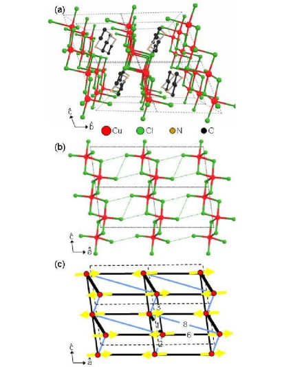
Figure 1: Crystal structure of piperazinium hexachlorodicuprate (PHCC), $\rm(C_{4}H_{12}N_{2})(Cu_{2}Cl_{6})$. (a) View along the a axis, showing well-separated Cu-Cl planes. (b) View of a single Cu-Cl plane. Dotted lines between Cl sites show potential halide-halide contacts. (c) Second view of a single Cu-Cl plane, showing only the interacting Cu²⁺ spin sites (solid circles). Significant antiferromagnetic spin-spin interactions are depicted as light blue (frustrated) and black (satisfied) lines with the same bond numbering used in [24]. Line thickness is proportional to the product of exchange constant and spin-spin correlation function, $|J_{\mathbf{d}}\langle{\mathbf{S}}_{\mathbf{0}}\cdot{\mathbf{S}}_{\mathbf{d}}\rangle|$. Vectors represent the ordered spin structure determined by elastic neutron scattering at $T=1.65$ K and $\mu_{0}H=13.7$ T. Dashed lines are the $\bf{a-c}$ plane unit cell with room temperature lattice constants $a=7.984(4)$ Å, $b=7.054(4)$ Å, $c=6.104(3)$ Å, and $\alpha=111.23(8)^{\circ}$, $\beta=99.95(9)^{\circ}$, and $\gamma=81.26(7)^{\circ}$, space group $P\bar{1}$, from [26].

In the current study, we employed inelastic and elastic neutron scattering as well as specific heat and magnetic susceptibility measurements to characterize the low-temperature phases of PHCC. Unlike 3D coupled-dimer systems, such as $\mathrm{TlCuCl_{3}}$, we find a significant separation between the phase boundary to long range order (LRO) and the crossover line delineating the high-field boundary of the QP regime. This allows access to a disordered renormalized classical (RC-2D) regime near the lower QCP. Specific heat measurements in the disordered low-field QP phase agree well with series expansions from a quantum bilayer model. Combining elastic neutron scattering and field dependent specific heat results allows a determination of the critical exponents associated with the transition to LRO. We have previously reported a reentrant phase transition at low temperature near $H_{c1}$ wherein the magnetic LRO can melt into the QP phase as the temperature is either increased or decreased [27]. We have proposed that coupling between other degrees of freedom is important near the QCP, and thus can have a non-negligible effect on the phase diagram in this regime. We also have recently examined the LRO transition and found good agreement with a representation of the phase boundary away from the reentrant phase transition in terms of magnon Bose-Einstein condensation. In this communication, we provide further experimental and theoretical information regarding these phenomena, including field dependent neutron scattering, magnetization, and specific heat data, and a more detailed theoretical discussion of magnon Bose-Einstein condensation in PHCC.

2 Experimental techniques

Single crystal samples of deuterated and hydrogenous PHCC were prepared via previously described methods [24]. Magnetic susceptibility measurements were performed at the National High Magnetic Field Laboratory pulsed field facility at the Los Alamos National Laboratory using a compensated coil susceptometer. The sample environment consisted of a pumped He³ cryostat located in the bore of a 50 Tesla pulsed field resistive magnet. Measurements were performed with the magnetic field along the b-, a^∗- and c- axes on hydrogenous samples with masses between $m=0.7$ mg and $m=1.4$ mg. An empty coil measurement was performed for each individual pulsed field measurement of the sample as a direct measure of the sample-independent background. Specific heat measurements were performed as a function of magnetic field, $\mu_{0}H\leq 14$ T, and temperature, $T\geq 1.8$ K, on a deuterated single crystal sample, $m=6.76$ mg, with ${\bf H}\parallel$ a^∗ using a commercial calorimeter (Quantum Design PPMS).

Neutron scattering measurements were performed using the FLEX triple axis spectrometer at the cold neutron facility of the Hahn-Meitner Institut in Berlin, Germany. The sample was mounted on an aluminum holder and attached to the cold finger of a dilution refrigerator within a split coil $\mu_{0}H=14.2$ T superconducting magnet. A magnetic field in excess of the superconducting critical field for aluminum was always present to ensure good thermal contact to the sample. The sample consisted of two deuterated single crystals with a total mass of $m=1.75$ g coaligned within 0.5^∘. The sample was oriented in the $(h0l)$ scattering plane with ${\bf H}\parallel$ b. Measurements were performed using a vertically focusing pyrolytic graphite (PG(002)) monochromator followed by a $60^{\prime}$ horizontal collimator. Inelastic measurements used a liquid nitrogen cooled Be filter before the sample and a fixed final energy of $E_{f}=3$ meV. A horizontally focusing PG(002) analyzer was used for inelastic measurements. Elastic measurements employed a flat PG(002) analyzer with $60^{\prime}$ collimation before and after the analyzer. Measurements characterizing the temperature and magnetic field dependence of Bragg peaks used a liquid nitrogen cooled Be filter before the sample and neutron energy $E_{i}=E_{f}=2.5$ meV. Measurements of magnetic and nuclear Bragg peaks for determining the ordered magnetic structure were performed using the same collimation with a room temperature PG filter before the sample and $E_{i}=E_{f}=14.7$ meV with a vertically focusing PG(004) monochromator and a flat PG(002) analyzer.

3 Experimental results

3.1 Susceptibility and magnetization

Pulsed field measurements of the magnetic susceptibility $\chi(H)$ up to $\mu_{0}H=50$ T with ${\bf H}\parallel{\mathbf{b}}$ are shown in figure 2. For $T\leq 4$ K, the susceptibility has two sharp features. The lower field feature marks closure of the spin gap while the upper feature indicates the field where $M(H)$ saturates, and the system enters the fully polarized (FP) regime. $M(H)$ at $T=0.46$ K, obtained by integrating the corresponding $\chi(H)$ data, is shown as a solid line in figure 2. At low temperatures, these features in $\chi(H)$ indicate the location of the critical fields $\mu_{0}H_{c1}\approx 7.5$ T and $\mu_{0}H_{c2}\approx 37$ T. We note that although there is a local minimum in $\chi(H)$ at $\mu_{0}H=23.9$ T near $H_{m}=\frac{1}{2}(H_{c1}+H_{c2})$, and hence a point of inflection in the magnetization, there is no indication of fractional magnetization plateaus for $T\geq 0.46$ K.

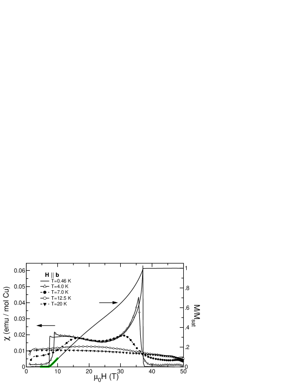
Figure 2: Magnetic susceptibility $\chi$ (left axis) and normalized magnetization $M/M_{sat}$ (right axis) ($T=0.46$ K only) of PHCC vs. magnetic field for ${\bf H}\parallel{\mathbf{b}}$ at different temperatures. Markers are plotted for every thirtieth data point. The green line in the vicinity of $H_{c1}$ is a fit to $M(H)$, as described in the text.

As $T$ increases, the two features in $\chi(H)$ broaden, and above $T=9$ K, they merge into a single rounded maximum that moves to lower fields as the temperature is further increased. For $T>20$ K, $\chi(H)$ decreases monotonically with $H$. Despite the thermal broadening above $T=5$ K, several regimes may be identified from $\chi(H,T)$. These are most clearly seen in figure 3, which shows $\chi(H,T)$ at fixed field. The rounded peak and exponential decrease in $\chi(T)$ for low magnetic fields is characteristic of a gapped antiferromagnet and is similar to prior results obtained at $H=0$ for PHCC [24, 28, 26]. As the field increases, the peak in $\chi(T)$ shifts to lower $T$, and the low-temperature activated behavior vanishes with the spin-gap. As shown for $\mu_{0}H=10$ T in figure 3(a), for fields $\mu_{0}H_{c1}<\mu_{0}H<12$ T the rounded maximum that signals the onset of 2D antiferromagnetic spin correlations leading to the gapped state is still visible (near $T=12$ K for $\mu_{0}H=10$ T), but there is then a sharp rise in $\chi(T)$ as the system enters the strongly magnetizable regime at lower $T$. As shown in figures 3(a) and 3(b) the boundary of this regime continues to move to higher $T$ for $\mu_{0}H<$ 25 T, before moving back to lower $T$ as $H$ approaches $H_{c2}$. In the FP region above $H_{c2}$ activated behavior returns, as shown for $\mu_{0}H=40$ T and $\mu_{0}H=47$ T in figure 3(c). This indicates a second spin-gap regime. Note that as the field increases above $H_{c2}$, the onset of the activated susceptibility moves to higher $T$, indicating that this second spin gap increases with field. An overview of $\chi(H,T)$ is given in the color contour plot in figure 11(a) and will be discussed in more detail below.

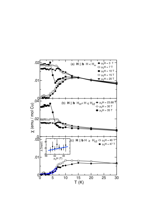
Figure 3: Magnetic susceptibility of PHCC as a function of temperature for ${\bf H}\parallel{\mathbf{b}}$. (a) $\mu_{0}H\leq 20$ T, (b) 23 T $\leq\mu_{0}H<\mu_{0}H_{c2}$, (c) $H>H_{c2}$. Data were obtained by combining all individual pulsed field measurements and averaging over the range $\mu_{0}(\Delta H)=0.5$ T for each magnetic field shown. Lines connecting data points are guides to the eye. Curves in (c) for $T<8$ K are fits described in the text that yield the field dependence of the gap above $H_{c2}$ shown in the inset to (c). The solid line in the inset to (c) has the slope $g\mu_{B}H$.

Low-temperature pulsed field susceptibility measurements were also performed at $T=0.46$ K for ${\bf H}\parallel\mathbf{c}$ and ${\bf H}\parallel\mathbf{a^{*}}$. These are shown together with the ${\bf H}\parallel\mathbf{b}$ data near $H_{c1}$ and $H_{c2}$ in figure 4. Although the overall shape of $\chi(H)$ is similar in all three orientations, the differences in the onset fields shown in figure 4 indicate that the critical fields are orientation-dependent. Because the ratio of the critical fields is nearly the same for each of the three single crystal orientations, [$H_{c1}({\mathbf{b}})/H_{c2}({\mathbf{b}})=$ 0.203(3), $H_{c1}({\mathbf{c}})/H_{c2}({\mathbf{c}})=$ 0.203(3), and $H_{c1}({\mathbf{a}}^{*})/H_{c2}({\mathbf{a}}^{*})=$ 0.205(3)], differences in the magnitude of the critical fields are likely due to $g$-factor anisotropy associated with the coordination of the Cu²⁺ ions in PHCC.

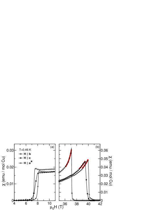
Figure 4: Magnetic susceptibility of PHCC at $T=0.46$ K for ${\bf H}\parallel{\mathbf{b}}$, ${\bf H}\parallel{\mathbf{c}}$, and ${\bf H}\parallel{\mathbf{a}^{*}}$ in the vicinity of (a) $H_{c1}$ and (b) $H_{c2}$. Data obtained for different sample masses were normalized to the saturation magnetization for ${\bf H}\parallel{\mathbf{b}}$. Solid red lines are fits in the vicinity of the upper critical fields as described in the text. Markers are plotted every seventh datapoint.

3.2 Specific heat

Measurements of the specific heat as a function of temperature and magnetic field are shown in figure 5. Prior measurements were performed on protonated samples in the same orientation, ${\bf H}\parallel{\mathbf{a}}^{*}$, but were restricted to $T\leq 2$ K and $\mu_{0}H\leq 9$ T. The total specific heat $C_{p}$ is shown for representative fields in figure 5(a). In zero field, $C_{p}$ shows a broad rounded maximum at $T\approx 7$ K, with an exponentially activated region at lower $T$ associated with the formation of the spin-gap. Above $H_{c1}$ the form of the high-temperature specific heat changes, and as shown for $\mu_{0}H=14$ T, a lambda-type anomaly can be seen that is associated with the phase transition to magnetic LRO at $T=T_{N}$. In figure 5(b) we plot the magnetic portion of the specific heat, $C_{m}=C_{p}-C_{\mathrm{lattice}}$, where $C_{\mathrm{lattice}}\propto T^{3}$ is the lattice/phonon contribution to the specific heat determined by comparison of the data to the bilayer model discussed later in the text. This lattice contribution is shown as a dashed line in figure 5(a). Figure 5(b) shows the changes in the low-field activated behavior of $C_{m}$ as $H$ increases and the spin-gap closes, as well as the increase in magnitude of the lambda peaks as $H$ increases above $H_{N}$. The area under the peak is greater for larger applied fields indicating that the $T=0$ ordered moment increases with magnetic field. The field dependence of $C_{p}$ is plotted in figure 5(c) for selected temperatures. We observe a sharp peak at the transition to LRO at $H=H_{N}$, which has the same field and temperature dependence as that seen in $C_{p}(T)$ at fixed $H$.

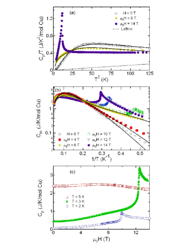
Figure 5: Specific heat as a function of temperature and magnetic field for deuterated PHCC with ${\bf H}\parallel{\mathbf{a}}^{*}$. (a) Total specific heat $C_{p}/T$ vs. $T^{2}$ at fixed $H$. Every tenth data point is plotted for $\mu_{0}H=14$ T. Calculated lattice contribution is shown as a dashed line. (b) Magnetic specific heat $C_{m}=C_{p}-C_{\mathrm{lattice}}$ vs. $1/T$. Solid lines for $\mu_{0}H<10$ T in (a) and (b) are the result of a global fit to the frustrated bilayer model discussed in the text. (c) Isothermal specific heat.

3.3 Elastic neutron scattering

Neutron diffraction was used to explore the nature of the LRO transition indicated by heat capacity data. Field and temperature dependent antiferromagnetic Bragg peaks were observed at wave vector transfer ${\bf Q}=(\frac{(2n+1)}{2}$, $0$, $\frac{(2m+1)}{2})$ for integer $n$ and $m$ throughout the $(h0l)$ plane, corresponding to a magnetic structure with a doubling of the unit cell along the a- and c-axes.

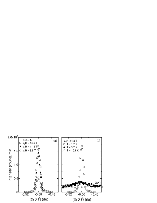
Figure 6: Wave-vector dependent elastic scattering from PHCC as measured through the $(\frac{1}{2}0\bar{\frac{1}{2}})$ Bragg peak along the $(\frac{1}{2}0l)$ direction. (a) Magnetic field, ${\bf H}\parallel{\mathbf{b}}$, dependence at $T=1.7$ K. (b) Temperature dependence at $\mu_{0}H=14.2$ T.

Figure 6 depicts a wave-vector scan through the $(\frac{1}{2}0\bar{\frac{1}{2}})$ Bragg peak as a function of (a) magnetic field and (b) temperature. The scattering intensity at $T=1.7$ K increases as a function of applied field. At $\mu_{0}H=14.2$ T (figure 6(b)) there is only a flat background at $T=10.1$ K; however, for $T=3.7$ K the broad maximum indicates short range AFM correlations. At $T=1.7$ K the resolution limited peak indicates long range antiferromagnetic order. Scans along the $(h0\bar{\frac{1}{2}})$ and $(\zeta 0\bar{\zeta})$ directions were also resolution limited. Magnetic Bragg peaks were found at locations that were indistinguishable from the nuclear half-wavelength, $\lambda/2$, Bragg peaks, which were observed upon removal of the Be filter to admit $\lambda/2$ neutrons from the PG(004) monochromator Bragg reflection. No indication of incommensurate order was found along the $(h0\bar{\frac{1}{2}})$ and $(\frac{1}{2}0l)$ directions through the entire Brillouin zone at $T=1.9$ K and $\mu_{0}H=11.8$ T.

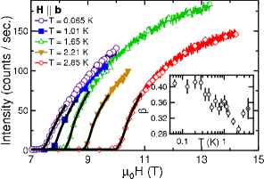
Figure 7: Magnetic field, ${\bf H}\parallel{\mathbf{b}}$, dependence of elastic scattering intensity of the $(\frac{1}{2}0\bar{\frac{1}{2}})$ Bragg peak at select temperatures. Temperatures presented increase according to the figure legend from left to right. Solid lines are fits described in the text over the region $\mu_{0}H<\mu_{0}H_{N}+0.75$ T. Inset: magnetic order parameter critical exponent, $\beta$, determined by fitting a power law $I(H)\propto(H-H_{N})^{2\beta}$ to magnetic field and temperature dependent scattering from the $(\frac{1}{2}0\bar{\frac{1}{2}})$ antiferromagnetic Bragg peak. The Data point at $T=3.69$ K corresponds to the temperature scan shown in figure 8.

To characterize the onset of antiferromagnetic order, the $(\frac{1}{2}0\bar{\frac{1}{2}})$ Bragg peak was measured as a function of magnetic field at sixteen temperatures for $0.065\leq T\leq 2.85$ K. Data were obtained by continuously sweeping the magnetic field ($\mu_{0}dH/dt=0.01$ or $0.03$ T/min.) while simultaneously counting diffracted neutrons over a fixed time interval of 0.5 minutes per point. At T=0.06 K the measured field trace was indistinguishable for the slower and faster rates. The results are shown for select temperatures in figure 7. The temperature dependence of the $(\frac{1}{2}0\bar{\frac{1}{2}})$ Bragg peak at $\mu_{0}H=14.2$ T was measured by integrating over a series of rocking curves at 37 temperatures as shown in figure 8. The intensity increases continuously upon cooling below a distinct critical temperature as expected for a second order phase transition.

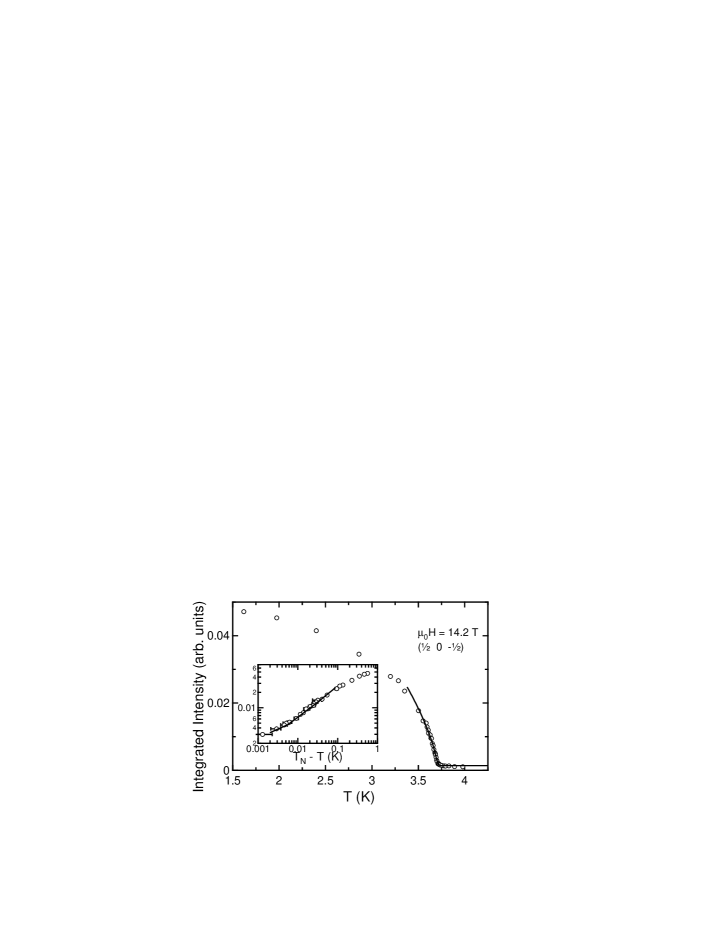
Figure 8: Temperature dependence of $(\frac{1}{2}0\bar{\frac{1}{2}})$ antiferromagnetic Bragg peak elastic scattering intensity for PHCC at $\mu_{0}H=14.2$ T with ${\bf H}\parallel{\mathbf{b}}$. Data points were obtained from the integrated intensities of rocking curves measured at each temperature. Inset: Log-Log plot of integrated intensity as a function of the difference between the determined Néel temperature, $T_{N}=3.705(3)$ K, and the sample temperature. Solid lines are fits as described in text over the range $T>T_{N}-0.33$ K.

Figures 9(a) and  9(c) show low-temperature magnetic field sweeps of the $(\frac{1}{2}0\bar{\frac{1}{2}})$ magnetic Bragg intensity plotted as a contour plot and as intensity versus field in the vicinity of the critical field for the transition to Néel order, which we denote by $H_{N}$. The data indicate that the ordered phase is thermally reentrant for $\mu_{0}H\approx 7.5$ Tesla. Upon heating from 0.065 K, $H_{N}$ initially decreases with increasing temperature. However, there is an apparent minimum in the critical field curve at $T=0.20$ K, above which temperature $H_{N}$ increases on heating. The same data are plotted as a function of temperature at fixed fields in figure 9(b). These data show a peak in the scattering intensity at $T=0.20$ K for fields between $\mu_{0}H\approx 7.45$ T and $\mu_{0}H\approx 7.9$ T. The peak location remains at $T\approx 0.2$ K until vanishing for fields above $\mu_{0}H\approx 8.1$ T.

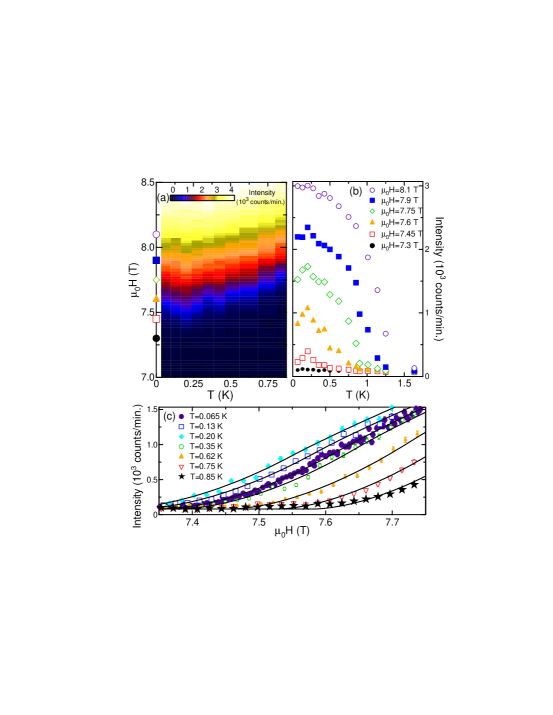
Figure 9: Reentrant behavior of low-temperature LRO phase as a function of magnetic field, ${\bf H}\parallel{\mathbf{b}}$, and temperature. (a) Elastic scattering intensity of the $(\frac{1}{2}0\bar{\frac{1}{2}})$ antiferromagnetic Bragg peak as a function of applied magnetic field and temperature. False color image obtained by combining all individual magnetic field order parameter scans. (b) Elastic scattering intensity of the $(\frac{1}{2}0\bar{\frac{1}{2}})$ antiferromagnetic Bragg peak as a function of temperature. Data were obtained by combining all of the individual magnetic field order parameter scans and averaging over $\mu_{0}\Delta H=0.1$ T for each magnetic field shown. The symbols on the vertical axis in (a) correspond to constant temperature data shown in (b). (c) Magnetic field order parameter scans of the $(\frac{1}{2}0\bar{\frac{1}{2}})$ antiferromagnetic Bragg peak performed in the region of the reentrant phase transition. Solid lines are fits described in the text.

3.4 Inelastic neutron scattering

Inelastic neutron scattering was used to probe spin-dynamics as a function of magnetic field and temperature. In particular, constant wave vector scans at ${\bf Q}=(\frac{1}{2}0\bar{\frac{1}{2}})$ were performed as a function of magnetic field at $T=0.06$ K and $T=4.5$ K. A portion of these data is shown in figure 10. The low-temperature scan at $H=0$ T features a resolution limited excitation at $\hbar\omega\approx 1$ meV, consistent with the previous zero field measurements [24]. In an applied field this excitation splits into three components indicating a zero field triplet 1 meV above a singlet ground state. The intensity distribution is consistent with the upper and lower peaks resulting from transitions to $S_{z}=\pm 1$ states while the central highest intensity peak corresponds to a transition to an $S_{z}=0$ state. The lower energy, $S_{z}=+1$, peak is observable until $\mu_{0}H\approx 6$ T, where it is obscured by elastic nuclear incoherent scattering. Both remaining gapped excitations increase in energy continuously as the field is increased above $H_{c1}$. The higher energy excitation increases in energy and decreases in intensity at a faster rate than the excitation which evolves out of the $S_{z}=0$ component of the $H<H_{c1}$ triplet. There are also subtle differences in the temperature and field dependence of the width of the excitations, which we shall return to later.

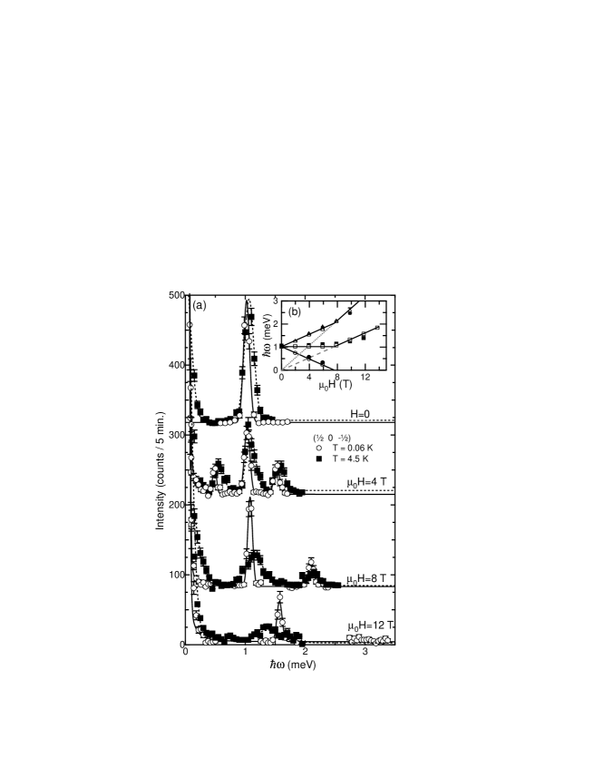
Figure 10: (a) Constant wave-vector $(\frac{1}{2}0\bar{\frac{1}{2}})$ inelastic neutron scattering from PHCC at $T=0.06$ K (open symbols) and $T=4.5$ K (solid symbols) for different values of applied magnetic field, ${\bf H}\parallel{\mathbf{b}}$. Solid(dashed) lines are fits to Gaussians for the low(high) temperature data as described in the text. Data are offset vertically for clarity. (b) Peak locations derived from data such as that shown in (a) as a function of applied magnetic field. Solid lines are a fit to the $T=0.06$ K data as described in text. Dashed lines extend these lines to the origin.

4 Discussion

4.1 Susceptibility and magnetization

A second view of the magnetic susceptibility data shown in figures 2 and 3 is provided by the color contour map in figure 11(a). Since the sharp features in $\chi(H)$ at the lowest-$T$ herald the onset of finite magnetization at $H_{c1}$ and the entry into the fully polarized (FP) regime at $H_{c2}$, we identify the continuation of these features for $T\leq 5$ K as experimental signatures of the closing of the low-field spin gap and the opening of the high-field spin gap with increasing field in the vicinity of the critical fields $H_{c1}$ and $H_{c2}$, respectively. These features provide a starting point in constructing an $H$-$T$ phase diagram for PHCC, and are shown as open circles in figure 11(b). By extending these points through inclusion of the sharp features visible in $\chi(T)$ for $T>5$ K, they are seen to demarcate the entire large-susceptibility region in figure 11(a). At non-zero $T$, these points delineate a crossover, rather than a phase transition. Near the lower QCP $H_{c1}$, for example, this boundary marks the change from the non-magnetized quantum paramagnet (spin-gap) regime to a quasi-2D renormalized classical (RC-2D) region with finite magnetization.

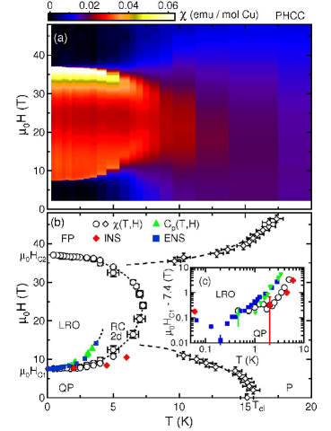
Figure 11: (a) Color contour map of $\chi(H,T)$ for PHCC. (b) Magnetic field versus temperature phase diagram of PHCC. $H_{c1}$ and $H_{c2}$ are zero-temperature QCPs described in the text. Data points were obtained from pulsed field susceptibility ($\chi(T,H)$), inelastic neutron scattering (INS), elastic neutron scattering (ENS), and specific heat measurements ($C_{P}(T,H)$). Specific heat measurements were performed with ${\bf H}\parallel{\mathbf{a}}^{*}$; all other measurements were made with ${\bf H}\parallel{\mathbf{b}}$. Values from $C_{P}(T,H)$ have been renormalized as discussed in the text. LRO indicates a long range ordered phase; QP is a quasi-2D quantum paramagnetic phase; FP corresponds to a ferromagnetic polarized phase; RC-2D indicates a quasi-2D renormalized classical phase; and P corresponds to the semi-classical paramagnetic region. Dashed lines are guides to the eye. Open diamonds represent the rounded peak locations in $\chi(T)$ delineating a higher temperature classical paramagnetic regime from the correlated low-temperature regimes, QP and FP. Open circles represent locations of sharp features in $\chi(T)$ and $\chi(H)$. Closed diamonds correspond to the closing of the spin-gap as determined from INS data in figure 15. Closed squares represent transitions to long range order as determined from the field and temperature dependence of the $(\frac{1}{2}0\bar{\frac{1}{2}})$ antiferromagnetic Bragg peak shown in figures 7 and  8. (c) Log-log plot of the low-temperature reentrant behavior of the LRO phase.

We also identify two additional crossovers in the $H$-$T$ plane of PHCC that are defined by rounded maxima in $\chi(T)$ for $H<H_{c1}$ and $H>H_{c2}$. These are demarcated by open diamonds in figure 11(b). At low field, the resulting boundary indicates where antiferromagnetic correlations begin to develop as the system is cooled toward the spin gap regime. This process has been well-studied in other spin gap systems, such as Haldane spin-1 chains [29]. The intersection of this crossover with the zero-field axis in figure 11(b) marks the onset of a high-temperature semi-classical paramagnetic regime (P) where the system has not yet attained significant antiferromagnetic correlations and the magnetic susceptibility is that of a disordered ensemble of exchange-coupled spins with one energy scale, i.e. Curie-Weiss behavior.

The high field crossover regime (open diamonds above $H=H_{c2}$ in figure 11(b)) is not as well characterized experimentally, but should mark the onset of appreciable ferromagnetic correlations as the system is cooled at high field toward the FP state. The excitations in the FP state are expected to be ferromagnetic spin waves. As for a conventional ferromagnet in a field, these excitations will show a field-dependent gap, although here the energy scale for the gap should be set by $\Delta_{FP}=g\mu_{B}(H-H_{c2})$. Fits of the form $\chi(T)\propto e^{-\Delta/k_{B}T}$, such as those shown in figure 3(c), yield estimates for the gap in the FP regime. Values of $\Delta_{FP}$ as determined from a simultaneous fit of $\chi(T)$ in the temperature range $0.75\leq T\leq 6$ K for $40\leq\mu_{0}H\leq 47$ T are shown in the inset of figure 3(c) and are consistent with a linear increase of $\Delta_{FP}$ with field above $H_{c2}$.

The evolution of the magnetic susceptibility as a function of magnetic field and temperature has been examined numerically for the two-leg spin-ladder [30]. Calculations depict a low-temperature field dependent magnetization, which is symmetric about $H_{m}=\frac{1}{2}(H_{c1}+H_{c2})$ with square root singularities near the upper and lower critical fields, consistent with results for other 1D spin-gap systems [31]. Its phase diagram is thus similar to our findings for PHCC. The calculations also report similar susceptibility anomalies: a double peaked function at low temperatures, a single rounded peak that moves to lower fields as the temperature is increased, and a monotonically decreasing field dependence as the temperature is increased beyond a certain temperature, $T_{{\mathrm{c}l}}$. A crossover temperature marking the boundary between the classical and quantum regimes, was identified as $T_{{\mathrm{c}l}}=1.109\Delta/k_{B}$ for the two-leg spin ladder. For PHCC, this corresponds to $T_{{\mathrm{c}l}}=1.109\Delta/k_{B}=13.1$ K which agrees well with the zero-field lower temperature bound of the crossover regime defined in figure 11 where we find $T_{{\mathrm{c}l}}\approx 15.4$ K based upon susceptibility measurements.

Close to the critical fields the low-temperature field dependent magnetization should follow power laws of the form $M\propto|H-H_{c}|^{1/\delta}$, where $H_{c}$ is a critical field [32]. In terms of magnetic susceptibility, this power law becomes

$$\chi_{+}=dM/dH\propto(H-H_{c1})^{1/\delta_{1}-1}$$ (2a)

$$\chi_{-}=dM/dH\propto(H_{c2}-H)^{1/\delta_{2}-1}$$ (2b)

immediately above ($\chi_{+}$) and below ($\chi_{-}$) the respective lower and upper critical fields. For PHCC Figures 2 and 4 indicate that $\delta_{2}>\delta_{1}\approx 1$ to account for the observed curvature near the critical fields. Because $\delta_{1}\approx 1$, we fit $M(H)$ rather than $\chi(H)$ to determine $\delta$. This is done simultaneously for all $T=0.46$ K single crystal orientations with a common value of $\delta_{1}$ over a range of one Tesla above $H_{c1}$. The single crystal low-temperature, $T=0.46$ K data were also simultaneously fit over a range of one Tesla below $H_{c2}$ using Eqn. (2b). The simultaneous fits shared a common $\delta$ parameter; whereas critical fields and overall amplitudes were allowed to vary between the different orientations. The resulting values, $\delta_{1}=0.91(1)$ and $\delta_{2}=1.8(2)$, and their corresponding power-laws are shown in figures 2 and 4. For comparison, 1D singlet ground state systems are predicted to have symmetric susceptibility and magnetization curves with $\delta_{1}=\delta_{2}=2$ [32], and the 2D square lattice Heisenberg model has an analogous upper critical field with predictions ranging from $\delta_{2}=1$ to $\delta_{2}=1$ with logarithmic corrections [33, 34]. An interpretation of $H_{c1}$ as magnon Bose-Einstein condensation yields the prediction of $\delta_{1}=1$ (see section 4.5).

4.2 Specific heat

We compare our specific heat measurements to the frustrated bilayer model of Gu and Shen [35]. Their model contains a strong interlayer bond $J_{0}$, a weaker intralayer bond $J_{1}$, and a frustrating interlayer bond $J_{2}$. This exchange topology is similar to that in PHCC. We include a magnetic field dependent term in their thermodynamic expansion via a linear Zeeman splitting of the triplet excited state as a function of applied magnetic field. We carried out a global fit of all our specific heat data with $\mu_{0}H\leq 9$ T and $T\leq 30$ K using only the free energy terms up to powers of $1/E^{-2}$ in Gu and Shen’s expansion, one independent prefactor for each magnetic field, and global terms consisting of the three exchange constants, a $g$-factor and a lattice contribution $\propto T^{3}$. The results of this fit are shown as solid lines in figure 5 and account very well for the temperature and field dependence with $J_{0}=2.08(1)$ meV, $J_{1}=0.34(3)$ meV and $J_{2}=-0.13(3)$ meV

The exchange parameters for the frustrated bilayer model determined from the specific heat data for PHCC can be used to evaluate the corresponding dispersion relation, equation 4 of Ref. [35]. Figure 12 depicts the calculated dispersion for PHCC along several high-symmetry directions in reciprocal space, compared to the zero-field triplon dispersion measured by inelastic neutron scattering [24, 25]. The values derived from the fits to $C_{m}$ for the spin gap $\Delta=1.11(1)$ meV and bandwidth of 1.92(2) meV agree quite well with the measured spin gap, $\Delta=0.99$ meV and bandwidth, 1.73 meV. Furthermore, the frustrated bilayer model reproduces the shape of the dispersion remarkably well given that specific heat data provided the only experimental input.

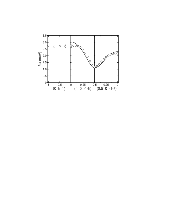
Figure 12: Zero-field magnon (or triplon) dispersion in PHCC. Data taken from Refs [24] and [25]. Solid lines are the calculated dispersion based upon fitting magnetic heat capacity to the bilayer model as described in the text.

The lambda-type peaks in the magnetic heat capacity yield an additional measure of the boundary on the magnetic field vs. temperature phase diagram for PHCC, figure 11(b), between the quasi-2D RC-2D disordered phase and the LRO phase. However, $C_{p}$ was measured with ${\bf H}\parallel{\mathbf{a}}^{*}$, while all the other data included in figure 11(b) were measured with ${\bf H}\parallel{\mathbf{b}}$. As noted above, differences in the critical fields measured for $\chi(H)$ for different field orientations are accounted for by g-factor anisotropy. After rescaling by the ratio $H_{c1}({\bf H}\parallel{\mathbf{b}})/H_{c1}({\bf H}\parallel{\mathbf{a}}^{*})=0.917$ determined from $\chi(H)$, the phase boundary derived from $C_{p}(H,T)$ is seen to agree very well with that determined from elastic neutron scattering as shown in figure 11(b) and (c) and discussed below.

The magnetic field dependent specific heat shown in figure 5(c) also provides a sensitive measure of critical scaling in the vicinity of the LRO transition. $C_{m}(H)$ is shown in figure 13 as a function of reduced magnetic field, $h=|\frac{H-H_{N}}{H_{N}}|$ near the transition field $H_{N}$. Power law behavior is clearly seen for $H>H_{N}$, while below $H_{N}$, the magnetic specific heat asymptotically approaches the same power law behavior as the $H>H_{N}$ portion of the data. In addition, there is a region of reduced field for $H<H_{N}$, $0.02\leq h\leq 0.2$, where we observe a different power-law behavior, i.e. a different slope on the log-log scale plot as indicated by the dashed line in figure 13. The two different power-laws observed for $H<H_{N}$, as shown by the fits for $0.02\leq h\leq 0.2$ and the asymptotic change in power-law as one approaches $H_{N}$ is a potential indication of an additional disordered portion of the phase diagram for $H<H_{N}$. This is in fact directly measured as a gapless disordered region through comparisons of the magnetic susceptibility and neutron scattering measurements as we discuss later in the text and as shown in figures 11(b) and (c).

We fit the $H>H_{N}$ data in figure 13 to a power law of the form

$$C_{m}=A(h)^{-\alpha},$$ (2c)

where $\alpha$ is the specific heat exponent. A global fit for $T=2$ K and $3$ K results in $\alpha=0.097(2)$ while individual fits yield $\alpha(T=2\mathrm{K})=0.104(3)$ and $\alpha(T=3\mathrm{K})=0.072(2)$. Individual fits to Eq. 2c for $H<H_{N}$ over the range $0.02\leq h\leq 0.2$ yield $\alpha(T=2\mathrm{K})=0.175(2)$ and $\alpha(T=3\mathrm{K})=0.2626(7)$. These values are larger than those obtained for $H>H_{N}$, which indicates that the fits include data beyond the critical regime. Table 1 summarizes theoretical and experimental results for the 3D magnets.

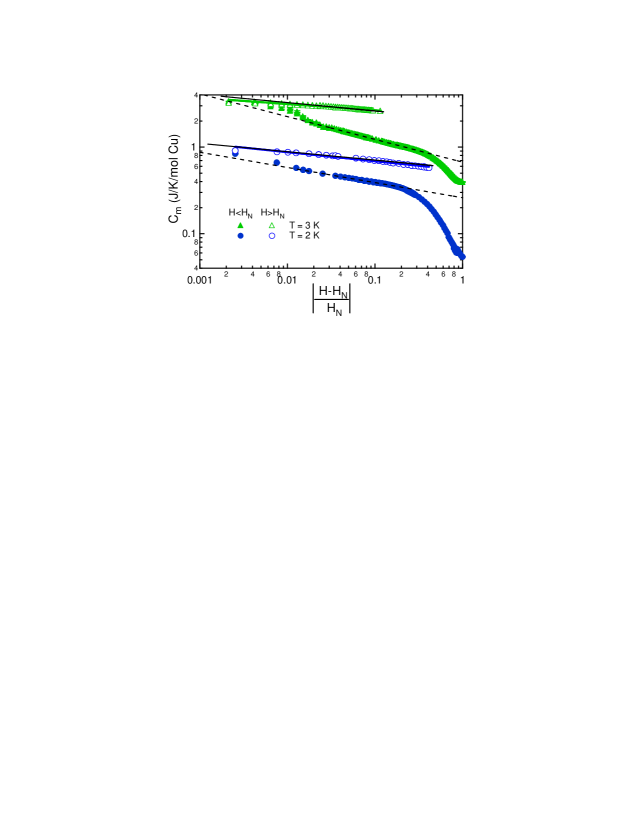
Figure 13: Magnetic heat capacity as a function of reduced magnetic field, $h$, in the vicinity of the phase transition to LRO. $H<H_{N}$ data (solid symbols) are plotted against $h=\frac{H_{N}-H}{H_{N}}$. $H>H_{N}$ data (open symbols) are plotted against $h=\frac{H-H_{N}}{H_{N}}$. Black solid lines correspond to a global fit of $H>H_{N}$ data to a power law as discussed in text. Coloured solid lines correspond to individual power law fits for $H>H_{N}$. Individual fit results are very similar to the global fit result. Dashed lines correspond to individual power law fits for $H<H_{N}$ for $0.025\leq h\leq 0.2$ in the RC-2D regime.

Table 1: Measured exponents for PHCC compared to calculated exponents listed in [36, 37, 38, 39] for both 3D Heisenberg (HB), XY (3D), and Ising (2D and 3D) transitions. Errors in referenced values are listed when available. Error bars for $\alpha$ in PHCC correspond to one standard deviation greater and less than the respective maximum and minimum fitted values described in the text.

		Calc. HB	Calc. XY	2D Ising	Calc. 3D Ising
	PHCC	Ref [37]	Ref [38]	Ref [36]	Ref [39]
$\alpha$	$0.097^{+0.010}_{-0.027}$	-0.1336(15)	-0.0146(8)	0	0.1099(7)
$\beta$	0.34(2)	0.3689(3)∗	0.3485(2)∗	0.125	0.32648(18)∗
$\gamma$	1.22(4)∗	1.3960(9)	1.3177(5)	1.75	1.2372(4)
$\delta$	4.6(2)∗	4.783(3)∗	4.780(2)∗	15	4.7893(22)∗
$\nu$	0.634(1)∗	0.7112(5)	0.67155(27)	1	0.63002(23)
$\eta$	0.07(6)∗	0.0375(5)	0.0380(4)	0.25	0.0364(4)

^∗Calculated from scaling relations and other listed critical exponents. Error bars propagated from the measurements or calculations via the scaling laws.

4.3 Elastic neutron scattering

4.3.1 Ordered magnetic structure

To determine the field induced magnetic structure we measured fourteen magnetic Bragg peaks in the $(h0l)$ plane. The measurements were carried out at $T=1.65$ K and $\mu_{0}H=13.7$ T which is within the ordered phase as established by heat capacity measurements. Table 2 shows raw experimental results in the form of wave vector integrated intensities, $I_{m}(\tau_{m})$, for transverse (rocking) scans. $I_{m}(\tau_{m})$ is related to the magnetic structure of the material as follows:

$$I_{m}(\tau_{m})={\cal C}\int{\cal R}_{\tau}({\bf q}_{\perp})d{\bf q}_{\perp}N_{m}\frac{(2\pi)^{3}}{v_{m}}{\cal I}_{m}(\tau_{m}).$$ (2d)

Here $\cal C$ is a normalization factor that depends on aspects of the instrument such as the incident beam flux that are not considered in the elastic resolution function ${\cal R}_{\tau}({\bf q})$[40] which is sharply peaked around ${\bf q}=0$. $N_{m}$ and $v_{m}$ are the number of magnetic unit cells and the magnetic unit cell volume respectively. The magnetic Bragg scattering intensity is given by

$${\cal I}_{m}({\bf Q})=r_{0}^{2}(|{\bf\cal F}({\bf Q})|^{2}-|\hat{\bf Q}\cdot{\cal F}({\bf Q})|^{2}),$$ (2e)

where $r_{0}=5.38$ fm,[41]

$${\bf\cal F}({\bf Q})=\sum_{\bf d}\frac{g_{\bf d}}{2}F_{\bf d}({\bf Q}))e^{-W_{\bf d}({\bf Q})}{\bf S}_{\bf d}$$ (2f)

is the magnetic structure factor, $g_{\bf d}$ is the Lande g-factor for the magnetic ion on site $\bf d$ within the magnetic unit cell, and $F_{\bf d}({\bf Q})$ is the magnetic form factor of the Cu²⁺ ion [42, 41]. The magnetic structure enters through the expectation values for the spin vector, ${\bf S}_{\bf d}$ in units of $\hbar$.

Table 2 compares the measured scattering intensity $I_{m}(\tau_{m})$ to the calculated intensity for the uniaxial magnetic structure that best fits the data and is shown in figure 1. The ordered moment lies within $\sim 7(4)^{\circ}$ of the a-c-plane and the in-plane component is within $\sim 6(4)^{\circ}$ of the a-axis. For $T=1.65$ K and $\mu_{0}H=13.7$ T the sub-lattice magnetization is $g\mu_{B}\langle S\rangle=0.33(3)g\mu_{B}$, determined by normalization to incoherent scattering of the sample. Assuming antiferromagnetic interactions, the ordered structure is consistent with the sign of the bond energies determined on the basis of zero-field inelastic neutron scattering.[24]

Table 2: Measured and calculated relative magnetic Bragg peak scattering intensities at the indicated magnetic reciprocal lattice points $\tau_{m}=h{\bf a}^{*}+l{\bf c}^{*}$. The parentheses indicate statistical errors only. The minimum in the crystallographic reliability index $R=\sum|I_{m}^{obs}-I_{m}^{calc}|/\sum I_{m}^{obs}=0.3$ is found for the magnetic structure depicted in figure 1 and described in the text.

• $h$	$l$	$I_{m}$ (obs)	$I_{m}$ (calc)
  1	-1/2	0.00(1)	0
  1	1/2	0.00(1)	0
  -1	-1/2	0.00(1)	0
  1/2	-1	0.00(1)	0
  -1/2	-1	0.00(1)	0
  3/2	1/2	0.01(1)	0.002
  1/2	-1/2	1.00(2)	1
  -1/2	-1/2	0.21(1)	0.234
  3/2	-1/2	0.16(1)	0.333
  1/2	-3/2	0.11(1)	0.250
  5/2	1/2	0.03(1)	0.027
  7/2	5/2	0.04(2)	0.154

4.3.2 Phase diagram

Figures 7, 8 and 9(c) compare the temperature and field dependence of the magnetic Bragg intensity at $Q=(\frac{1}{2}0\bar{\frac{1}{2}})$ to power laws $I(H)\propto(H-H_{N})^{2\beta}$ and $I(T)\propto(T_{N}-T)^{2\beta}$ in order to extract the critical exponent, $\beta$. Rounding in the vicinity of the phase transition was accounted for as a distribution in the critical field. Possible origins of the 3.6% distribution width include inhomogeneities in the applied field and chemical impurities. Least squares fitting included only data within 0.75 T and 0.33 K of criticality. The corresponding fits appear as solid lines in the figures.

Values of $(T_{N},H_{N})$ extracted from the analysis appear as filled squares on Figure 11. There is a clear distinction between the onset of a state of high differential susceptibility as determined from $\chi(H,T)$ and the boundaries of the long range ordered phase (LRO) extracted from neutron diffraction data. We denote the state of the system between these boundaries as 2D renormalized classical. Spin correlations in this phase were examined by quasi-elastic neutron scattering measurements along the $(\frac{1}{2}0l)$ and $(h0\bar{\frac{1}{2}})$ directions through the $(\frac{1}{2}0\bar{\frac{1}{2}})$ wave-vector at $T=3$ K and $\mu_{0}H=9$ T. No magnetic Bragg peaks were encountered. Instead the broad peak centered at ${\bf Q}=(\frac{1}{2}0\bar{\frac{1}{2}})$ indicates short range correlations with the same local structure as the long range order that sets in at slightly higher fields.

4.3.3 Critical exponents

The order parameter critical exponent, $\beta$, determined for each of the fits to the magnetic field and temperature dependent scans is shown versus temperature in the inset to figure 7. For $T\geq 0.5$ K, the average value is $\beta=0.34(2)$ which is indistinguishable from the critical exponent for the 3D Heisenberg [37], Ising ($\beta=0.326$), and XY ($\beta=0.345$) models[36]. However, the positive specific heat critical exponent, $\alpha$, uniquely identifies the phase transition as being in the 3D Ising universality class. This is consistent with expectations for a phase transition to long range magnetic order in space group $P\bar{1}$. We also calculate the remaining critical exponents based upon the Rushbrooke , $\alpha+2\beta+\gamma=2$, Fisher, $\gamma=\nu(2-\eta)$, Josephson, $2-\alpha=\nu d$, and Widom, $\delta=1+\frac{\gamma}{\beta}$, scaling laws, assuming $d=3$ dimensions [36, 43]. The values are again consistent only with those of 3D Ising transitions as summarized in  table 1. Recalling the exponents $\delta_{1}=1.022(2)$ and $\delta_{2}=1.8(1)$ in  (2a) and  (2b) determined from pulsed field magnetic susceptibility data, note that these values are different from $\delta$ derived from the scaling relations. This is because $\delta_{1}$ and $\delta_{2}$ are associated with the uniform susceptibility while $\delta$ in table table 1 characterizes the response to a staggered field conjugate to the Néel order parameter.

The apparent order parameter critical exponent increases as temperature is reduced, such that $\beta=0.40(1)$ for $T\leq 0.43$ K (see inset to figure 7). A possible interpretation of this behavior is that the system enters a crossover regime associated with the approach to quantum criticality. Indeed, in the $T=0$ limit the system should be above its upper critical dimension such that mean field behavior with a critical exponent $\beta_{mf}=0.5$ should be expected.

The field sweeps of the ${\bf Q}=(\frac{1}{2}0\bar{\frac{1}{2}})$ magnetic Bragg peak intensity shown in figure 9(a)-(c), indicate a reentrant phase transition. The $H-T$ phase boundary obtained by fitting these data (figure 11(b)) show a local minimum in the phase boundary between the LRO and QP phases. A possible origin of this anomaly is coupling to non-magnetic degrees of freedom such as nuclear spin or lattice distortions that are unimportant at higher temperatures but become important sufficiently close to the quantum critical point[27].

4.4 Inelastic neutron scattering

4.4.1 Gapped Excitations

Figure 10 shows the magnetic field and temperature dependence of the excitation spectrum at the critical wave vector ${\bf Q}=(\frac{1}{2}0\bar{\frac{1}{2}})$ for $0\leq H<H_{c2}$. We fit each spectrum to a sum of Gaussian peaks to account for the magnetic excitations with a constant background and a field independent Gaussian+Lorentzian lineshape centered at zero energy to account for incoherent elastic nuclear scattering. The field dependence of the peak locations are plotted for the $T=0.06$ K and $T=4.5$ K data in figure 10(b). The data demonstrate the triplet nature of the excited state through its Zeeman splitting. Above $H_{c1}$, the rate of change of the peak position as a function of field for the higher energy peak is twice that of the lower energy excitation, indicating a magnetized ground state. We fit the low $T$ field dependent peak locations to the spectrum of an antiferromagnetically coupled spin-1/2 pair with singlet-triplet splitting $\Delta$ subject to a magnetic field described by ${\cal H}_{Z}=-g\mu_{B}\mu_{0}H$. Results of this two-parameter fit to the low-temperature peak locations are plotted as solid lines in figure 10(b), and yield values of $\Delta=1.021(2)$ meV, $g=2.33(1)$, and $\mu_{0}H_{c1}=\Delta/(g\mu_{B})=7.58(3)$ T, which are in agreement with zero-field inelastic neutron scattering and bulk magnetization data.

The average resolution-corrected half width at half maximum, $\Gamma$, of the three Gaussians that were fitted to each spectrum for $T=0.065$ K and $T=4.5$ K are shown in figure 14. While $\Gamma$, considering systematic uncertainties in the energy resolution, is indistinguishable from zero at low $T$, it increases with applied field at elevated temperature. Also increasing with field and temperature is the magnon density. Hence the result is consistent with an increased rate of magnon collisions as their density increases. Self consistent mean field theories have been developed to account for these effects.[44]

The inset to figure 14 shows the field dependent ratio of the integrated intensities of the central Gaussian peak to that of the satellite peaks. Based upon the polarization factor and the Wigner-Eckart theorem as applied to a Zeeman split triplet, this ratio should be 0.5 for $H<H_{c1}$ [45]. Both the low- and high-temperature constant wave-vector scans are consistent with this result. Above $H_{c1}$, Bose condensation modifies the ground state and the experiment shows a decrease of intensity for the highest energy mode.

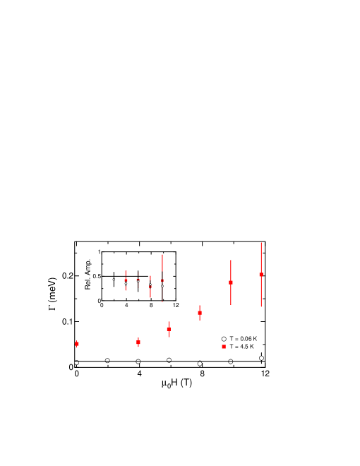
Figure 14: Characteristics of constant energy scans as a function of applied magnetic field at $T=0.06$ K (open symbols) and $T=4.5$ K extracted through Gaussian fits. Representative scans are shown in figure 10. (a) Average resolution corrected half width at half maximum for finite energy modes. Inset shows the ratio of integrated intensities for the field dependent modes to the central field independent mode. The solid line indicates the theoretical ratio of 0.5 expected for $H<H_{c1}$ at $T=0$.

We use inelastic neutron scattering to examine the crossover between the low-field gapped (QP) and gapless (RC-2D) portions of the phase diagram. The $T=0.06$ K lower critical field determined by comparing the peak locations in low-temperature constant energy scans to Eq. LABEL:eq:fandisp is plotted in figure 11(a) and (b) (solid diamond at $T=0.06$ K). With wave vector transfer at ${\mathbf{Q}}=(\frac{1}{2}0\bar{\frac{1}{2}})$ and energy transfer fixed at $\hbar\omega=0.3$ meV the data in figure 15 show the field dependent intensity for various fixed temperatures. At the lowest temperature a sharp peak indicates the field at which the $S_{z}=1$ mode passes through the 0.3 meV energy window of the detection system. With increasing temperature and hence increasing magnon density not only does the peak broaden as expected from an increased relaxation rate, it also moves to higher fields indicating a finite slope for the crossover line in the $H-T$ plane. Just as for the finite magnon lifetime, the origin of this effect is magnon repulsion. The increasing background is likely due to population of low-energy gapless excitations which develop for magnetic fields above the lower critical field. By extrapolation to the $\hbar\omega=0$ line in Fig. 15(b), these data were used to determine the temperature dependence of the field required to close the spin gap and the corresponding data points are included in figure 11(a) and (b) (solid diamonds). The coincidence between the crossover field determined in this manner and the fields associated with differential susceptibility anomalies establish a not unexpected association between effectively closing the gap at the critical wave vector and maximizing the differential uniform susceptibility.

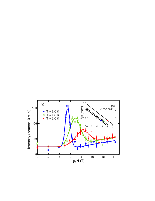
Figure 15: (a) Inelastic neutron scattering intensity at $\hbar\omega=0.3$ meV and $(\frac{1}{2}0\bar{\frac{1}{2}})$ as a function of applied magnetic field, ${\bf H}\parallel{\mathbf{b}}$. Solid lines are the result of a global fit to a Gaussian peak with a sloping background above the magnetic field $H_{0}$ and a constant background below the magnetic field $H_{0}$. Values of the constant background, $H_{0}$, and slope were global parameters in the fit. (b) Energy transfer versus magnetic field for peak locations as determined from (a) and the $T=4.5$ K and $T=0.06$ K data in figure 10(a). Symbols used in (b) correspond to those used in (a). Solid lines are fits to lines as described in the text. The extrapolated intercepts define an effective temperature dependent crossover field.

4.4.2 Magnetic Excitations in the high field paramagnetic state

The previous results indicate a well defined crossover in PHCC from a low field and low temperature state dominated by a gap in the excitation spectrum to a high field state with an excitation spectrum that has finite spectral weight at zero energy. The crossover clearly occurs at lower fields than required to induce long range magnetic order. There are possible analogies to certain $S=1/2$ 1D Heisenberg antiferromagnetic systems including the linear chain, the next nearest neighbor frustrated chain, and the alternating chain where a low-energy continuum of excitations is predicted to exist upon closure of the spin-gap [45, 46, 47]. Calculations examining both gapped and gapless $S=1/2$ spin-orbital chains describe an incommensurate gapless continuum for large portions of exchange and orbital interaction parameter space [48]. A characteristic of these continua are soft incommensurate modes moving through the Brillouin zone from the antiferromagnetic zone center to the ferromagnetic point as a function of applied magnetic field [31, 49, 50, 51]. Incommensurate magnetic field dependent soft modes are also found in numerical calculations for the 2D antiferromagnetic square lattice with next nearest neighbor interactions, a system with similar antiferromagnetic interactions as PHCC [34].

An important distinction between PHCC and the systems mentioned above lies in the fact that for PHCC the putative gapless state so far was only observed at finite temperatures. Ascribing this to the inevitable effects of inter-plane coupling, the analogue of which occurs via interchain coupling in quasi-one-dimensional systems, there exists a potential for field induced incommensurate correlations in PHCC. Here we present preliminary experiments at the highest fields presently accessible to neutron scattering. The field was $\mu_{0}H=14.2$ Tesla and the temperature chosen was $T=4.5$ K, which is 20% above the critical temperature at that field ($T_{C}(\mu_{0}H=14.2$ T)=3.705(3) K). Shown in Fig. 16 (a) are difference data indicating excess magnetic spectral weight at the antiferromagnetic zone center $(\frac{1}{2}0\bar{\frac{1}{2}})$ as compared to $(\frac{1}{2}0\bar{1})$. The solid line shows a fit to the following resolution convolved Lorentzian relaxation spectrum,

$$S(\omega)\propto\frac{1}{1-\exp(-\beta\hbar\omega)}\frac{\chi_{0}\Gamma\omega}{\Gamma^{2}+\omega^{2}},$$ (2g)

which obeys detailed balance and features a relaxation rate, $\hbar\Gamma=0.025\pm 0.2$ meV. The spectrum extends to and is approximately symmetric about zero energy, which is consistent with a 2D renormalized classical phase close to the phase transition to commensurate magnetic order.

Figure 16 (b) shows two constant energy scans at $\hbar\omega=0.36$ meV and $\hbar\omega=0.55$ meV that indicate short range commensurate magnetic correlations. The fitted Lorentzian peaks, which are much broader than the experimental resolution (solid bar) correspond to a dynamic correlation length scale of $3.2\pm 2.5$ Å and $4.2\pm 2.1$ Å for the $\hbar\omega=0.55$ meV and $\hbar\omega=0.36$ meV measurement respectively. The magnetization of PHCC is only 20% of the saturation magnetization in these measurements so any incommensurate shift, which should be a similar fraction of the distance to the Brillouin zone center is not clearly visible in the present data.

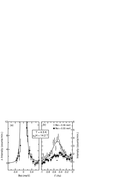
Figure 16: (a) Magnetic inelastic scattering from PHCC at the critical wave vector $(\frac{1}{2}0\bar{\frac{1}{2}})$ for $\mu_{0}H=14.2$ Tesla and $T=4.5$ K which is immediately outside the long range ordered phase. A presumed non-magnetic background measured at $(\frac{1}{2}0\bar{1})$ has been subtracted. The solid line is a fit to a Lorentzian relaxation function as described in the text. (b) Constant energy scans, $\hbar\omega=0.36$ meV, along the $(\frac{1}{2}0l)$ direction at $T=4.5$ K and $\mu_{0}H=14.2$ T for $\hbar\omega=0.36$ and $0.55$ meV. Solid lines through data are fits to a single peaked Lorentzian functions with sloping backgrounds

4.5 Bose condensation of magnons

In this section the phase transition to long range magnetic order in PHCC is analyzed from the perspective of magnon condensation [52, 53, 54, 55]. Following Nikuni et al. [54] and Misguich and Oshikawa [56] we treat magnons as bosons whose density $n$ is proportional to the deviation of the longitudinal magnetization from its plateau value $M_{z0}$: $g\mu_{B}n=|M_{z}-M_{z0}|$. The low-density magnon gas is described by the Hamiltonian

$$\mathcal{H}=\sum_{\mathbf{k}}(\epsilon_{\mathbf{k}}-\mu)a^{\dagger}_{\mathbf{k}}a_{\mathbf{k}}+\frac{v_{0}}{V}\sum_{\mathbf{q,k,k^{\prime}}}a^{\dagger}_{\mathbf{q+k^{\prime}}}a^{\dagger}_{\mathbf{q-k^{\prime}}}a_{\mathbf{q-k}}a_{\mathbf{q+k}},$$ (2h)

where $\mu=g\mu_{B}(H-H_{c1})$ is the boson chemical potential and $v_{0}$ is a short-range repulsion. The energy dispersion $\epsilon_{\mathbf{k}}$ is assumed to have the global minimum at $\mathbf{k}_{0}=[\frac{1}{2}0\frac{1}{2}]$. For convenience, excitation energies are measured from the bottom of the band, so that $\epsilon_{\mathbf{k}_{0}}=0$.

At zero temperature the system acquires a condensate $\langle a_{0}\rangle=\alpha\sqrt{V}$ when $\mu>0$. The energy density of the ground state in the presence of a condensate (neglecting quantum corrections) is $v_{0}|\alpha|^{4}-\mu|\alpha|^{2}$, which is minimized when $|\alpha|^{2}=\mu/2v_{0}$. In this approximation the boson density is

$$n=|\alpha|^{2}=g\mu_{B}(H-H_{c0})/2v_{0}.$$ (2i)

$n$ is related to the longitudinal magnetization

$$M_{z}=g\mu_{B}n$$ (2j)

At a finite temperature we obtain an effective Hamiltonian

$$\mathcal{H}=\sum_{\mathbf{k}}(\epsilon_{\mathbf{k}}-\mu+v_{0}n)a^{\dagger}_{\mathbf{k}}a_{\mathbf{k}},$$ (2k)

where $n$ is the density of thermally excited bosons. The bosons condense when the renormalized chemical potential $\tilde{\mu}\equiv\mu-2v_{0}n$ vanishes. This yields the critical density

$$n_{c}(T)=\frac{1}{V}\sum_{\mathbf{k}}\frac{1}{\exp{({\epsilon_{\mathbf{k}}/T})}-1}.$$ (2l)

The critical field is then

$$H_{c}(T)=H_{c}(0)+2v_{0}n_{c}(T)/g\mu_{B}.$$ (2m)

The boson scattering $v_{0}$ can be extracted from low-temperature magnetization curves. The magnon density per unit cell $n$ is equal to the ratio $M/M_{\mathrm{sat}}$ (there is exactly one magnon per unit cell when $M=M_{\mathrm{sat}}$). Based on the magnetization curve at the lowest available temperature $T=0.46$ K we obtain $v_{0}=1.91$ meV $\times$ the unit-cell volume (u.c.v.). In other words, if we model the magnons as bosons on a cubic lattice with anisotropic hopping and on-site interactions $U$, the interaction strength would be $U=2$ meV. The linear behavior extends over a range of some 10 T, or 13 K in temperature units.

Using this value of the boson coupling we can test the predicted relation between the critical field and critical magnon density (2m) at finite temperatures from the data for $n=M/M_{\mathrm{sat}}$ in the temperature range 0.46 K $\leq T\leq 6$ K. From these we extracted pairs $(M,H)$ whose $H(T)$ values were sufficiently close to the line of phase transitions $H_{c}(T)$. The resulting graph is shown in Fig. 17. The zero-temperature critical field $H_{c1}=7.41$ T was determined from the onset of Neel order at the lowest temperatures ($T<0.3$ K). The agreement with Eq. (2m) is fair.

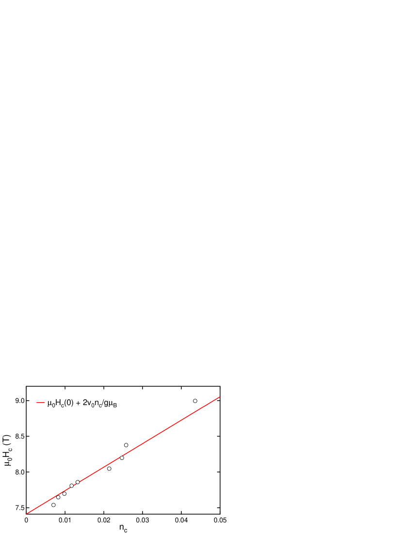
Figure 17: Critical field $H_{c}$ versus critical magnon number per unit cell $n_{c}$. The straight line is Eq. 2m with $\mu_{0}H_{c}(0)=7.41$ T and $v_{0}=1.9$ meV u.c.v.

The line $H_{c}(T)$ is obtained from Eqs. (2l) and (2m). The magnon dispersion is taken from Stone et al. [24] (the 6-term version). That dispersion relation $\epsilon_{\mathbf{k}}^{\mathrm{2D}}$ is strictly two-dimensional, which precludes Bose condensation at a finite temperature. We therefore added weak tunnelling between the planes:

$$\epsilon_{\mathbf{k}}=\epsilon_{\mathbf{k}}^{\mathrm{2D}}+2\tau[1-\cos{(k_{y}b)}].$$ (2n)

The experimental data [57] give an upper bound for the total bandwidth in the $[010]$ direction: $4\tau<0.5$ meV.

When $T\ll\tau$, only the bottom of the magnon band has thermal excitations and one may replace the exact band structure with a parabolic dispersion to obtain

$$n_{c}(T)=\zeta(3/2)\,\left(\frac{m^{\mathrm{3D}}T}{2\pi\hbar^{2}}\right)^{3/2},$$ (2o)

where $m^{\mathrm{3D}}=(m_{a}m_{b}m_{c})^{1/3}$ is the 3D effective mass. In the limit of a very weak interplane tunnelling we can also access a regime where $\tau\ll T\ll W$, where $W\approx 2$ meV is the magnon bandwidth. In this regime the in-plane dispersion can still be treated as parabolic. This yields the critical density for a quasi-2D Bose gas [58]

$$n_{c}(T)=\frac{m^{\mathrm{2D}}T}{2\pi\hbar^{2}b}\,\log{\frac{2T}{\tau}},$$ (2p)

where $m^{\mathrm{2D}}=(m_{a}m_{c})^{1/2}$ and $b$ is the interplane distance. In the intermediate regime $T=\mathcal{O}(\tau)$ the critical density first rises faster than $T^{3/2}$ [56] before crossing over to the $T\log{T}$ behavior.

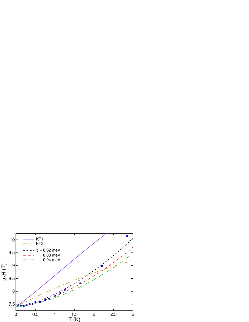
Figure 18: Squares are data for $H_{c}(T)$ from elastic neutron scattering. $H_{c1}(T=0)=7.41$ T, $v_{0}=1.91$ meV u.c.v. Solid lines are discussed in the text.

Curves for $n_{c}(T)$ were obtained by integrating Eq. (2l) numerically for several values of the interplane tunnelling $\tau$. Since $v_{0}$ is already fixed, there are no further adjustable parameters. The data below 2.5 K ($H_{c}<9$ T, $n_{c}<0.05$ per unit cell) are best described by the curves for $\tau=0.03(1)$ meV. The results are shown in Fig. 18.

The theory based on the Hamiltonian (2k) assumes that the boson interaction $v_{0}$ is weak. However, it is also applicable to strongly interacting bosons, as long as the interaction is short-range and the gas is sufficiently dilute. In that case $v_{0}$ is not the bare interaction strength (which can be large) but rather the scattering amplitude (the t-matrix) for a pair of low-energy bosons. For hard-core bosons on a cubic lattice with a nearest-neighbor hopping amplitude $t$, one obtains $v_{0}\approx 8t$ [59]. In our case $t\approx W/8=0.25$ meV giving $v_{0}\approx 2$ meV. Another estimate along these lines, using the “exact” magnon dispersion yields, via

$$\frac{1}{v_{0}}=\frac{1}{V}\sum_{\mathbf{k}}\frac{1}{2\epsilon_{\mathbf{k}}},$$ (2q)

yields a similar value of $v_{0}=2.5$ meV. These numbers demonstrate that the inferred interaction strength of 1.91 meV u.c.v. is quite reasonable.

At higher temperatures the agreement worsens. At $T=3.7$ K—the highest temperature where the condensation is observed—the mean-field theory predicts $H_{c}=11$ T, well below the observed value of 14.2 T. The observed magnon density at the critical field is 0.19 per unit cell (the theoretical estimate is 0.10). It is possible that the mean-field theory of magnon condensation, appropriate for a dilute Bose gas of magnons, becomes unreliable due to overcrowding. (At a technical level, the assumption of pairwise interactions may break down: two particles no longer collide in a vacuum.) Another possible reason for this failure is an increased strength of (thermal) critical fluctuations.

4.6 Kosterlitz-Thouless scenario

If the planes in PHCC were fully decoupled from each other the Bose condensation would change into the Kosterlitz-Thouless (KT) vortex-unbinding transition. It does not seem likely that the data can be reconciled with this scenario: in $d=2$ spatial dimensions the crossover exponent $\phi=1$, so that the line of KT transitions $H_{c}(T)=H_{c}(0)+CT^{\phi}$ is expected to be linear.

The quantum criticality of the two-dimensional Bose gas was recently examined by Sachdev and Dunkel [60] who used a combination of scaling arguments and numerics to determine $H_{c}(T)$ for a weakly interacting Bose gas (2k). (Analyzing the RG flow alone does not solve the problem: the KT fixed point lies in a strongly coupled limit.)

The RG analysis focuses on two variables: the (renormalized) chemical potential $\tilde{\mu}$ and the two-particle scattering amplitude $v$. Unlike in $d=3$ dimensions, the scattering amplitude vanishes in the limit of zero energy. Therefore the role of the coupling constant is played by the t-matrix for particles with energies $\mathcal{O}(T)$:

$$v=\frac{4\pi\hbar^{2}}{m\log{(\Lambda/T)}},$$ (2r)

where $\Lambda$ is a high-energy cutoff on the order of the magnon bandwidth.

While both $\tilde{\mu}$ and $v$ flow under RG transformations, a certain combination of these variables, namely $Tv/\tilde{\mu}$, remains unchanged. The value of this constant determines whether the system flows to the disordered phase or to the phase with long-range correlations. The KT transition corresponds to

$$\frac{2mTv}{\hbar^{2}\tilde{\mu}}=-K\approx-34.$$ (2s)

At the KT transition, the renormalized chemical potential is

$$\tilde{\mu}=-\frac{8\pi}{K\log{(\Lambda/T)}}T.$$ (2t)

We see that $|\tilde{\mu}|$ is a bit below $T$ (particularly if $T\ll\Lambda$), which means that there are many thermally excited particles.

The magnetic field is connected to the bare chemical potential:

$$g\mu_{B}(H-H_{c0})=\mu=\tilde{\mu}+2vn.$$ (2u)

The density is computed for an ideal gas:

$$n=\int\frac{d^{2}k}{(2\pi)^{2}}\frac{1}{e^{(\hbar^{2}k^{2}/2m-\tilde{\mu})/T}-1}=\frac{mT}{2\pi\hbar^{2}}\log{\frac{1}{1-e^{\tilde{\mu}/T}}}\approx\frac{mT}{2\pi\hbar^{2}}\log{\frac{T}{-\tilde{\mu}}}.$$ (2v)

This yields the final result for $H_{c}(T)$:

$$g\mu_{B}(H-H_{c0})=\mu=\frac{4T}{\log{(\Lambda/T)}}\left[\log{\left(\frac{K}{8\pi}\log{\frac{\Lambda}{T}}\right)}-\frac{2\pi}{K}\right].$$ (2w)

It depends weakly on the ultraviolet cutoff $\Lambda$. For $\Lambda=2.5$ meV, we have $\mu\approx 1.5T$ in the temperature range of interest. The curve is labelled ’KT1’ in Fig. 18.

The result (2w) can also be obtained directly from Eqs. (3) and (4) of Sachdev and Dunkel [60] if one takes the classical limit $\mu\ll T$. The value $\mu\approx 1.5T$ suggests that we are (just) outside the classical regime and one needs to solve the Sachdev-Dunkel equations numerically. The resulting curve (for $\Lambda=2.5$ meV) is shown in Fig. 18 as ’KT2’. It is also approximately linear, with a slope $d\mu/dT\approx 1$.

Even with the refined approach, the KT theory does not seem to agree with the data. As anticipated, it produces a linear dependence $H_{c}(T)$ (up to logarithmic corrections) instead of a higher power law. The rise of the data above the KT line at high temperatures may signal the inadequacy of the continuum approximation at high magnon concentrations.

5 Conclusions

Originally thought to be a weakly alternating spin chain, our measurements establish PHCC as a quasi-two-dimensional spin-dimer system. The gap is sufficiently small to allow access to the lower critical field and the bandwidth sufficiently large to produce several distinct phases.

The long range Néel ordered phase is a commensurate antiferromagnet with moments perpendicular to the applied field direction. The critical exponents for the phase transition are similar to those of a 3D Ising model. The transition into this phase can be described as magnon Bose-Einstein condensation. Mean-field (Hartree-Fock) theory does an adequate job describing the magnetization $M(H)$ at the lowest temperatures ($T=0.46$ K) and the shape of the critical line $H_{c}(T)$ for $T<3$ K. The theory predicts a small but nonzero magnon dispersion of $0.08\geq 4\tau\leq 0.16$ meV perpendicular to the 2D planes. The higher power of the $H_{c}(T)$ dependence is caused by deviations of the magnon density of states from the $E^{1/2}$ behavior of the continuum theory. The extra DOS (due to a van Hove singularity) is positive, hence an increase over the $T^{3/2}$ law. The continuum KT theory gives an approximately linear dependence $H_{c}(T)$ and thus does not seem to do a good job.

Close to the lower quantum critical point there is an anomaly in the phase boundary that is not accounted for by the BEC theory (see figure 11(b) and figure 9(a)-(c).) Low T anomalies near the zero temperature termination of phase boundaries are also seen experimentally in the quantum liquids ³He[61] and ⁴He[62, 63], the frustrated spin system GGG[7, 8], and in numerical and theoretical results for the BCC Ising antiferromagnet [64], the Ising antiferromagnet on a cubic lattice [65], and $S=1/2$ XXZ 1D- [66] and 2D- [67] antiferromagnets. In ⁴He the anomaly is associated with there being more low energy degrees of freedom in the solid than the liquid and a low$-T$ anomaly in the phase boundary of LiHoF₄ has been associated with nuclear spin degrees of freedom.[68] For PHCC we speculate that features beyond a spin model such as the relatively soft lattice or nuclear spins become relevant sufficiently close to the quantum critical point. Such a mechanism which appears to be rather general merits further exploration through experiments that probe such auxiliary degrees of freedom directly.

The high field paramagnetic phase is perhaps the most intriguing aspect of PHCC. The crossover from the quantum paramagnet to this phase remains remarkably sharp upon heating and the experiments show that a finite temperature pseudo spin gap closes there. Further analysis is required to understand why this crossover remains so distinct. A proper examination of the gapless high field phase requires inelastic neutron scattering magnetic fields of order 30 Tesla where the system is more heavily magnetized. This work must await development of a higher field facility for inelastic neutron scattering.

References

References

- [1] Miller J S (ed) 1983 Extended Linear Chain Compounds (New York: Plenum) and references therein
- [2] de Jongh L J and Miedema A R 1974 Adv. in Phys. 23 1, and references therein
- [3] Broholm C and Aeppli G (2004), in ”Strong Interactions in Low Dimensions (Physics and Chemistry of Materials With Low Dimensional Structures)”, Baeriswyl D and Degiorgi L, Eds. Kluwer ISBN: 1402017987, Chapter 2, page 21
- [4] Broholm C, Aeppli G, Chen Y, Dender D C, Enderle M, Hammar P R, Honda Z, Katsumata K, Landee C P, Oshikawa M, Regnault L P, Reich D H, Shapiro S M, Sieling M, Stone M B, Turnbull M M, Zaliznyak I, and Zheludev A (2002), in High Magnetic Fields applications in condensed matter physics and spectroscopy C. Berthier, L. P. Lévy, and G. Martinez, Eds. Springer Verlag, p 211-234
- [5] Broholm C, Reich D H, Aeppli G, Lee S-H, Dender D, Hammar P, Xu G, DiTusa J F, and Ramirez A P (1998) in ”Dynamical Properties of Unconventional Magnetic Systems edited by Skjeltorp A T and Sherrington D, NATO ASI Series, Series E: Applied Sciences vol. 349, Kluwer Academic Publishers, Boston 77
- [6] Landau L D (1933) Phys. Zeit. Sov. 4 675
- [7] Ramirez A P and Kleiman R N (1991) J. Appl. Phys. 69 5252
- [8] Tsui Y K, Burns C A, Snyder J and Schiffer P (1999) Phys. Rev. Lett. 82 3532
- [9] Stone M B, Chen Y, Rittner J, Yardimci H, Reich D H and Broholm C (2002) Phys. Rev. B 65 64423
- [10] Leuenberger B, Güdel H U, Feile R and Kjems J K (1985) Phys. Rev. B 31 597
- [11] Oosawa A, Tanaka H, Takamasu T, Abe H, Tsujii N and Kido G (2001) Physica B 294-295 34
- [12] Oosawa A, Ishii M and Tanaka H (1999) J. Phys.: Condens. Matter 11 265
- [13] Cavadini N, Heigold G, Hennggeler W, Furrer A, Güdel H -U, Krämer K and Mutka H (2001) Phys. Rev. B 63 172414
- [14] Rüegg Ch, Cavadini N, Furrer A, Güdel H-U., Mutka H, Wildes A, Habicht K and Vorderwisch P (2003) Nature 423 62
- [15] Stone M B, Chen Y, Xu G, Reich D H, Broholm C, Copley J and Cook J unpublished, see also [57].
- [16] Xu G, Broholm C, Reich D H and Adams M A 2000 Phys. Rev. Lett. 84 4465
- [17] Calvo R, Passeggi M C G, Moreno N O, Barberis G E, Chaves A B, Torres B C M, Lezama L and Rojo T 1999 Phys. Rev. B 60 1197
- [18] Hong T, Turnbull M M, Landee C P, Schmidt K P, Uhrig G S, Qiu Y, Broholm C, and Reich D H (2006) Phys. Rev. B 74
- [19] Shapiro A, Landee C P, Turnbull M M, Jornet J, Deumal M, Novoa J J, and Lewis W (2006) to appear in J. Am. Chem. Soc.
- [20] Sasago Y, Uchinokura K, Zheludev A and Shirane G (1997) Phys. Rev. B 55 8357
- [21] Sebastian S E, Harrison N, Batista C D, Balicas L, Jaime M, Sharma P A, Kawashima N and Fisher I R (2006) Nature 441 617.
- [22] Kageyama H, Nishi M, Aso N, Onizuka K, Yosihama T, Nukui K, Kodama K, Kakurai K and Ueda Y (2000) Phys. Rev. Lett. 84 5876
- [23] Y. Hosokoshi, Y. Nakazawa and K. Inoue, Phys. Rev. B 60, 12924 (1999).
- [24] Stone M B, Zaliznyak I A, Reich D H and Broholm C (2001) Phys. Rev. B 64 144405
- [25] Stone M B, Zaliznyak I A, Hong T, Reich D H and Broholm C L (2006) Nature 440 187
- [26] Battaglia L P, Corradi A B, Geiser U, Willett R, Motori A, Sandrolini F, Antolini L, Manfredini T, Menaube L and Pellacani G C (1988) J. Chem. Soc. Dalton Trans. 2 265
- [27] Stone M B, Broholm C, Reich D H, Tchernyshyov O, Vorderwisch P and Harrison N (2006) Phys. Rev. Lett. 96 257203
- [28] Daoud A, Ben Salah A, Chappert C, Renard J P, Cheikhrouhou A, Duc T and Verdaguer M (1986) Phys. Rev. B 33 6253
- [29] Ma S, Broholm C, Reich D H, Sternlieb B J, and Erwin R W (1992) Phys. Rev. Lett. 69, 3571
- [30] Wang X and Yu L (2000) Phys. Rev. Lett. 84 5399
- [31] Chitra R and Giamarchi T (1997) Phys. Rev. B 55 5816
- [32] Sakai T and Takahashi M (1998) Phys. Rev. B 57 R8091
- [33] Zhitomirsky M E and Nikuni T (1998) Phys. Rev. B 57 5013
- [34] Yang M S and Mütter K H (1997) Z. Phys. B 104 117
- [35] Gu Q and Shen J L (2000) Eur. Phys. J. B 18 63
- [36] Collins M (1989) Magnetic Critical Scattering (USA: Oxford University Press)
- [37] Campostrini M, Hasenbusch M, Pelissetto A, Rossi P and Vicari E (2002) Phys. Rev. B 65 144520
- [38] Campostrini M, Hasenbusch M, Pelissetto A, Rossi P and Vicari E (2001) Phys. Rev. B 63 214503
- [39] Campostini M, Pelissetto A, Rossi P, Vicari E (1999) Phys. Rev. E 60 3526
- [40] Chesser N D and Axe J D (1973) Acta Crystallogr. Sect. A 28 160
- [41] Lovesey S W 1984 Theory of Neutron Scattering from Condensed Matter (USA: Oxford University Press)
- [42] Squires G L 1978 Introduction to the Theory of Thermal Neutron Scattering (Mineola, NY: Dover)
- [43] Goldenfeld N (1992) Lectures on Phase Transitions and the Renormalization Group (Reading, Massachusets: Perseus Books)
- [44] Rüegg C, Normand B, Matsumoto M, Niedermayer C, Furrer A, Kramer K W, Gudel H U, Bourges P, Sidis Y Mutka H (2005) Phys. Rev. Lett. 95 267201
- [45] Müller G, Thomas H, Beck H and Bonner J C (1981) Phys. Rev. B 24 1429
- [46] Yu W and Haas S (2000) Phys. Rev. B 62 344
- [47] Haga N and Suga S (2001) Phys. Rev. B 65 14414
- [48] Yu W and Haas S (2000) Phys. Rev. B 63 24423
- [49] Tsvelik A M (1995) Quantum Field Theory in Condensed Matter Physics (Cambridge, England: Cambridge University Press)
- [50] Batista C D and Ortiz G (2001) Phys. Rev. Lett. 86 1082
- [51] Wang Y R (1992) Phys. Rev. B. 46 151
- [52] Matsubara T, Matsuda H (1956) Prog. Theor. Phys. 16 569
- [53] Affleck I (1990) Phys. Rev. B 41 6697
- [54] Nikuni T, Oshikawa M, Oosawa A, and Tanaka H (2000) Phys. Rev. Lett. 84 5868
- [55] Fisher M P A, Weichman P B, Grinstein G, and Fisher D S (1989) Phys. Rev. B 40 546
- [56] Misguich G and Oshikawa M (2004) J. Phys. Soc. Jpn. 73 3429
- [57] Stone M B (2002) Ph.D. Thesis, Johns Hopkins University
- [58] Micnas R, Ranninger J, and Robaszkiewicz S (1990) Rev. Mod. Phys. 62, 113
- [59] Friedberg R, Lee T D and Ren H C (1994) Phys. Rev. B 50 10190
- [60] Sachdev S and Dunkel E R (2006) Phys. Rev. B 73 085116
- [61] Pomeranchuk I (1950) Zh. Eksp. Teor. Fiz. 20 919
- [62] Cordillo M C and Ceperley D M (1998) Phys. Rev. B 58 6447
- [63] Straty G C and Adams E D (1966) Phys. Rev. Lett. 17 290
- [64] Landau D P (1977) Phys. Rev. B 16 4164
- [65] Hui K (1988) Phys. Rev. B 38 802
- [66] Hieida Y, Okunishi K and Akutsu Y (2001) Phys. Rev. B 64 224422
- [67] Schmid G, Todo S, Troyer M and Dorneich A (2002) Phys. Rev. Lett. 88 167208
- [68] Bitko D, Rosenbaum T F, and Aeppli G (1996) Phys. Rev. Lett. 77 940