Collective Excitations of Dirac Electrons in Graphene

Abstract

Two-dimensional electrons in graphene are known to behave as massless fermions with Dirac-Weyl type linear dispersion near the Dirac crossing points. We have investigated the collective excitations of this system in the presence or absence of an external magnetic field. Unlike in the conventional two-dimensional electron system, the $\nu=\frac{1}{m}$ fractional quantum Hall state in graphene was found to be most stable in the $n=1$ Landau level. In the zero field case, but in the presence of the spin-orbit interaction, an undamped plasmon mode was found to exist in the gap of the single-particle continuum.

I Introduction

In recent experimental work, it has been possible to extract an atomically thin, two-dimensional (2D) sheet of graphite – graphene, by micromechanical cleavagegraphene_2D . A two-dimensional electron system in graphene exhibits many remarkable properties. In the band structure calculations where electrons are treated as hopping on a hexagonal latticewallace , one finds a unique linear (relativistic type) energy dispersion near the corners of the first Brillouin zone where the conduction and valence bands meet. As a consequence, the low-energy excitations follow the Dirac-Weyl equations for massless relativistic particlesando . In an external magnetic field, the spectrum develops into Landau levels, each of which approximately fourfold degeneratemcclure ; landau_levels . Recent discovery of the quantum Hall effect in grapheneqhe_expt ; high_field ; qhe_theory has resulted in intense activitiesphys_today to unravel the electronic properties of graphene that are distinctly different from the conventional (or, as popularly called the ‘non-relativistic’) 2D electron systems in semiconductor structures. In this paper, we report on our investigation of the collective excitations of the 2D electron gas in graphene in the presence or absence of an external magnetic field.

Graphene has a honeycomb lattice structure of $sp^{2}$ carbon atoms, with two atoms, A and B per unit cell (i.e., a two-dimensional triangular Bravais lattice with a basis of two atoms). Each atom is tied with its three nearest neighbors via strong $\sigma$ bonds that are in the same plane with angles of 120^∘. The $\pi$ orbit ($2p_{z}$) of each atom is perpendicular to the plane and overlaps with the $\pi$ orbitals of the neighboring atoms that results in the delocalized $\pi$ and $\pi^{\ast}$ bands. There is only one electron in each $\pi$ orbit and the Fermi energy is located between the $\pi$ and $\pi^{\ast}$ bands. The separation distance between the nearest neighbor atoms is $a_{cc}=0.14$ nm while the lattice constant is $a=\sqrt{3}a_{cc}=0.246$ nm. The dynamics of electrons in graphene is described by a nearest-neighbor tight-binding modelwallace that describes the hopping of electrons between the $2p_{z}$ carbon orbitals. The first Brillouin zone is hexagonal and at two of its inequivalent corners (the K and K^′ points) the conduction and valence bands meet. Graphene is often described as a two valley (K and K^′) zero-gap semiconductor. The two valleys correspond to two chiralities of the Weyl-Dirac fermionschiral . Near these two points (the so-called Dirac points), the electrons have a relativistic-like dispersion relation, $\varepsilon_{k}=\pm\hbar v|{\bf k}|$ and obey the Dirac-Weyl equations for massless fermions. At the vanishing gate voltage, the system is half-filled and the Fermi level lies at the Dirac points.

II Collective modes

In the following sections, we describe results of our work on the collective excitations of electrons in graphene. First, we discuss the case of the collective modes in the presence of a strong perpendicular magnetic field. In particular, we discuss the properties of the fractional quantum Hall states that reflect the nature of electron correlations in the system in the presence of a strong magnetic field. We found that the linear dispersion of electrons discussed above, leads to a noticeable change in the behavior than what is expected in a conventional two-dimensional electron system. In the last section, we discuss the zero-field case using the random-phase approximation and explore the properties of plasmons in such a system.

II.1 In a magnetic field

An external magnetic field has a significant influence on the energy spectrum of the 2D electron system in graphene. Details of the single-electron case has been widely reported in the literatureando ; landau_levels .

II.1.1 Landau levels

In the continuum limit the electron wave function in graphene is a 8-component spinor, $\Psi_{s,k,\alpha}$, where $s=\pm 1/2$ is the spin index, $k=K,K^{\prime}$ is the valley index, and $\alpha=A,B$ is the sublattice index. Without the spin-orbit interactionkane05 ; wang06 ; sini the spin degrees of freedom becomes uncoupled from the spatial motion and the Hamiltonian of an electron can be described by two $4\times 4$ matrices for each component of the electron spin. If we introduce the four-component spinor as $(\Psi_{s,K,A},\Psi_{s,K,B},\Psi_{s,K^{\prime},A},\Psi_{s,K^{\prime},B})$ then in the presence of a magnetic field perpendicular to the graphene plane the Hamiltonian matrix has the form

$${\cal H}=v\left(\begin{array}[]{cccc}0&\pi_{x}-i\pi_{y}&0&0\\ \pi_{x}+i\pi_{y}&0&0&0\\ 0&0&0&\pi_{x}-i\pi_{y}\\ 0&0&\pi_{x}+i\pi_{y}&0\end{array}\right),$$ (1)

where ${\bm{\pi}}$=${\bm{p}}+e{\bm{A}}/c$, $\bm{p}$ is the two-dimensional momentum, $\bm{A}$ is the vector potential, and $v$ is the velocity of electrons in graphene. It is easy to see from the Hamiltonian matrix (1) that the valley index in conserved. The conservation of the valley index is easily violated in the graphene systems with a short-range scattering impurity potential or in the many-body systems with inter-electron interactions. In both cases the scattering of the electron either by an impurity or by another electron introduces the umklapp process and a change of the electron valley index.

Just as for the non-relativistic system the application of a perpendicular magnetic field to the graphene layer results in the Landau quantization. Due to the relativistic nature of electrons in graphene the energy spectrum of the Landau levels has a unique form, namely, the energy of the $n$th Landau level is $E_{n}=sgn(n)\sqrt{2e\hbar v^{2}|n|B}$. This is different from the non-relativistic electrons, where the Landau level spectrum is of the harmonic oscillator type, i.e. equidistant, $E_{n}\propto n$.

In the ideal graphene system the eigenfunctions of the single-electron Hamiltonian (1) are specified by the Landau index, $n=0,\pm 1,\pm 2,\ldots$ and an intra-Landau index $m$, which depends on the gauge. Each Landau level is fourfold degenerate due to the spin and valley degrees of freedom. The corresponding wave functions for an electron in the valleys $K$ and $K^{\prime}$ are described by the vectors

$$\Psi_{K,n}=C_{n}\left(\begin{array}[]{c}{\rm sgn}(n)i^{|n|-1}\phi_{|n|-1}\\ i^{|n|}\phi_{|n|}\\ 0\\ 0\end{array}\right),$$ (2)

$$\Psi_{K^{\prime},n}=C_{n}\left(\begin{array}[]{c}0\\ 0\\ i^{|n|}\phi_{|n|}\\ {\rm sgn}(n)i^{|n|-1}\phi_{|n|-1}\end{array}\right),$$ (3)

where $C_{n}=1$ for $n=0$ and $C_{n}=1/\sqrt{2}$ for $n\neq 0$. The two non-zero terms in $\Psi_{K,n}\,(\Psi_{K^{\prime},n})$ correspond to occupation of the sublattice A (the upper term) and the sublattice B (the lower term). Here $\phi_{n}$ is the Landau wave function for a particle with the non-relativistic parabolic dispersion relation in the $n$-th Landau level. From Eqs. (2)–(3) it is clear that a specific feature of the relativistic dispersion law is the “mixture” of the non-relativistic Landau levels. This mixture is present only for $n\neq 0$. For $n=0$ the electron in the valley $K$ or $K^{\prime}$ occupies only the sublattice $A$ or $B$, respectively. For higher Landau levels the electron in each valley occupies both sublattices, $A$ and $B$. The wave functions in the sublattices $A$ and $B$ are the wave functions of the non-relativistic electrons with different Landau level indices, i.e. the relativistic wave function is the mixture of non-relativistic wave functions of different Landau levels. As we shall see below, this property of the relativistic electrons strongly modifies the inter-electron interaction within a single relativistic Landau level.

II.1.2 Inter-electron interaction

In what follows, we shall consider only the partially occupied Landau levels with fractional filling factors. In this case the ground state of the system and the excitation spectrum are fully determined by the inter-electron interactions, which are completely described by the Haldane pseudopotentialshaldane $V_{m}$. Haldane pseudopotentials are the energies of two electrons with relative angular momentum $m$. The pseudopotentials for the $n$-th Landau level can be presented ashaldane

$$V_{m}^{(n)}=\int_{0}^{\infty}\frac{dq}{2\pi}qV(q)\left[F_{n}(q)\right]^{2}L_{m}(q^{2})e^{-q^{2}},$$ (4)

where $L_{m}(x)$ are the Laguerre polynomials, $V(q)=2\pi e^{2}/(\kappa lq)$ is the Coulomb interaction in the momentum space, $\kappa$ is the dielectric constant, and $F_{n}(q)$ is the form factor corresponding to the $n$-th Landau level. The main difference between the relativistic and the non-relativistic electrons is in the expression for the form factor, $F_{n}(q)$. For relativistic electrons the form factor is given by the equationsnomura ; goerbig06

$$F_{0}(q)=L_{0}\left(\frac{q^{2}}{2}\right)$$ (5)

$$F_{n\neq 0}(q)=\frac{1}{2}\left[L_{n}\left(\frac{q^{2}}{2}\right)+L_{n-1}\left(\frac{q^{2}}{2}\right)\right],$$ (6)

while for the non-relativistic particles the form factors in Eq. (4) are

$$F_{n}(q)=L_{n}\left(q^{2}/2\right).$$

Comparing these non-relativistic form factors [Eq. (II.1.2)] with Eqs. (5)-(6), we see that the inter-electron interactions for the relativistic and the non-relativistic electrons are the same for $n=0$ and different for $n>0$.

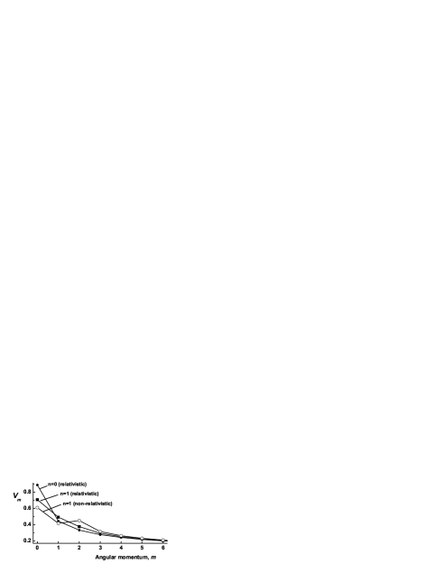
Figure 1: Pseudopotentials calculated from Eq. (4) are shown as a function of the relative angular momentum for relativistic and non-relativistic 2D electrons for the first two Landau levels. The energy is measured in units of $\epsilon_{C}$.

In Fig. 1 the pseudopotentials calculated from Eq. (4) for the relativistic and the non-relativistic cases are shown. For $n=0$ the non-relativistic and the relativistic pseudopotentials are the same. The main feature of the pseudopotentials in the zeroth Landau level, $V_{m}^{(0)}$, is their monotonic decrease with increasing relative angular momentum, $m$. Comparing $V_{m}^{(0)}$ to the non-relativistic $V_{m}^{(1)}$ we can clearly see that (i) in higher Landau levels the pseudopotentials become a non-monotonic function of $m$ and (ii) the interaction strength is suppressed at $m=0$ and 1, i.e. $V_{m}^{(1)}<V_{m}^{(0)}$, and enhanced at $m>1$, i.e. $V_{m}^{(1)}>V_{m}^{(0)}$. From this behavior we can make the predictions about the stability and excitation gaps of the FQHE. For example, for the $\nu=1/3$-FQHE the main parameter which determines the formation the incompressible liquid is the ratio of the pseudopotentials at $m=3$ and $m=1$, i.e., $V_{3}/V_{1}$. The smaller the ratio the larger the excitation gaps, and consequently the more stable are the FQHE states. Comparing the pseudopotentials of the non-relativistic electrons at $n=1$ and $n=0$ we can conclude that the FQHE gaps in the first Landau level, $n=1$ should be smaller then the corresponding gaps in the zeroth Landau level, $n=0$.

The behavior of the pseudopotentials for the relativistic electrons in the higher Landau levels is similar to that of the relativistic ones. The exception is the properties of the pseudopotential in the first Landau level, $n=1$. We notice in Fig. 1 that the pseudopotentials in the first Landau level ($n=1$) is larger than the corresponding pseudopotentials in the zeroth Landau level, $n=0$, for all values of the relative angular momentum, i.e. $V_{m}^{(1)}>V_{m}^{(0)}$. The pseudopotential in the $n=1$ Landau level is also a monotonic function of $m$. This is different from the non-relativistic case. Another important property of the pseudopotential of the relativistic system is that the ratio $V_{3}/V_{1}$ is the smallest in the first Landau level, $n=1$. In Fig. 2 we present the results for the pseudopotentials of the relativistic system in the lowest Landau levels. From this figure we can also see that the ratio $V_{3}/V_{1}$ is the smallest for $n=1$. Based on this property of $V_{m}^{(n)}$ we can conclude that the largest gap of the 1/3-FQHE state should be expected in the first Landau level, $n=1$. Therefore the FQHE in the relativistic system should be easier to observe in the first Landau level, but not in the zeroth Landau level as in the case of the non-relativistic electrons.

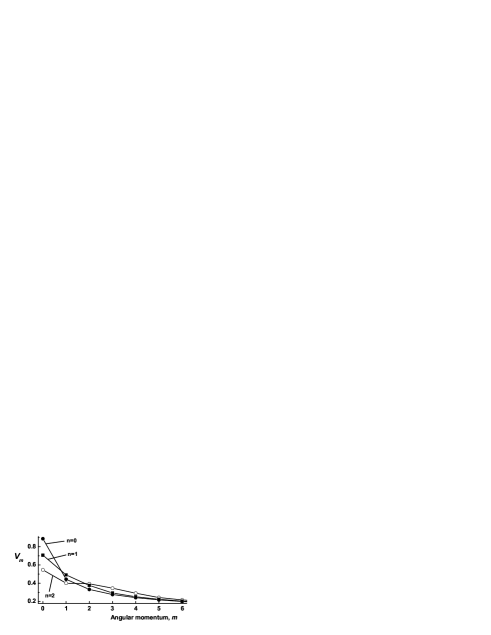
Figure 2: Pseudopotentials are shown as a function of the relative angular momentum for relativistic electrons in the first three lowest Landau levels. The energy is measured in units of $\epsilon_{C}$.

Due to the presence of both the spin and the valley degeneracies the graphene system becomes more complicated than the standard non-relativistic electron system, where only the spin degree of freedom is present. In a magnetic field the spin degeneracy can be lifted due to the Zeeman energy, leaving the Landau levels of the graphene system doubly degenerate due to the valley index. Mathematically, the system then becomes equivalent to a double layer non-relativistic system, where the valley index is the layer index. Usually, in the double-layer system there is an asymmetry in the interaction Hamiltonian. This means that the interaction strength between the electrons in the same layers is different from that in different layers. This is due to a finite separation between the layers. Comparing this property of a double layer system to the graphene system we can say that the graphene system is a double-layer system with zero separation between the layers. So the system is completely SU(2)-pseudospin symmetric, where the pseudospin is associated with the valley index. But this is not entirely true. There is an asymmetry in the graphene system as well. One of the types of asymmetry is related to the lattice structure of graphene — the interaction between the electrons in the same sublattice is stronger than the interaction between the electrons in different sublatticesfisher06 .

To estimate the corrections due to the asymmetry related to the lattice structure of graphene we assume that the electrons are localized at the discrete points corresponding to the lattice structure of the graphene. Then the interaction matrix element, $V_{i_{1},j_{1},i_{2},j_{2}}$, between the single-electrons states, $\psi_{i}$, can be expressed in the following form

$$V_{i_{1},j_{1},i_{2},j_{2}}=\sum_{{\bf r}_{1}}\sum_{{\bf r}_{2}}\psi^{*}_{i_{1}}({\bf r}_{1})\psi^{*}_{j_{1}}({\bf r}_{2})V({\bf r}_{1}-{\bf r}_{2})\psi_{j_{2}}({\bf r}_{2})\psi_{i_{2}}({\bf r}_{1})$$ (7)

where the index $i$ in the wavefunction $\psi_{i}$ indicates collectively the Landau level, valley, sublattice, and intra-Landau level indices. The sums in (7) run over the discrete positions of the electrons corresponding to one of the sublattices of graphene. In the continuum limit the sums should be replaced by the integral. Since two sublattices of graphene are shifted by the vector ${\bf r}_{0}=a(0,1/\sqrt{3})$, in the continuum limit the expression for the interaction matrix element between the states belonging to different sublattices should contain not the $V({\bf r}_{1}-{\bf r}_{2})$ but $V({\bf r}_{1}-{\bf r}_{2}-{\bf r}_{0})$. This introduces the difference in the interaction strength between the electrons in the same sublattice and in different sublattices. In terms of the pseudopotentials this means that if the pseudopotential is calculated between the states of different sublattices then $V(q)$ in the expression (4) should contain an additional factor $\exp({i{\bf q}\cdot{\bf r}_{0}})$ and the integral over $q$ should be replaced by the 2D integral over $\bf{q}$.

In the zeroth Landau level, $n=0$, the electrons in the valley $K$ occupy sublattice $A$ only, while the electrons in the valley $K^{\prime}$ occupy sublattice $B$. Then the pseudopotentials corresponding to the interaction between the electrons belonging to the same valley are given by the expression (4) without any modifications. The expression for the pseudopotentials corresponding to the interaction between the electrons in the different valleys should contain an additional factor and can be written as

$$V_{K,K^{\prime},m}^{(0)} = \int\frac{d{\bf q}}{4\pi^{2}}V(q)e^{i{\bf q}\cdot{\bf r}_{0}/l}L_{m}(q^{2})e^{-q^{2}}$$ (8)

$$= V_{K,K,m}^{(0)}-\left(\frac{r_{0}}{l}\right)^{2}\int\frac{q^{2}dq}{4\pi}V(q)L_{m}(q^{2})e^{-q^{2}}.$$

Since $r_{0}=a/\sqrt{3}$ the asymmetric correction is proportional to a small parameter $(a/l)^{2}$.

In the higher Landau levels the electrons in the valleys $K$ and $K^{\prime}$ occupy both sublattices $A$ and $B$. This results in the form factor of $\frac{1}{4}(L_{n}+L_{n-1})^{2}$ in Eq. (4). The coefficients $L_{n}$ and $L_{n-1}$ belong to different sublattices. This can be schematically presented in the following form: (i) for the intravalley interaction, we have

$$\frac{1}{4}\left[L_{n}(A)L_{n}(A)+L_{n-1}(B)L_{n-1}(B)+2L_{n}(A)L_{n-1}(B)\right]$$ (9)

and (ii) for the intervalley interaction,

$$\frac{1}{4}\left[L_{n}(A)L_{n}(B)+L_{n-1}(B)L_{n-1}(A)+2L_{n}(A)L_{n-1}(A)\right].$$ (10)

Then following the same procedure as for the $n=0$ Landau level we obtain the expressions for the pseudopotentials in the higher Landau levels as

$$V_{K,K,m}^{(n)}=V_{K^{\prime},K^{\prime},m}^{(n)}=\int\frac{d{\bf q}}{4\pi^{2}}V(q)L_{m}(q^{2})e^{-q^{2}}\left[F_{n}(q)+\frac{1}{2}L_{n}L_{n-1}\left(e^{i{\bf q}\cdot{\bf r}_{0}/l}-1\right)\right],$$ (11)

and

$$V_{K,K^{\prime},m}^{(n)}=\int\frac{d{\bf q}}{4\pi^{2}}V(q)L_{m}(q^{2})e^{-q^{2}}\left[F_{n}(q)e^{i{\bf q}\cdot{\bf r}_{0}/l}+\frac{1}{2}L_{n}L_{n-1}\left(1-e^{i{\bf q}\cdot{\bf r}_{0}/l}\right)\right].$$ (12)

It is convenient to rewrite the expressions (11) and (12) as

$$\tilde{V}_{K,K^{\prime},m}^{(n)}=\tilde{V}_{K,K,m}^{(n)}-\int\frac{d{\bf q}}{(4\pi)^{2}}V(q)L_{m}(q^{2})e^{-q^{2}}\left[L_{n}-L_{n-1}\right]^{2}\left(1-e^{i{\bf q}\cdot{\bf r}_{0}/l}\right).$$ (13)

Similar to the zeroth Landau level the asymmetry correction in Eq. (13) is proportional to a small parameter $(a/l)^{2}$.

Since the Coulomb interaction between the electrons in graphene does not conserve the valley index there is an other mechanism for violation of the SU(2) valley symmetry of the graphene system. This mechanism is related to the inter-valley scattering. In the lowest order in the small parameter $a/l$ the main scattering process is the backscatteringgoerbig06 . During this process the electron from the $K$ valley is scattered into the $K^{\prime}$ valley, while the electron from the $K^{\prime}$ valley is scattered into the $K$ valley. The interaction matrix elements corresponding to this process are determined by the pseudopotentials (4) where the Coulomb interaction in the integral should be replaced by $V({\bf q}+l\Delta{\bf K})$. Here $\Delta{\bf K}={\bf K}-{\bf K}^{\prime}=(2\pi/a)(-1/3,1/\sqrt{3})$. Therefore the pseudopotentials describing the backscattering process are given by the expression

$$V_{B,m}^{(n)}=\int\frac{d{\bf q}}{4\pi^{2}}V({\bf q}+l\Delta{\bf K})\left[F_{n}(q)\right]^{2}L_{m}(q^{2})e^{-q^{2}}.$$ (14)

The leading order term in $V_{B,m}^{(n)}$ can be found by simply replacing $V({\bf q}+l\Delta{\bf K})$ by $V(l\Delta{\bf K})\propto(a/l)$.

II.1.3 FQHE in graphene

With the pseudopotentials for Dirac electrons at hand, we now evaluate numerically the energy spectra of the many-electron states at the fractional fillings of the Landau level. The calculations have been done in the spherical geometryhaldane with the pseudopotentials given by Eq. (4). In the spherical geometry the radius of the sphere $R$ is related to $2S$ of magnetic fluxes through the sphere in units of the flux quanta as $R=\sqrt{S}l$. Here $2S$ is an integer number. The single-electron states are characterized by the angular momentum $S$, and its $z$ component, $S_{z}$. Therefore, at a given magnetic field, i.e for a given flux $2S$, the number of available states in a sphere is $(2S+1)$. Then for a given number of electrons $N$ the parameter $S$ determines the filling factor of the Landau level. Due to the spherical symmetry of the problem, the many-particle states are described by the total angular momentum $L$ and its $z$ component, while the energy depends only on $L$. The energy spectra of a many-particle system is found by the standard procedure of calculating numerically the lowest eigenvalues and eigenvectors of the interaction Hamiltonian matrixfano .

Figure 3: (a) The energy spectra of an eight-electron $\nu=1/3$-FQHE system shown for different Landau levels: $n=0$ (stars) and $n=1$ (filled circles). The flux quanta is $2S=21$. (b) Energy spectra of the six-electron $\nu=1/5$-FQHE system is shown for different Landau levels: $n=0$ (stars) and $n=1$ (filled circles). The flux quanta here is $2S=25$.

It was shown in the previous section that based on the analysis of the Haldane pseudopotentials we can conclude that the FQHE states in graphene should have the largest gaps in the $n=1$ Landau level. Here we check this statement for $\nu=1/m$ incompressible states. In the spherical geometry, such states are realized at $S=(m/2)(N-1)$. The $1/m$ state in the higher $n$-th Landau level is defined as a state corresponding to the $1/m$ filling factor of the $n$-th Landau level, while all the lower energy Landau levels are completely occupied. If the electron system is fully spin and valley polarized then we should expect that the ground state to be the Laughlin statelaughlin ; fqhe_book which is separated from the excited states by a finite gap.

In Fig. 3(a) the calculated energy spectra are shown for the $1/3$-FQHE state and for different Landau levels. Since the relativistic pseudopotentials, $V_{m}^{(0)}$, for $n=0$ Landau level is similar to that of non-relativistic case, the $1/3$ state and the corresponding energy gap will be the same in both cases. The deviation from the non-relativistic system occurs at the higher Landau levels. From Fig. 3(a) we can clearly see that the energy gap of the $1/3$-state at the $n=1$ Landau level is enhanced when compared to that of the $n=0$ Landau level. At higher Landau levels, i.e., for $n>1$, the excitation gaps are suppressed, which means that at the $n=1$ Landau level the electron system in graphene has the strongest interaction with the largest incompressible gap gr-fqhe . This is different from the non-relativistic case, where the energy gap monotonically decreases with increasing Landau level indexfqhe_book . At other filling factors of the type $\nu=1/m$ we should also expect the same increase of the energy gaps at the $n=1$ Landau levels. The effect is however not as pronounced as for $\nu=\frac{1}{3}$ since at smaller filling factors the pseudopotentials with a larger relative angular momentum, $m$, becomes important, for which the difference between the pseudopotentials at $n=0$ and $n=1$ Landau levels is small [see Fig. 2]. This behavior is illustrated in Fig. 3(b), where the results for the $\nu=1/5$ state are shown. We can see that the difference between the excitation spectra at $n=0$ and $n=1$ Landau levels is much smaller for this filling factor.

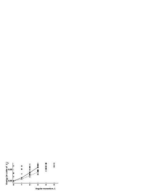
Figure 4: The energy spectra of a six-electron valley-unpolarized $\nu=1/3$-FQHE system shown for different Landau levels: $n=0$ (stars) and $n=1$ (dots). The flux quanta is $2S=15$. The spin-wave excitations are illustrated by solid ($n=1$) and dashed ($n=0$) lines.

The results shown in Fig. 3 correspond to the fully spin and valley polarized systems. This polarization is achieved at a high magnetic field due to the Zeeman splitting and the valley asymmetry. It is well known that even without the Zeeman energy the ground state of the non-relativistic system at $\nu=1/m$ is fully spin-polarizedfqhe_book ; fqhe_review with the spin equal to $S=N/2$, where $N$ is the number of particles. The situation is the same in graphene: the ground state of the $\nu=1/m$ liquid is fully spin and valley polarized. The results shown Fig. 3 describe the polarized excitations in such a system. Another type of neutral excitations of the incompressible liquid is the spin or pseudo-spin (valley) excitations. To explore these excitations we present the results of our calculations of the energy spectra for the $\nu=1/3$ ‘unpolarized’ system. Here we assume that the system is fully spin-polarized but valley-unpolarized. To characterize the states in such a system we consider the valley index as a pseudospin, $\tau$. Results of these calculations are shown in Fig. 4 for the zeroth and for the first Landau level. The ground state is at zero angular momentum and has a pseudospin equal to $\tau=N/2$, i.e. the pseudospin-polarized ground state. One type of excitations in a such system is the spin-waves. They are marked by the solid ($n=1$ Landau level) and dashed ($n=0$ Landau level) lines in Fig. 4. Another type of excitations corresponds to the energy branch formed by the lowest states at each angular momentum. The specific feature of these states is that the angular momentum of the state is related to the pseudospin value by the expression $(N/2)-\tau=L$. The physical meaning of these states is the Bose condensation of $L$ noninteracting pseudospin waveswojs . Clearly, in all the cases the energy scale at $n=1$ is larger than at $n=0$, which again illustrates the stronger interaction effects at $n=1$. However, this is not the general rule for the $n=1$ Landau level since we have seen from Fig. 2 that the pseudopotential at the zero relative momentum is stronger at the zeroth Landau level. This pseudopotential becomes important only for the unpolarized states when two electrons occupy the same spatial point, i.e. they have zero relative angular momentum. For those states the interaction effects can be stronger at the zeroth Landau level, as is the case of the $\nu=\frac{2}{3}$ incompressible stategr-fqhe . The excitation gap of the unpolarized $\nu=\frac{2}{3}$ state at the $n=0$ Landau level is larger than the excitation gap at the $n=1$ Landau levelgr-fqhe .

In the above calculations we have also included the valley asymmetry terms discussed in the previous section [see Eqs. (8)-(14)]. These corrections result into a very small shift of the energy levels up to magnetic field of 50 Tesla. Indeed, these terms are of the order of $a/l$. The magnetic length at $B=50$ T is about 3.6 nm, while the lattice constant of graphene is $a=0.246$ nm. The parameter $a/l$ is then really small ($\sim$0.07).

Finally, from the results presented above we conclude that the $1/m$-FQHE state in graphene is most stable at the $n=1$ Landau level. The inter-electron interaction effects are therefore more pronounced at the $n=1$ Landau levelgr-fqhe . This tendency is just the opposite to that of the non-relativistic system, where the excitation gap decreases monotonically with increasing Landau level index. The enhancement of the interaction effects at the higher Landau level index however depends on the filling factor.

II.2 Zero magnetic field

In the pseudospin space, the zero-magnetic-field Hamiltonian of a spin-up electron with a wavevector around the $K$ point iskane05 ; wang06 ; sini ${\cal H}=v\bm{p}\cdot\bm{\sigma}+\Delta_{\rm so}\sigma_{z}$ with $\bm{\sigma}=(\sigma_{x},\sigma_{y},\sigma_{z})$ the Pauli matrices and $\bm{p}$ the momentum operator. Here $\Delta_{\rm so}$ is the strength of the spin-orbit interaction (SOI). The eigenstates of the Schrödinger equation $H\Psi=E\Psi$ are readily obtained as $\Psi_{\bm{k}}^{\lambda}(\bm{r})=e^{i\bm{k}\cdot\bm{r}}{\small\left(\begin{array}[]{c}1+\sin(\alpha_{\bm{k}}+\lambda\pi/2)\\ -e^{i\phi_{\bm{k}}}\cos(\alpha_{\bm{k}}+\lambda\pi/2)\end{array}\right)}$ with energy $E_{\bm{k}}^{\lambda}=\lambda\sqrt{\Delta_{\rm so}^{2}+\hbar^{2}v^{2}k^{2}}$ for $\lambda=+1$ denoting the conduction band and $\lambda=-1$ the valance band. Here $\tan\phi_{k}=k_{y}/k_{x},\tan\alpha_{k}=\hbar vk/\Delta_{\rm so}$, and $k=\sqrt{k_{x}^{2}+k_{y}^{2}}$.

Figure 5: Diagrammatic illustration of the RPA dressed Coulomb interaction.

Using the techniques developed for the multicomponent systemsvint ; wang1 , it is straightforward to show that the RPA Coulomb interaction in the Fourier space $U(q,\omega)$ obeys the equation

$$U(q,\omega)=v_{0}+v_{0}\hat{\Pi}_{0}(q,\omega)U(q,\omega)$$ (15)

with the electron-hole propagator

$$\hat{\Pi}_{0}(q,\omega)=4\sum_{\lambda,\lambda^{\prime},\bm{k}}|g_{\bm{k}}^{\lambda,\lambda^{\prime}}(\bm{q})|^{2}\frac{f[E^{\lambda^{\prime}}_{\bm{k}+\bm{q}}]-f[E^{\lambda}_{\bm{k}}]}{\omega+E^{\lambda^{\prime}}_{\bm{k}+\bm{q}}-E^{\lambda}_{\bm{k}}+i\delta},$$ (16)

as illustrated by the Feymann diagram in Fig. 5. Here $v_{0}=e^{2}/(2\epsilon_{0}\epsilon_{i}q)$ is the two-dimensional Coulomb interaction (in Fourier space) with the high-frequency dielectric constantpere $\epsilon_{i}=1$ and $g_{\bm{k}}^{\lambda,\lambda^{\prime}}(\bm{q})$ is the interaction vertex.

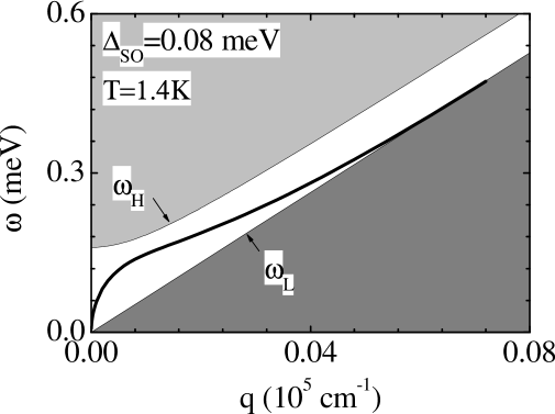
Figure 6: Plasmon spectrum (thick curves) of an electron gas in an intrinsic graphene ($E_{F}=0$) at temperatures $T=1.42$ K with $\Delta_{\rm so}=0.08$ meV. Intra- (dark shaded) and inter- (light shaded) band single-particle continuums are also shown. $\omega_{L}$ and $\omega_{H}$ are the lower and upper borders separating the white (EHC gap) and shaded areas respectively.

The factor four in Eq. (16) comes from the degenerate two spins and two valleys at $K$ and $K^{\prime}$; the vertex factor reads $|g^{\lambda,\lambda^{\prime}}_{\bm{k}}(\bm{q})|^{2}=[1+\lambda\lambda^{\prime}\cos\alpha_{\bm{k}+\bm{q}}\cos\alpha_{\bm{k}}+\lambda\lambda^{\prime}\sin\alpha_{\bm{k}+\bm{q}}\sin\alpha_{\bm{k}}(k+q\cos\theta)/|\bm{k}+\bm{q}|]/2$ with $\theta$ being the angle between $\bm{k}$ and $\bm{q}$. Since the chiral property of the system prohibits the intra-band backward scattering at $\bm{q}=2\bm{k}$ and the inter-band vertical transition at $\bm{q}=0$ under the Coulomb interaction in the system, we have $|g^{\lambda,-\lambda}_{\bm{k}}(0)|^{2}=|g^{\lambda,\lambda}_{\bm{k}}(2\bm{k})|^{2}=0$. The collective excitation spectrum is obtained by finding the zeros of the real part of the dielectric function $\hat{\epsilon}(q,\omega)=1-v_{0}(q)\hat{\Pi}_{0}(q,\omega)$.

In the presence of the SOI, an energy gap opens between the conduction and valence bands and the semimetal electronic system in graphene is converted into a narrow gap semiconductor system. At the same time, a gap is opened between its intraband single-particle continuum $\omega\leq\omega_{L}\equiv\hbar vq$ and its interband single-particle continuum $\omega\geq\omega_{H}\equiv 2\sqrt{\Delta_{\rm so}^{2}+\hbar^{2}v^{2}q^{2}/4}$. However, the system differs from a normal narrow gap semiconductor due to its peculiar chiral property. In this paper, we have chosen the magnitude of the SOI strength to be around $0.08-0.1$ meV in graphenekane05 ; mele . The result can be easily applied to Dirac gases with different $\Delta_{\rm so}$ by scaling the energy and wavevector in units of $\Delta_{\rm so}$ and $k_{\rm so}=\Delta_{\rm so}/(\hbar v)$ respectively.

Figure 7: Temperature dependence of the real part of the dielectric function at the edges of the intra- and intersubband single-particle continuum $\omega_{L}$ (dotted curve) and $\omega_{H}$ (solid curve) at $q=0.05\times 10^{5}$ cm^-1.

At zero temperature or for $T\ll\Delta_{\rm so}$, the intraband transition is negligible and $\epsilon_{r}>0$. There is no plasmon mode in the system. With an increase of the temperature, holes appear in the valence band and electrons in the conduction band. The intraband transitions are enhanced and contribute to the electron-hole propagator of Eq. (16) and a dip in $\epsilon_{r}$ at the intra-band EHC edge $\omega_{L}$. This dip in $\epsilon_{r}$ results in plasmon modes above $\omega_{L}$. For $\Delta_{\rm so}=0$ where $\omega_{H}=\omega_{L}$, the intraband (interband) single-particle continuum occupies the lower (upper) part of the $\omega-q$ space below $\omega_{L}$ (above $\omega_{L}$) and the plasmon mode are Landau damped. In the presence of the SOI, i.e. for $\Delta_{\rm so}\neq 0$, a gap of width $\omega_{H}-\omega_{L}$ is opened between the intra- and interband single-particle continuum and an undamped plasmon can exist in this gap as shown in Fig. 6. This plasmon mode may perhaps be observed in experiments.

The appearance of the undamped plasmon mode in the presence of the SOI is a result of the interplay between the intra- and the inter-band correlations which can be adjusted by varying the temperature of the system in experiments. To show the temperature range in which an undamped plasmon mode exists, in Fig. 7 we plot $\epsilon_{r}(\omega_{L})$ (dotted curve) and $\epsilon_{r}(\omega_{H})$ (solid curve) as functions of the temperature $T$ at $q=0.05\times 10^{5}$ cm^-1. For $\Delta_{\rm so}=0.08$ meV, an increase of the temperature from $T=0$ leads to an increase of the ratio of the intra- to the inter-band correlation while $\epsilon_{r}$ in the EHC gap ($\omega_{L}\leqslant\omega\leqslant\omega_{H}$) decreases and crosses zero. There is no undamped plasmon mode when the inter-band correlation dominates at $T\leq 1.1$ K and when the intra-band correlation dominates at $T\geq 3.3$ K. In the temperature regime 1.1 K $\leq T\leq 3.3$ K or $T\approx 2\Delta_{\rm so}$ when the intra- and inter-band correlations match, however, $\epsilon_{r}(\omega_{L})<0$ while $\epsilon_{r}(\omega_{H})>0$ and one undamped plasmon mode exists.

In summary: calculating the dynamic dielectric function taking into account the intrinsic spin-orbit interaction in graphene, we have studied the collective excitations in graphene. The Dirac electronic system in graphene is converted into a narrow gap semiconductor with chiral property by the spin-orbit interaction. As a result, an undamped collective excitation was found to exist in the spectral gap of the single-particle continuum and is perhaps observable in the experiments. More detailed results can be found elsewherewang06 . There have been a steady flow of reports in the literature on the electronic properties of graphene. Interestingly, our SOI-dependent dielectric function has recently been employed to explore the possibility of Wigner crystallization in graphenedaha .

References

References

- (1) K.S. Novoselov, et al., PNAS 102, 10451 (2005); Science 306, 666 (2004); Y. Zhang, et al., Phys. Rev. Lett. 94, 176803 (2005); C. Berger, et al., J. Phys. Chem. B 108, 19912 (2004).
- (2) P.R. Wallace, Phys. Rev. 71, 622 (1947).
- (3) T. Ando, in Nano-Physics & Bio-Electronics: A New Odyssey, edited by T. Chakraborty, F. Peeters, and U. Sivan (Elsevier, Amsterdam, 2002), Chap. 1.
- (4) J.W. McClure, Phys. Rev. 104, 666 (1956); R.R. Haering and P.R. Wallace, J. Phys. Chem. Solids 3, 253 (1957).
- (5) Y. Zheng and T. Ando, Phys. Rev. B 65, 245420 (2002).
- (6) K.S. Novoselov, et al., Nature 438, 197 (2005); Y. Zhang, Y.-W. Tan, H.L. Störmer, and P. Kim, ibid. 438, 201 (2005).
- (7) Y. Zhang, et al., Phys. Rev. Lett. 96, 136806 (2006).
- (8) V.P. Gusynin and S.G. Sharapov, Phys. Rev. Lett. 95, 146801 (2005); E. McCann and V.I. Fal’ko, ibid. 96, 086805 (2006).
- (9) M. Wilson, Phys. Today 59 (1), 21 (2006).
- (10) F.D.M. Haldane, Phys. Rev. Lett. 61, 2015 (1988).
- (11) C.L. Kane and E.J. Mele, Phys. Rev. Lett. 95, 226801 (2005).
- (12) X.F. Wang and T. Chakraborty, cond-mat/0605498.
- (13) N.A. Sinitsyn, et al., Phys. Rev. Lett. 97, 106804 (2006).
- (14) F.D.M. Haldane, Phys. Rev. Lett. 51, 605 (1983); F.D.M. Haldane and E.H. Rezayi, ibid. 54, 237 (1985).
- (15) K. Nomura and A.H. MacDonald, Phys. Rev. Lett. 96, 256602 (2006).
- (16) M.O. Goerbig, R. Moessner, and B. Doucot, cond-mat/0604554.
- (17) J. Alicea and M.P.A. Fisher, Phys. Rev. B 74, 075422 (2006).
- (18) G. Fano, F. Ortolani, and E. Colombo, Phys. Rev. B 34, 2670 (1986).
- (19) R.B. Laughlin, Phys. Rev. Lett. 50, 1395 (1983).
- (20) T. Chakraborty and P. Pietiläinen, The Quantum Hall Effects (Springer, Heidelberg, 1995), 2nd edition.
- (21) V.M. Apalkov and T. Chakraborty, Phys. Rev. Lett. 97, 126801 (2006).
- (22) T. Chakraborty, Adv. Phys. 49, 959 (2000).
- (23) A. Wojs and J.J. Quinn, Phys. Rev. B 66, 45323 (2002).
- (24) B. Vinter, Phys. Rev. B15, 3947 (1977).
- (25) X.F. Wang, Phys. Rev. B72, 85317 (2005).
- (26) N.M.R. Peres, F. Guinea, and A.H. Castro Neto, Phys. Rev. 72, 174406 (2005); J. Nilsson, A.H. Castro Neto, N.M.R. Peres, and F. Guinea, cond-mat/0512360 (2005).
- (27) D.P. DiVincenzo and E.J. Mele, Phys. Rev. B29, 1685 (1984).
- (28) H.P. Dahal, Y.N. Jogelkar, K.S. Bedell, and A.V. Balatsky, cond-mat/0609440 (2006).