Present address: ]Department of Physics, North Carolina State University, Raleigh, North Carolina 27695, USA

Theory of superconductivity of carbon nanotubes and graphene

Abstract

We present a new mechanism of carbon nanotube superconductivity that originates from edge states which are specific to graphene. Using on-site and boundary deformation potentials which do not cause bulk superconductivity, we obtain an appreciable transition temperature for the edge state. As a consequence, a metallic zigzag carbon nanotube having open boundaries can be regarded as a natural superconductor/normal metal/superconductor junction system, in which superconducting states are developed locally at both ends of the nanotube and a normal metal exists in the middle. In this case, a signal of the edge state superconductivity appears as the Josephson current which is sensitive to the length of a nanotube and the position of the Fermi energy. Such a dependence distinguishs edge state superconductivity from bulk superconductivity.

Superconductivity in carbon nanotubes (NTs) has been attracting much attention due to its high superconducting transition temperature, $T_{\rm c}\gtrsim 10$ K. tang01 ; takesue06 However, it is well-known that superconductivity in low dimensional (quasi-1D) systems is difficult to produce due to low density of states (DOS) saito98book , strong quantum fluctuations and other phenomena in such systems. Moreover, metallic NTs exhibit ballistic transport properties at low temperatures, bachtold00 which suggests a weak electron-phonon (el-ph) interaction for the conducting electrons. It is surprising that superconductivity is realized in NTs at such high values of $T_{\rm c}$. The mechanism of NT superconductivity is a critical issue and determining it will be a valuable contribution not only to NT science but also to nanotechnology.

Superconductivity has been observed in different types of NTs. Tang et al. reported $T_{\rm c}\sim 15$ K for single-wall NTs (SWNTs) having a diameter of 0.4 nm. tang01 Takesue et al. found an abrupt drop in the zero-bias resistance at 12 K for multi-wall NTs (MWNTs) having an outer diameter of $\sim$ 10 nm. takesue06 It is not straightforward to explain the results obtained in experiments. For instance, the DOS at the Fermi energy of a SWNT appears to be too small to give rise to such high $T_{\rm c}$. Kamide et al. kamide03 and Barnett et al. barnett05 considered that curvature of $(5,0)$ SWNTs may increase the DOS. However, a large DOS may induce charge density wave (CDW) before superconductivity occurs. Connétable et al. showed that $(5,0)$ and $(3,3)$ SWNTs undergo a CDW transition at temperatures above room temperature. connetable05 Thus, small diameter SWNTs may be insulators. Moreover the curvature effect is negligible for MWNTs. The origin of NTs superconductivity can not be explained by curvature-induced DOS and a new explanation is needed.

Here, we focus our attention on the large local DOS (LDOS) given by edge states which are intrinsic to graphene. The edge states are electronic localized states that exist around the zigzag edge of graphene and a SWNT. fujita96 ; nakada96 The energy dispersion of edge states is located near the Fermi energy ($E_{\rm F}=0$). The value of LDOS depends on the energy bandwidth ($W$) of the edge states. Recent experiments involving scanning tunneling microscopy/spectroscopy (STM/STS) at the zigzag edge of graphene, niimi05 ; kobayashi05 and angle-resolved photo-emission spectroscopy (ARPES) of Kish graphite, sugawara06 showed that the edge states are located below the Fermi energy and have a finite $W$. Although edge states of NTs have not been observed so far, it is possible to consider the edge states of a SWNT with a zigzag edge as well as those of a graphene sheet.

In this letter, we calculate $T_{\rm c}$ as a function of $W$ and $E_{\rm F}$, and obtain an appreciable values for $T_{\rm c}$ of the edge states of zigzag SWNTs and graphene. As a result, we predict that the superconductivity of a SWNT is given by a natural superconductor/normal metal/superconductor junction (SNS) system, in which superconducting states develop locally at both ends of the SWNT and a normal, ballistic state exists in the middle of the SWNT. Remarkably, the bulk part of a SWNT need not be superconducting since Josephson supercurrent flows in the middle as a result of the proximity effect when the superconducting edge states have different phases at both ends. We note that proximity-induced supercurrents have been observed in Ta/SWNTs/Au kasumov99 and Nb/MWNTs/Al systems. haruyama04 The Josephson current of a metallic zigzag SWNT depends on the length ($L$) and temperature ($T$). The amplitude of the current is proportional to $\exp(-L/\xi_{N})$ when $T<T_{0}$ where $T_{0}\sim 20\mu{\rm m}/L$ K and $\xi_{N}\sim 10^{3}{\rm K}/T$ nm is the coherence length, wakabayashi02 which is a characteristic feature of conventional SNS transport theory for the clean limit. kulik70 A length dependence of the current distinguishes edge-state superconductivity from bulk superconductivity.

The edge-state superconductivity has the following advantages in explaining the experiment performed by Takesue et al., takesue06 (1) the edge states are robust against static surface deformation which is relevant for CDW instability, fujita97 ; sasaki06jpsj (2) the el-ph interaction for the edge states is strong compared with that for delocalized states, and (3) $T_{\rm c}$ is sensitive to $W$ and the energy position of $E_{\rm F}$, which are all consistent with the fact that the superconductivity is sensitive to the junction structures of the Au electrode/MWNTs. takesue06 Enhancement of $T_{\rm c}$ at the edge is important for understanding superconductivity of a general surface state, not only for graphite materials but also for noble-metals such as gold. kevan87

The edge states are zero-energy ($E(k)=0$) eigenstates of the nearest-neighbor (nn) tight-binding Hamiltonian, ${\cal H}_{\rm nn}|\Psi(k)\rangle=E(k)|\Psi(k)\rangle$. fujita96 ; sasaki05prb ; sasaki06apl $k\equiv{\bf k}\cdot{\bf a}_{1}$ is the wavevector around the tube axis where ${\bf a}_{1}$ is the unit vector along the edge (see Fig. 1(a)). The edge states exist for $2\pi/3<k<4\pi/3$. The wavefunction is written as

$$|\Psi(k)\rangle=\sum_{i\in{\rm A}}C_{i}(k)|\phi({\bf R}_{i})\rangle,$$ (1)

where $|\phi({\bf R}_{i})\rangle$ is the 2${\rm p}_{z}$ orbital, and $C_{i}(k)$ is the amplitude at ${\bf R}_{i}$ and has a value on one of the two sublattices (A and B) of graphite. fujita96 In the direction of the SWNT axis, the magnitude of $C_{i}(k)$ quickly decays from the edge to the interior region. The localization length is given by $\xi(k)=-|{\bf T}|/2\ln|2\cos(k/2)|$ ($2\pi/3<k<4\pi/3$) where ${\bf T}=2{\bf a}_{2}-{\bf a}_{1}$ is the translation vector. sasaki06apl ; sasaki05prb When we incorporate the next nearest-neighbor (nnn) transfer integral $\gamma_{n}$ into the Hamiltonian, the energy dispersion of the edge states becomes $E(k)=\gamma_{n}(2\cos k+1)$ ($2\pi/3<k<4\pi/3$) where the value of $\gamma_{n}=0.3$ eV is adopted. sasaki06apl ; porezag95 The calculated results explain the STS niimi05 ; kobayashi05 and ARPES sugawara06 experiments. Hereafter we treat $W$ ($=\gamma_{n}$) and the position of the Fermi energy as independent parameters.

The el-ph interaction for the edge states shows a different behavior from that for delocalized states. The el-ph interaction consists of on-site and off-site deformation potentials. jiang05 It is pointed out that, for a backward scattering of delocalized states, the on-site deformation potentials on two sublattices cancel with each other due to a phase difference of the wavefunction at the two sublattices. suzuura02 This is a reason why metallic NTs show a ballistic transport property. However, the cancellation of the on-site deformation potential does not work for the edge states since the wavefunction of the edge state has an amplitude only on one of the two sublattices. Furthermore, because of a lack of translational symmetry at the edge, a strong el-ph interaction for optical phonon modes is expected for the edge. Thus the understanding of the el-ph interaction for the edge states is essential for the present problem.

The el-ph Hamiltonian is defined by ${\cal H}={\cal H}_{0}+{\cal H}_{\rm int}$, where ${\cal H}_{0}$ represents the edge states and phonon, and ${\cal H}_{\rm int}$ is the el-ph interaction. ${\cal H}_{0}$ is given by $\sum_{k}E(k)c_{k}^{\dagger}c_{k}+\sum_{{\bf q},\nu}\omega_{\nu}({\bf q})b_{{\bf q},\nu}^{\dagger}b_{{\bf q},\nu}$, where $c_{k}$ is the annihilation operator of edge state and $b_{{\bf q},\nu}$ is the annihilation operator of $\nu$-th phonon mode with momentum ${\bf q}$ and energy $\omega_{\nu}({\bf q})$. For a graphite unit cell, there are six phonon eigen-modes; out-of-plane tangential acoustic/optical mode (oTA/oTO), in-plane tangential acoustic/optical mode (iTA/iTO), and longitudinal acoustic/optical mode (LA/LO). $\omega_{\nu}({\bf q})$ and phonon eigenvector are obtained by solving a $6\times 6$ dynamical matrix. jiang05 The el-ph interaction is given by

$${\cal H}_{\rm int}=\frac{1}{\sqrt{N_{\rm u}}}\sum_{k,k^{\prime}}\sum_{q_{t},\nu}\alpha^{\nu}_{kk^{\prime}}({\bf q})(b_{{\bf q},\nu}+b_{{\bf-q},\nu}^{\dagger})c_{k^{\prime}}^{\dagger}c_{k},$$ (2)

where $N_{\rm u}$ is the number of graphite unit cells in a SWNT, and $\alpha^{\nu}_{kk^{\prime}}({\bf q})$ is the el-ph coupling connecting two edge states $k$ and $k^{\prime}$ by $\nu$-th phonon mode with momentum ${\bf q}$. Due to the momentum conservation along the edge, $k^{\prime}=k+q$ ($q\equiv{\bf q}\cdot{\bf a}_{1}$), while the wavevector perpendicular to the edge $q_{t}$ ($\equiv{\bf q}\cdot{\bf T}$) is needed to sum over the Brillouin zone.

We calculate $\alpha^{\nu}_{kk^{\prime}}({\bf q})$ using the deformation potential, $\delta V=-\sum_{p}\nabla v({\bf R}_{p})\cdot{\bf u}({\bf R}_{p})$, where ${\bf u}({\bf R}_{p})$ is the displacement vector and $v({\bf R}_{p})$ is the pseudo-potential of a carbon atom at ${\bf R}_{p}$. The present pseudo-potential is used for calculating resonance Raman intensity in which the calculated results explain chirality and diameter dependence of Raman intensity quantitatively. jiang05 ${\bf u}({\bf R}_{p})$ can be expanded by phonon normal modes as ${\bf u}({\bf R}_{p})=\sum_{{\bf q},\nu}(A^{\nu}({\bf q})/\sqrt{2N_{\rm u}})(b_{{\bf q},\nu}+b_{{\bf-q},\nu}^{\dagger}){\bf e}^{\nu}_{\bf q}({\bf R}_{p})e^{i{\bf q}\cdot{\bf R}_{p}}$, where ${\bf e}^{\nu}_{\bf q}({\bf R}_{p})$ is the normalized eigenvector at ${\bf R}_{p}$ and $A^{\nu}({\bf q})=\hbar/\sqrt{m_{c}\omega_{\nu}({\bf q})}$ is the phonon amplitude. From $\langle\Psi(k^{\prime})|\delta V|\Psi(k)\rangle$, we obtain $\alpha^{\nu}_{kk^{\prime}}({\bf q})\equiv A^{\nu}({\bf q})M^{\nu}_{kk^{\prime}}({\bf q})/\sqrt{2}$, where $M^{\nu}_{kk^{\prime}}({\bf q})$ is the el-ph matrix element defined by

$$M^{\nu}_{kk^{\prime}}({\bf q})\equiv-\sum_{p>0}\langle\Psi(k^{\prime})|\nabla v({\bf R}_{p})|\Psi(k)\rangle\cdot{\bf e}^{\nu}_{\bf q}({\bf R}_{p})e^{i{\bf q}\cdot{\bf R}_{p}}.$$ (3)

Putting Eq. (1) to Eq. (3), we see that $M^{\nu}_{kk^{\prime}}({\bf q})$ consists of the on-site $\langle\phi({\bf R}_{i})|\nabla v({\bf R}_{p})|\phi({\bf R}_{i})\rangle$ and off-site $\langle\phi({\bf R}_{p})|\nabla v({\bf R}_{p})|\phi({\bf R}_{i})\rangle$ atomic deformation potentials (${\bf R}_{p}\neq{\bf R}_{i}$). The off-site atomic deformation potential does not contribute to $M^{\nu}_{kk^{\prime}}({\bf q})$ because $\langle\phi({\bf R}_{p})|\nabla v({\bf R}_{p})|\phi({\bf R}_{i})\rangle$ vanishes for $|{\bf R}_{p\in A}-{\bf R}_{i}|\gtrsim|{\bf a}_{1}|$. jiang05 We note that Eq. (3) includes the effect of boundary. To show this, we illustrate several carbon atoms (${\bf R}_{p>0}$) near the zigzag edge and a fictitious atom (${\bf R}_{p<0}$) in Fig. 1(a). The on-site deformation potential at ${\bf R}_{1}$ is given mainly by the vibrations of carbon atoms at ${\bf R}_{2}$ and ${\bf R}_{3}$ as $-\sum_{p=2,3}\langle\phi({\bf R}_{1})|\nabla v({\bf R}_{p})|\phi({\bf R}_{1})\rangle\cdot{\bf e}^{\nu}_{\bf q}({\bf R}_{p})e^{i{\bf q}\cdot{\bf R}_{p}}$. This on-site deformation potential would be canceled by the fictitious carbon atom at ${\bf R}_{-1}$ since ${\bf e}^{\nu}_{\bf q}({\bf R}_{p})$ ($p=-1,2,3$) points at the same direction. Namely, the on-site deformation potential is enhanced at the edge. This enhancement may be a reason why the tunnel current is unstable at the edge. niimi05

For a $(n,0)$ SWNT, $k$ for the edge states becomes discrete as $k(i)=2\pi/3+2\pi i/n$ ($i=1,\ldots,n/3-1$) due to the periodic boundary condition around the axis. We denote an edge state by the integer $i$ and write $M^{\nu}_{k(i)k(j)}({\bf q})$ as $M^{\nu}_{ij}({\bf q})$ for simplicity. Putting $k(i)$ to $\xi(k)$, we obtain $\xi(k)\lesssim d_{t}/2$ where $d_{t}\equiv n|{\bf a}_{1}|/\pi$ is diameter for the SWNT.

In Fig. 1(b) and (c), we plot $|M^{\nu}_{14}({\bf q})|$ and $|M^{\nu}_{69}({\bf q})|$, respectively, for the $(60,0)$ SWNT ($d_{t}\approx 5$ nm). $|M_{14}^{\nu}({\bf q})|$ is chosen as an example that $\xi(1)\sim$ 22Å and $\xi(4)\sim$ 4.4Å are much longer than the carbon-carbon bond length $a_{\rm cc}\sim$ 1.4Å, while $|M_{69}^{\nu}({\bf q})|$ is chosen as another example that $\xi(6)\sim 2.4$Å and $\xi(9)\sim 0.9$Å are comparable to $a_{\rm cc}$. As for acoustic modes, the LA mode couples strongly to the edge state. The oTA mode contributes to $|M^{\nu}_{14}({\bf q})|$, whereas the iTA mode is negligible. Since the LA and oTA modes change the area of a hexagonal lattice, they contribute to on-site deformation potential. For optical modes, the iTO and LO modes are important. $|M_{14}^{\rm iTO}({\bf q})|$ decreases with increasing $q_{t}$, while $|M_{14}^{\rm LO}({\bf q})|$ increases with increasing $q_{t}$. As shown in Fig. 1(c), the deformation potential is stronger for the smaller localization length. The behavior of the iTO and LO modes is due to the boundary deformation potential. To prove this, we show in the inset, the matrix element without the boundary, which is defined by Eq. (3) including (fictitious) carbon atoms at $p<0$ in Fig. 1(a). The boundary deformation potential depends on the direction of ${\bf e}_{\bf q}^{\nu}$ and the magnitude is maximum when ${\bf e}_{\bf q}^{\nu}$ is parallel to ${\bf T}$. ${\bf e}_{\bf q}^{\rm iTO}$ (${\bf e}_{\bf q}^{\rm LO}$) has a large element parallel to ${\bf T}$ when $q_{t}<\sqrt{3}q$ ($q_{t}>\sqrt{3}q$) as shown as a vertical line in Fig. 1(b) and (c). On the other hand, ${\bf e}_{\bf q}^{\rm oTO}$ is perpendicular to the SWNT axis (or parallel to ${\bf a}_{1}\times{\bf T}$) and the boundary effect of the oTO mode does not appear in $|M_{ij}^{\rm oTO}({\bf q})|$.

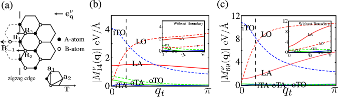
Figure 1: (Color online) (a) Carbon atoms at ${\bf R}_{p>0}$ near the zigzag edge, and a fictitious carbon atom at ${\bf R}_{-1}$ are illustrated to show an enhancement of the on-site deformation potential at the boundary. The boundary deformation potential is large for optical modes whose ${\bf e}_{\bf q}^{\nu}$ is parallel to ${\bf T}$. (b,c) $|M_{ij}^{\nu}({\bf q})|$ of the $(60,0)$ SWNT with (b) $k(1)(=7\pi/10)\to k(4)(=4\pi/5)$ and (c) $k(6)(=13\pi/15)\to k(9)(=29\pi/30)$ are plotted as a function of $q_{t}$ where $q=\pi/10$. The inset is the matrix element including (fictitious) carbon atoms at ${\bf R}_{p<0}$. Three solid/dashed curves represent acoustic/optical phonon modes: oTA/oTO(green), iTA/iTO(blue) and LA/LO (red). The vertical dashed lines represent $q_{t}=\sqrt{3}q$ ($\sqrt{3}=|{\bf T}|/|{\bf a}_{1}|$).

Now we apply $|\alpha_{kk^{\prime}}^{\nu}({\bf q})|$ to the Eliashberg equation. The Eliashberg equation includes the effects of phonon retardation and electron self-energy, which are not taken into account in the BCS theory. eliashberg60 ; nambu60 The phonon retardation is included by the Matsubara frequency: $\omega_{n}=k_{\rm B}T(2n+1)\pi$ where $n$ is integer and $|\omega_{n}|\leq\omega_{\rm D}$ where $\omega_{\rm D}=0.2$ eV is the Debye energy. saito98book Since the gap function, $\Delta(k,i\omega_{n})$, vanishes at $T_{\rm c}$, the Eliashberg equation can be linearized at $T_{\rm c}$ to get the gap equation:

$$\Delta(k,i\omega_{n}) =\frac{2k_{\rm B}T_{\rm c}}{N_{\rm u}}\sum_{k^{\prime},m,q_{t},\nu}\frac{|\alpha^{\nu}_{kk^{\prime}}({\bf q})|^{2}\omega_{\nu}({\bf q})}{(\omega_{n}-\omega_{m})^{2}+\omega_{\nu}^{2}({\bf q})}$$

$$\times|G(k^{\prime},i\omega_{m})|^{2}\Delta(k^{\prime},i\omega_{m}),$$ (4)

where $G(k,i\omega_{n})$ is a thermal Green function of electron, $G(k,i\omega_{n})=(i\omega_{n}-(E(k)-E_{\rm F})-\Sigma(k,i\omega_{n}))^{-1}$. Here, $\Sigma(k,i\omega_{n})$ is the self-energy, which is determined self-consistently by

$$\Sigma(k,i\omega_{n})=\frac{2k_{\rm B}T_{\rm c}}{N_{\rm u}}\sum_{k^{\prime},m,q_{t},\nu}\frac{|\alpha^{\nu}_{kk^{\prime}}({\bf q})|^{2}\omega_{\nu}({\bf q})}{(\omega_{n}-\omega_{m})^{2}+\omega_{\nu}^{2}({\bf q})}G(k^{\prime},i\omega_{m}).$$ (5)

After calculating $\Sigma(k,i\omega_{n})$ in Eq. (5), we solve Eq. (4).

In Fig. 2, we show $T_{\rm c}$ as a function of $W$ for $(n,0)$ SWNTs with $n=30,60,$ and 90, where we assume $E_{\rm F}=-W/2$. $T_{\rm c}$ decreases with increasing $W$ and $T_{\rm c}$ vanishes at critical values, $W_{\rm c}$. The increase of $W$ corresponds to the decrease of the LDOS around the Fermi energy. The values of $W_{\rm c}$ are 0.46 eV and 0.37 eV, respectively for $n=30$ and $n\geq 60$. Those values of $W_{\rm c}$ are close to $\gamma_{n}$ (the dashed line in Fig. 2). When $n$ ($d_{t}$) is relatively small, all edge states couple strongly to the boundary deformation potential since ${\rm max}(\xi)\lesssim d_{t}/2$. The strong el-ph coupling for $n=30$ makes $W_{\rm c}$ larger than that for $n\geq 60$. It is also noted that excluding optical modes makes $T_{\rm c}$ and $W_{\rm c}$ both smaller. In this case, we obtain $T_{\rm c}\sim$ 70 K at $W=0$ eV and $W_{\rm c}\sim$ 0.21 eV for $n=60$. Although the values of $A^{\nu}({\bf q})$ for optical modes are smaller than those of acoustic modes, the iTO and LO modes contribute to Eqs. (4) and (5) because of the large values of $|M_{ij}^{\nu}({\bf q})|$ due to the boundary deformation potential. A large value of $n$ corresponds to the zigzag edge of graphene. Remarkably, $T_{\rm c}$ for $n=120$ has a curve quite similar to $T_{\rm c}$ for $n=90$. This suggests that $T_{\rm c}$ converges and $n=90$ is large enough to represent a graphene.

Figure 2: The dependence of $T_{\rm c}$ on $W$ is plotted for $(30,0)$, $(60,0)$ and $(90,0)$ zigzag SWNTs. The Fermi energy is assumed to be located at the center of the band ($E_{\rm F}=-W/2$). The nnn hopping gives $W=0.3$ eV. (inset) The dependence of $T_{\rm c}$ on $E_{\rm F}$ for the $(60,0)$ SWNT with $W=\gamma_{n}$.

It is important to note that the calculated $T_{\rm c}$ is sensitive to the energy position of $E_{\rm F}$. We plot $T_{\rm c}$ as a function of $E_{\rm F}$ for a $(60,0)$ SWNT with $W=\gamma_{n}$ in the inset of Fig. 2. When $E_{\rm F}$ exists at the top of the energy band of the edge states, $T_{\rm c}$ becomes less than 1 K. When $E_{\rm F}\sim-0.1$ eV, $T_{\rm c}$ decreases rapidly since the inelastic scattering process is suppressed by the absence of the scattered state. This is a reason why $T_{\rm c}$ is sensitive to the position of $E_{\rm F}$. We also calculated $T_{\rm c}$ for extended states around the Fermi energy of the $(60,0)$ SWNT using the Eliashberg equation. The calculated $T_{\rm c}$ is less than 0.1 K. Thus the extended states do not contribute to $T_{\rm c}$.

The observed $T_{\rm c}$ should be smaller than our estimation. In fact, a lattice defect along the edge decreases LDOS and reduces $T_{\rm c}$. The Coulomb repulsive interaction might decrease $T_{\rm c}$, too. Fujita et al. showed that the edge states develop a local ferro-magnetism in the presence of a large Hubbard $U$ comparable to $W$. fujita96 Since the edge states are localized at the edge, they might have a quantum fluctuation intrinsic to 1D system. The Tomonaga-Luttinger liquid theory may be suitable to calculate the correlation function.

In summary, using the Eliashberg equation, we clarify that $W$ and $E_{\rm F}$ position is sensitive to $T_{\rm c}$ of the edge states in SWNTs and graphene. The rather high value of $T_{\rm c}$ obtained is a result of LDOS enhancement by the edge states, and the on-site and boundary deformation potentials of the el-ph interaction for the edge states. If nanotube superconductivity is given by el-ph interaction, the edge-state superconductivity is a unique candidate since $T_{\rm c}$ of the bulk is negligible. Edge (surface) state superconductivity is potentially a key concept for designing superconductors on the nanometer scale.

R. S. acknowledges a Grant-in-Aid (No. 16076201) from MEXT.

References

- (1) Z. K. Tang et al., Science 292, 2462 (2001).
- (2) I. Takesue et al., Phys. Rev. Lett. 96, 57001 (2006).
- (3) R. Saito, G. Dresselhaus, and M. Dresselhaus, Physical Properties of Carbon Nanotubes (Imperial College Press, London, 1998).
- (4) A. Bachtold et al., Phys. Rev. Lett. 84, 6082 (2000).
- (5) K. Kamide, T. Kimura, M. Nishida, and S. Kurihara, Phys. Rev. B 68, 24506 (2003).
- (6) R. Barnett, E. Demler, and E. Kaxiras, Phys. Rev. B 71, 35429 (2005).
- (7) D. Connétable, G. M. Rignanese, J. C. Charlier, and X. Blase, Phys. Rev. Lett. 94, 15503 (2005).
- (8) M. Fujita, K. Wakabayashi, K. Nakada, and K. Kusakabe, J. Phys. Soc. Jpn. 65, 1920 (1996).
- (9) K. Nakada, M. Fujita, G. Dresselhaus, and M. S. Dresselhaus, Phys. Rev. B 54, 17954 (1996).
- (10) Y. Niimi et al., Appl. Surf. Sci. 241, 43 (2005).
- (11) Y. Kobayashi et al., Phys. Rev. B 71, 193406 (2005).
- (12) K. Sugawara et al., Phys. Rev. B 73, 45124 (2006).
- (13) A. Y. Kasumov et al., Science 284, 1508 (1999).
- (14) J. Haruyama et al., Appl. Phys. Lett. 84, 4714 (2004).
- (15) K. Wakabayashi, J. Phys. Soc. Jpn. 72, 1010 (2002).
- (16) I. O. Kulik, Sov. Phys. JETP 30, 944 (1970).
- (17) M. Fujita, M. Igami, and K. Nakada, J. Phys. Soc. Jpn. 66, 1864 (1997).
- (18) K. Sasaki, S. Murakami, and R. Saito, J. Phys. Soc. Jpn. 75, 074713 (2006).
- (19) S. D. Kevan and R. H. Gaylord, Phys. Rev. B 36, 5809 (1987).
- (20) K. Sasaki, S. Murakami, and R. Saito, Appl. Phys. Lett. 88, 113110 (2006).
- (21) K. Sasaki, S. Murakami, R. Saito, and Y. Kawazoe, Phys. Rev. B 71, 195401 (2005).
- (22) D. Porezag et al., Phys. Rev. B 51, 12947 (1995).
- (23) J. Jiang et al., Phys. Rev. B 72, 235408 (2005).
- (24) H. Suzuura and T. Ando, Phys. Rev. B 65, 235412 (2002).
- (25) G. M. Eliashberg, Sov. Phys. JETP 11, 696 (1960).
- (26) Y. Nambu, Phys. Rev. 117, 648 (1960).