Simulations of some quantum gates, with decoherence

Abstract

Methods and results for numerical simulations of one and two interacting rf-SQUID systems suitable for adiabatic quantum gates are presented. These are based on high accuracy numerical solutions to the static and time dependent Schroedinger equation for the full SQUID Hamiltonian in one and two variables. Among the points examined in the static analysis is the range of validity of the effective two-state or “spin 1/2” picture. A range of parameters is determined where the picture holds to good accuracy as the energy levels undergo gate manipulations. Some general points are presented concerning the relations between device parameters and “good” quantum mechanical state spaces.

The time dependent simulations allow the examination of suitable conditions for adiabatic behavior, and permits the introduction of a random noise to simulate the effects of decoherence. A formula is derived and tested relating the random noise to the decoherence rate. Sensitivity to device and operating parameters for the logical gates NOT and CNOT are examined, with particular attention to values of the tunnel parameter $\beta$ slightly above one. It appears that with values of $\beta$ close to one, a quantum CNOT gate is possible even with rather short decoherence times.

Many of the methods and results will apply to coupled double-potential well systems in general.

I Introduction

In previous work we have described quantum logic gates based on the rf SQUID. The basic operation involved is an adiabatic inversion, where the SQUID reverses flux states under the sweep of an external field $\phi^{ext}$. This is equivalent to the logical NOT deco . When a second SQUID is added whose flux can add or subtract from $\phi^{ext}$, parameter ranges were found for the two $\phi_{1}^{ext},\phi_{2}^{ext}$ so that the two-SQUID system undergoes a reshuffling of levels equivalent to the logical operation CNOT ref1 ,pla .

In this paper we present a study of these systems by numerical simulations which enable us to examine these processes in more quantitative detail. Among the points we can examine is the validity of the “spin 1/2 picture”. In the previous work we often found good agreement with a simplified “spin 1/2 analogy” where the two lowest states of each SQUID are treated as an effective two-state system. This picture is very useful in understanding and predicting the behavior of the systems and here we examine its validity by simulations for the full many-state system.

A further question which can be studied in detail is adiabaticity. This is the operating principle for our quantum gates and it is necessary to know under which conditions it holds.

Finally, we can use our programs to study the effects of decoherence on the quantum gates. We will examine how to introduce decoherence as a noise signal and study its effects on our operations.

It should be stressed that our results would have been difficult if not impossible to obtain without the extensive system of numerical programs. Due to the sensitivity to the various parameters and the subtleties of the tunneling problem, analytic methods would be difficult and uncertain. With the high accuracy programs, a short run can replaces otherwise long, complicated, and often approximate formulas.

II One variable System

We begin by shortly reviewing our approach  ref1 , pla as applied to the one variable, one rf SQUID system, at first without decoherence. This will allow us to fix the notation and parameters, and to establish the connection between the full Hamiltonian and the “spin 1/2 picture”.

II.1 Squid Hamiltonian

The SQUID Hamiltonian in terms of the capacitance $C$ and inductance $L$ of the junction is ${\cal H}={-1\over 2C({\Phi_{0}\over 2\pi})^{2}}{\partial^{2}\over\partial\phi^{2}}+U$ with $U=({\Phi_{0}\over 2\pi})^{2}{1\over L}\{{1\over 2}[(\phi-\phi^{ext})^{2}]+\beta cos\phi\}$, where $\beta=\frac{2\pi LI_{c}}{\Phi_{0}}$, $I_{c}$ being the critical current for the junction rev . The variable $\phi$ is the flux $\Phi$ in the SQUID loop in flux quantum units $\phi=\Phi{2\pi\over\Phi_{0}}$, and furthermore shifted by $\pi$ so that $\phi=0$ corresponds to the maximum at the center of the double potential well $U$. Similarly $\phi^{ext}$ is an external field, where due to the shift, $\phi^{ext}=0$ corresponds to a non-zero applied field of size $\frac{\Phi_{0}}{2}$. By factoring out an overall energy scale $E_{0}=1/\sqrt{LC}$ so that ${\cal H}=E_{0}H$ we obtain the dimensionless hamiltonian

$$H={-1\over 2\mu}{\partial^{2}\over\partial\phi^{2}}+V_{0}\{{\textstyle\frac{1}{2}}[(\phi-\phi^{ext})^{2}]+\beta\,cos\phi\}={-1\over 2\xi}{\partial^{2}\over\partial\phi^{2}}+\xi\{{\textstyle\frac{1}{2}}[(\phi-\phi^{ext})^{2}]+\beta\,cos\phi\}\;.$$ (1)

With this choice of the factor $E_{0}$ the “mass” $\mu$ and the “potential” $V_{0}$ are equal, hence the second form in terms of a common parameter $\xi$, whose value is $\xi=\mu=V_{0}\approx 1030\sqrt{{C/pF\over L/pH}}$. In effect the capacitance C and inductance L have been exchanged for an energy scale $E_{0}$ and a dimensionless number $\xi$. We shall discuss the physical meaning of $\xi$ below.

In the following we shall endeavor to express all energies in terms of the general energy unit $E_{0}$ and all times in the time unit $1/E_{0}$. To converted these to dimensional units one multiplies by $E_{0}=6.4\times 10^{-4}eV\times(L/pH~{}C/pF)^{-1/2}=1.0\times 10^{12}~{}radians/sec~{}\times(L/pH~{}C/pF)^{-1/2}=7.7K\times(L/pH~{}C/pF)^{-1/2}$ and for the time by $1/E_{0}=1.0\times 10^{-12}seconds\times(L/pH~{}C/pF)^{1/2}$  correct . Thus results with the dimensionless Hamiltonian, Eq 1, which we will use in our computer simulations, are to be converted to physical energies by multiplying by $E_{0}$. Typical values $L=400pH$ and $C=0.1pF$ for example, yield $E_{0}=160\times 10^{9}radians/sec=1.2\,K$ and $\xi=16.3$, while the time unit is $6.3\times 10^{-12}~{}sec$. We will use these values for “typical examples” or when absolute times or energies are needed. We shall usually work with $\beta=1.19$, which for $L=400pH$ corresponds to a critical current of about $1\,\mu A$.

To carry out calculations with Eq 1 for the eigenvalues and eigenfunctions, the numerical method employed a large basis of harmonic oscillator wavefunctions and expanded the cosine as a low order polynomial. Since in the harmonic oscillator basis polynomials are simple, sparse, matrices, the problem is reduced to algebraic manipulations and a matrix diagonalization. It was usually found that an expansion up to 8th order for the cosine and a basis of 256 oscillator states gave numerical stability. A typical run with a few hundred basis vectors on a Pentium 4 machine lasts less than a minute and resolves our smallest energy splitting to better than two significant figures.

II.2 Parameters of the Hamiltonian

Eq 1 contains three parameters, $\phi^{ext}$, $\beta$ and $\xi$. The applied flux $\phi^{ext}$  controls the asymmetry of the potential and for $\phi^{ext}$=0 the potential is symmetric. Fig. 1, Left, shows an example with the potential in this symmetric configuration. In this “level crossing” situation the energy splitting of the lowest pair of levels is just the tunneling energy $\omega_{tunnel}$ and so is quite small. Here it is 0.0044 and not clearly resolved on the plot.

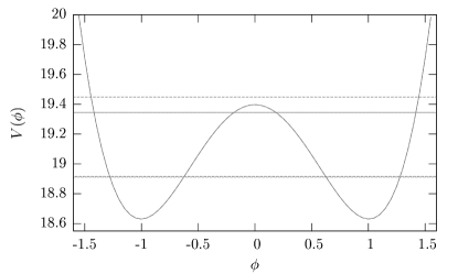
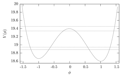
Figure 1: Potential with first four energy levels according to Eq 1, for $\beta=1.19$ and $V_{0}=\mu=16.3$. Left: The symmetric or “level crossing” configuration with $\phi^{ext}$=0. The lowest line represents a pair of levels which are not clearly resolved on the plot. Right: An asymmetric configuration with $\phi^{ext}$=0.0020, showing a much greater pair separation. The horizontal axis represents the reduced flux $\phi$, the vertical axis the energy in units of $6.4\times 10^{-4}eV(L/pH~{}C/pF)^{-1/2}$.

Fig. 1, Right, shows, under the same conditions, an asymmetric configuration with $\phi^{ext}$=0.0020. To produce an adiabatic inversion or NOT, $\phi^{ext}$ begins at such a non-zero value and adiabatically ”sweeps” to the opposite value. The level splitting is now dominated by the shift of the potential and not the tunneling. The splitting of the lowest pair is 0.060, an order of magnitude greater than in the symmetric configuration. The wavefunctions of the energy eigenstates are now concentrated in the left or right well, while at “level crossing” they were $\pm$ linear combinations of these states.

Turning to the parameter $\xi$, raising its value both increases the ”mass” and the height of the potential and so will generally lead to a greater concentration of the wavefunction in one of the potential wells, as well as a reduction of the tunneling. In the wells one has roughly harmonic oscillator potentials, for which the ground state wavefunction is $\psi\sim e^{-{1\over 2}\sqrt{c\mu V_{0}}\phi^{\prime 2}}$, where $\phi^{\prime}$ means $\phi$ referred to its equilibrium position and $c$ is a factor of order one. Thus $\xi$ gives the spread of the wavefunction in the well; it controls how “uncertain” the flux is when it is in a “definite” state. Similarly the exponent in the tunneling factor $e^{-\int dx\sqrt{2\mu(V_{0}-E)}}$ increases with $\xi$ and reduces the tunneling. Therefore $\xi=\sqrt{\mu V_{0}}$ may be viewed as a measure of how ”classical” the wavefunction is, and the relatively large value of $\xi$ we deal with indicates that our component wavefunctions are rather well defined and ”classical” in this sense. That is although we deal with linear combinations of states, these basis states themselves are relatively localized, are rather “classical”. Examples of this will be presented in Fig. 9.

The parameter $\beta$, finally, has a strong effect on the tunneling since increasing its value both widens and heightens the barrier. Thus increasing $\beta$ from 1.19 to 1.35 leads to three pairs of well defined states below the barrier, with a tunnel splitting of only $2.0\times 10^{-6}$ for the lowest pair. In the other direction, for $\beta$ somewhat less than one, there are no longer any states localized around a definite value of the flux at all. The most interesting region for the present purposes appears to be the values of $\beta$ somewhat greater than one, and for most of our simulations we shall use $\beta=1.19$. With $\beta=1.19,\xi=16.3$, the splitting at level crossing is 0.0044, while the distance to the next set of levels is 0.48. This difference of two orders of magnitude provides a factor of ten margin in manipulating the levels with still a factor of ten to the next set. However in studying specific designs it may be of interest to make a careful study of the behavior with respect to $\beta$ in the vicinity of one, and we shall also briefly consider $\beta=1.14$.

Finally, it should be observed that the energy splitting from our lowest pair of states to the next ones is on the order of the energy unit, which is $E_{0}\sim 1\,K$. Consequently when working well below $1K$, which we shall assume, one can expect only the lowest pair of states to be populated, and the neglect of thermal over-the-barrier transitions to be justified.

III Identification with a Spin 1/2 System

It is frequently a useful simplification to use the “spin picture” where we treat two closely separated levels, such as the lowest pair in Fig. 1, as the two states of a “spin 1/2 system” us ; and for the two qubit system as two such spins. In this section we discuss the relation between this picture and the full Hamiltonian. The spin picture Hamiltonian in the absence of noise or decoherence is

$$H={\textstyle\frac{1}{2}}\,{\bf\sigma\cdot V}\;,$$ (2)

where we drop an irrelevant additive constant.

We wish to use the two lowest states of Eq 1 as our qubit, and to identify it with a system which can be effectively described by the simple Eq 2. In other words, we wish to use the two lowest energy eigenstates found from the exact Eq 1, with say $\phi^{ext}$=0, to span a two-dimensional basis to set up the spin picture. We assume that as $\phi^{ext}$  is varied over a small range we stay in this Hilbert space and always have to do with various linear combinations of the same wavefunctions. This seems a plausible assumption when the tunneling energy is small compared to the other level splittings, and we shall present evidence for it below.

Having made this assumption, the next question is which linear combinations are to be used as the fixed basis–in the spin language which linear combinations to chose as “spin up” and “spin down” along an abstract “z axis”. As for the flavor with neutrinos and K mesons, or the handedness with chiral molecules us , we wish to chose these basis states to be eigenstates of a definite, externally measurable, property of the system. Here we choose the direction of the flux, i.e. the current in the SQUID, corresponding to the system localized either in the left or the right potential well. Due to the tunneling these states are not energy eigenstates and so not stationary; they will generally undergo oscillations in time.

This choice implies that the basis states, those to be identified with “spin up” and “spin down” along the “z axis”, are chosen to be eigenstates of the flux $\phi$. In terms of the full Eq 1, these are wavefunctions concentrated in one potential well only. Now in our two-dimensional space spanned by the two lowest eigenstates, the “position” variable $\phi$ is a $2\times 2$ matrix. This matrix can be expanded in terms of the Pauli matrices. Our choice that the basis states are eigenstates of $\phi$ means that the abstract axes are defined such that $\phi$ is proportional to the diagonal Pauli matrix $\sigma_{z}$

$$\phi\sim\sigma_{z}\;.$$ (3)

Furthermore, we can approximately establish the constant in this relation by using the fact that for the so-defined eigenstates of $\sigma_{z}$ the wavefunction is approximately localized. We then approximately know the value of $\phi$, since operating on one of these states, for example $|R>$ for a state concentrated in the right well, we expect $\phi|R>\approx\phi_{c}|R>$ where the number $\phi_{c}$ is the value of the variable $\phi$ where the wavefunction is concentrated, say has its maximum value. Since $\sigma_{z}$ operating on one of the localized states has been defined as $\pm 1$, Eq 3 becomes

$$\phi\approx\phi_{c}\sigma_{z}\,$$ (4)

As may be seen in Fig. 1, $\phi_{c}$ will usually be roughly one.

With this identification we now proceed to analyze the full Hamiltonian Eq 1. Since we always take $\phi^{ext}$ small, it is a good approximation to write Eq 1 as

$$H\approx{-1\over 2\xi}{\partial^{2}\over\partial\phi^{2}}+\xi\{{\textstyle\frac{1}{2}}\phi^{2}+\beta\,cos\phi\}-\xi\phi^{ext}\phi\;.$$ (5)

Eq 5 represents the total Hamiltonian as the Hamiltonian for the case of the symmetric or “level crossing” potential where $\phi^{ext}$=0 and an asymmetric term proportional to $\phi$. Evidently, in view of Eq 4 and the symmetry of the first part of Eq 5, the last term in Eq 5 is to be identified with the $\frac{1}{2}V_{z}\sigma_{z}$ of the spin Hamiltonian Eq 2.

From this observation we can, by using Eq 4, identify the value of $V_{z}$ in Eq 2 with the parameters of the full Hamiltonian Eq 1 as

$$V_{z}\approx 2\xi\phi^{ext}\phi_{c}\;.$$ (6)

With $\phi_{c}$ close to one, we anticipate $V_{z}\approx 2\xi\phi^{ext}$. Below we show a more exact calculation of $V_{z}$ from the numerical results with the full Hamiltonian.

The quantity from the full Hamiltonian to be associated with the magnitude V of $\bf V$ in the spin picture is easy to identify. The eigenvalue splitting of ${\textstyle\frac{1}{2}}{\bf\sigma\cdot V}$ is always V. Thus given a numerical calculation with Eq 1 yielding the level splittings, we anticipate

$${splitting}=V=\sqrt{V_{z}^{2}+V_{x}^{2}}\;,$$ (7)

where $splitting$ is the energy difference of the two lowest states. (A $V_{y}$ does not enter into our considerations since all quantities are real and $\sigma_{y}$ would involve imaginary quantities.)

$\beta$	$\xi$	$\phi^{ext}$	Splitting	$sin\theta_{V}$	$\theta_{V}(rad)$	$\theta_{\phi}$(rad)	Completeness
1.19	16.3	0.0	0.0044	1.0	1.6	1.6	1.0
		0.000030	0.0045	0.98	1.4	1.4	1.0
		0.00010	0.0053	0.83	0.97	0.97	1.0
		0.00030	0.010	0.44	0.46	0.46	1.0
		0.00070	0.021	0.21	0.21	0.21	1.0
		0.0020	0.060	0.073	0.073	0.075	1.0
		0.0070	0.21	0.021	0.021	0.027	0.99
		0.010	0.30	0.015	0.015	0.024	0.99
		0.015	0.45	0.0099	0.0099	0.042	0.95
		0.019	0.54	0.0081	0.0081	0.59	0.23

Table 1: Quantities from the exact numerical simulation for comparison with those of the “spin 1/2 picture”. The energy splittings are to be seen in relation to the distance to the next set of levels, which is about 0.6 units. The angle $\theta_{V}$ refers to the angle the $\bf V$ vector makes with the z-axis, while the angle $\theta_{\phi}$ refers to the same angle inferred from the spinor eigenfunctions, as described in the text. “Completeness” characterizes how well the two states in question remain in the same state space as $\phi^{ext}$is varied. In general, the results indicate that the two state picture holds to about $\phi^{ext}$$\approx 0.01$. Blank spaces in tables imply repetition of previous values.

The x-component $V_{x}$ represents the tunneling energy $\omega_{tunnel}$, or the splitting resulting from the first, symmetric part of Eq 5, – the Hamiltonian at “level crossing”. We can therefore obtain $V_{x}$ from the numerical evaluation at $\phi^{ext}$$\propto V_{z}=0$:

$$V_{x}=\omega_{tunnel}={splitting}|_{(\phi^{ext}=0)}\;.$$ (8)

The numerical value of $V_{z}$ then follows from those for $V$ and $V_{x}$.

III.1 Energy level behavior

We can test this picture, where $V_{x}$ and $V_{z}$ are treated as approximately independent quantities, by plotting the splittings from the full numerical calculation vs $\phi^{ext}$  to check if they have the expected form $\sqrt{V_{z}^{2}+V_{x}^{2}}$, with $V_{z}$ proportional to $\phi^{ext}$  and $V_{x}$ a constant. This is shown in Fig. 2. There is an excellent fit to this form with the fit constant for $V_{x}$ equal to the value at level crossing. In addition the fit coefficient C in $V_{z}=$2C$\phi^{ext}$  is 14.9, while from the estimate Eq 6 we would expect $C\approx V_{0}\phi_{c}$ which with $\phi_{c}\approx 1$ is 16.3. Or if we adjust $\phi_{c}$ to make the identification exact, we need $\phi_{c}=0.91$. Inspection of a plot of the wavefunction shows that its maximum is indeed close to this, at about $\phi=0.88$.

Table 1 shows some of these values and also those for some larger $\phi^{ext}$. Deviations from the linear behavior $splitting\propto$$\phi^{ext}$  begin to set in at about $\phi^{ext}$= 0.015, where the splitting is near a half unit. As would be expected, this is on the order of the distance to the next set of levels, as seen in Fig. 1. Thus, for the behavior of the energy levels at small $\phi^{ext}$ , there is quite good agreement between the numerical calculations with the full Hamiltonian and the “spin 1/2 picture”. Experimentally, a plot equivalent to Fig. 2 has been mapped out to about $\phi^{ext}$=0.008 mooj1 .

III.2 Rotation angle

As another check on the simple two-state picture, we can consider two independent ways of finding the angle the “spin” makes with the abstract z axis. One way is to use $V_{x}$ and the magnitude $V$ from the energy splittings. These are given by Eqs 8 and 7 and the resulting $\theta_{V}$ from $sin\theta_{V}=V_{x}/V$ is given in Table I. A second way, using only the Hamiltonian at a given $\phi^{ext}$, is to find the angle of rotation from the energy eigenstates to the “$\sigma_{z}$” eigenstates. If the angle that $\bf V$ makes with the z axis is $\theta$, then the eigenstates $v_{\pm}$ of the spin Hamiltonian are given in terms of the spin-up, spin -down states $u_{\pm}$ as $(cos\frac{\theta}{2}u_{+}+sin\frac{\theta}{2}u_{-})$ and $(-sin\frac{\theta}{2}u_{+}+cos\frac{\theta}{2}u_{-})$. Thus by finding the rotation from the $v$ to the $u$ we may determine $\theta$. Numerically, this is done by computing the 2x2 matrix of $\phi$ in the energy eigenstate basis and finding the rotation necessary to diagonalize it. The results are shown in the Table as $\theta_{\phi}$. Disagreement between the two methods begins to appear around $\phi^{ext}$=0.01, where the splitting is 0.3 energy units. This comparison is perhaps more sensitive than that using the energy levels alone. However the disagreement is only significant when the angle is small.

Figure 2: Level splitting as a function of $\phi^{ext}$  for small $\phi^{ext}$, from the numerical calculation with the full Hamiltonian. A good fit with the “spin 1/2” form $splitting=\sqrt{(V_{z}^{2}+(V_{x})^{2}}~{}=\sqrt{(2C\phi^{ext})^{2}+(V_{x})^{2}}$ is obtained, yielding $V_{x}=0.0040$ and $C=14.9$. C is in agreement with the prediction Eq 6.

III.3 Hilbert space completeness

Finally, as another check, we can try to directly see if the system remains in the same two dimensional Hilbert space as $\phi^{ext}$  is varied. We examine this by comparing the spaces spanned by the two lowest eigenstates of the Hamiltonians with different $\phi^{ext}$. The worst overlap between the eigenstates of the Hamiltonian with $\phi^{ext}$=0 and those with the non-zero $\phi^{ext}$are listed in the column “Completeness”. The method will be explained below when the two dimensional case is discussed. Significant deviations again appear around $\phi^{ext}$=0.015 and one notes a sudden change as mixing with the next set of principal states becomes important.

In summary, the two state picture seems to work well with the parameters used here, up to about 0.01 for $\phi^{ext}$, or pair splitting $\sim 0.2$ energy units, to be compared with the principal level spitting of $\sim 0.6$ units. Inside this range, the picture that we always deal with different linear combinations of the same two states while the Hamiltonian varies seems to be justified.

IV Adiabaticity

Our gates operate by a sweep of the externally applied $\phi^{ext}$. The speed of a sweep is of course relevant to how fast a device or a set of devices might operate. Probably more important than the simple speed, however, is its connection with the decoherence question. The decoherence is characterized by a rate (our D below). Therefore fast gates, giving the decoherence less time to act, are favorable from the point of view of decoherence.

Although in principle very fast sweeps thus seem desirable, this is not possible without violating the adiabatic condition upon which the gate operations are based. It is therefore of interest to find out how fast sweeps can be performed without violating adiabaticity. Using the simulation programs we can study this point in detail. First we examine the simple case of the adiabatic inversion or NOT, using one SQUID without decoherence.

To deal with the time dependent Hamiltonians numerically, repeated iterations of $(1+iH\Delta t)$ were employed, applied to wavefunctions found by the methods of the static calculation described above. To save time in such runs the matrix H was calculated not in the original large oscillator basis but in a reduced basis of the few lowest energy eigenstates. The results could be checked by incorporating more states into this “second cut” basis. Usually, as might be expected from the arguments around Table I, two states were sufficient in one variable and four states in the two variable problem.

According to the estimate given in ref ref1 , adiabaticity is guaranteed when the sweep time $t_{sweep}$ is sufficiently long such that

$${\epsilon\over t_{sweep}}<<\omega_{tunnel}^{2}\,,$$ (9)

where $\epsilon$ is the initial energy level splitting (same as the initial difference of the minima of the potential wells to about 10%). The condition is sensitive to $\omega_{tunnel}$ because the violation of adiabaticity takes place essentially at level crossing. Violation occurs when the rate of change is too fast; and the left-hand-side of Eq 9 characterizes this velocity of change of the system. Note we cannot make the left-hand-side smaller by simply reducing $\epsilon$. If we want to retain a good definition of the original state as approximately a state of definite flux, one requires $V_{z}/V_{x}>>1$ or $\epsilon>>\omega_{tunnel}$, that is a substantial initial splitting compared to the splitting at “crossing”.

Figure 3: Study of adiabaticity. The behavior of the scalar product (squared) between an evolved wavefunction and the target eigenstate of the final Hamiltonian. The evolved wavefunction is calculated from the Schroedinger equation with the Hamiltonian Eq 1 containing a time-varying $\phi^{ext}$  that reverses sign. Two sweeps are shown, one (lower) with $t_{sweep}=7500$ time units and one (upper) with $t_{sweep}=15000$ units. “Level crossing” or $\phi^{ext}$=0 occurs at $\frac{1}{2}t_{sweep}$. The adiabatic inversion or reversal of the flux state of the SQUID is more “successful” for the slower sweep. Conditions as for the $\beta=1.19$ case in Table II.

We may characterize the “success” of an adiabatic inversion by starting with a wavefunction which is an eigenstate of the initial potential, evolving it in time with the changing potential, and finally comparing it with the stationary wavefunction to which it should arrive, namely the eigensolution for the final potential. In the case of perfect adiabaticity the two wavefunctions should be the same. Thus we can gauge the loss of adiabaticity by the deviation from one of the scalar product of the evolved wavefunction with the “target” wavefunction. Fig. 3 shows the evolution of this “overlap”, in terms of the scalar product squared. A relatively fast ($t_{sweep}=7500$ time units) and a slower sweep ($t_{sweep}=15000$) are shown. While the final overlap is about 0.9 for the slower sweep, it only reaches 0.7 for the faster sweep. Table II shows this final overlap for a choice of parameters.

From Eq 9 one can form the adiabaticity parameter $\omega_{tunnel}^{2}t_{sweep}/\epsilon$, which is shown in the next-to-last column of the Table. This parameter, which compares the splitting at “crossing” with the “velocity” ${\epsilon/t_{sweep}}$ of passing through the crossing, will be recognized as that which arises in the Landau-Zener theory lla . As would be expected, one observes that values of the parameter of order one characterize the transition from adiabaticity to non-adiabaticity, and that similar values of the parameter give similar results. However, there appear to be some small deviations, (see the 0.90 values), showing the usefulness of detailed numerical calculations. A value of about 4 or greater for the adiabaticity parameter appears necessary to achieve a 90% success probability, while a value near one gives the 50% point. With the typical time unit of $6.3\times 10^{-12}s$ a sweep of thousands of time units corresponds to some nanoseconds. Table II exhibits the great sensitivity of $\omega_{tunnel}$ to $\beta$, a reflection of the exponential nature of the tunnel splitting.

In the simulations the sweep is carried out by simply letting $\phi^{ext}$ vary at a constant rate as it goes from some initial value to the same value with the opposite sign; that is, the sweep is simply linear with a constant “velocity”. In more refined versions of the sweep procedure, it is conceivable that special waveforms could be used so as to pass through the dangerous vicinity of $\phi^{ext}$=0 slowly while the overall sweep is very fast. However, it should be kept in mind that the decoherence is also most effective in the vicinity of “level crossing” (see below). All calculations presented here are performed with simple linear sweeps.

$\beta$	$\xi$	initial $\phi^{ext}$	$\epsilon$	$\omega_{tunnel}$	$t_{sweep}$	$\omega_{tunnel}^{2}t_{sweep}\epsilon^{-1}$	final overlap
1.14	16.3	0.002	0.055	0.027	1 000	13	1.0
1.14			0.055	0.027	300	4.0	0.90
1.18			0.058	0.0065	10 000	7.3	0.98
1.18			0.058	0.0065	4 000	2.9	0.78
1.19			0.060	0.0044	15 000	4.0	0.90
1.19			0.060	0.0044	7 500	2.4	0.70
1.19			0.060	0.0044	4 200	1.4	0.50
1.21			0.063	0.0019	80 000	4.6	0.90
1.21			0.063	0.0019	40 000	2.3	0.68
1.29			0.075	0.000045	120 000	0.0032	0.016

Table 2: Tunnel splitting $\omega_{tunnel}$ as a function of $\beta$ and its effect on adiabaticity. One observes a rapid change in $\omega_{tunnel}$ with $\beta$. The resulting effect on the “success” of an adiabatic inversion is measured by the “final overlap” as in Fig. 3. Similar values of the adiabaticity parameter give similar results for the overlap. With our “typical parameters” one thousand time units is 6.3 ns.

V Decoherence

We shall present a simple model for the decoherence suitable for numerical simulation and then examine its effects in various contexts. We first apply the model in the “spin 1/2 picture” where it can be handled analytically and then compare with numerical calculations with the full Hamiltonian.

V.1 Introduction

To discuss decoherence it is necessary to introduce the density matrix $\rho$  ll . For our present purposes we think of $\rho$ as a matrix arising from an average over different wavefunctions:

$$\rho=\overline{\psi\psi^{\dagger}}={1\over N}\sum_{a=1}^{N}{\psi^{a}\psi^{a\dagger}}\;,$$ (10)

where each $\psi^{a}$ is a column vector and so $\rho$ is a matrix. Our model will simulate the decoherence as a noise in the Hamiltonian, producing different wavefunctions in the evolution from an initial time to a final time. We then average over these wavefunctions according to Eq 10 to obtain the density matrix.

We recall the description of decoherence for the two-state system when thermal over-the-barrier transitions are neglected us . The decoherence is characterized by the parameter $D$ arising in the effective “Bloch equation” giving the evolution of the density matrix. That is, the 2x2 density matrix is written in terms of the Pauli matrices $\sigma$

$$\rho={\textstyle\frac{1}{2}}(1+{\bf P}\cdot{\bf\sigma})\;,$$ (11)

where the information about the state of the system is in the “polarization vector” $\bf P$, the average value of the abstract “spin”, ${\bf P}=Tr[\rho{\bf\sigma}]$.

The time dependence of $P$ is given by the equation

$$\dot{\bf P}={\bf P}\times{\bf V}-D\,{\bf P}_{T}\;.$$ (12)

where “T” stands for “transverse”, and means the components of ${\bf P}$ perpendicular to the direction in the abstract space chosen by the external perturbations. In the following we take the outside perturbations to be along the abstract z-axis associated with the basis states defined earlier. $\bf P_{T}$ then refers to the x,y components and represents the degree of quantum phase coherence between the two basis states $u_{\pm}$. The shrinking of ${\bf P}_{T}$ induced by $D$ in Eq 12 signifies a loss of phase coherence between the basis states. The parameter D thus characterizes the decoherence rate of the system. We shall also use $t_{dec}=1/D$ to refer to the decoherence time.

An important conclusion one can draw from Eq 12 is that the major contribution to the decoherence occurs at “level crossing”. In a sweep passing through a “crossing” the $\bf P$ vector swings from “up” to “down” so that at “crossing” it is purely horizontal, with a large $\bf P_{T}$. If we take the scalar product with $\bf P$ in Eq 12

$${\textstyle\frac{1}{2}}\frac{d}{dt}{\bf P}^{2}={\bf P}\cdot\dot{\bf P}=-D\,{\bf P}\cdot{\bf P}_{T}=-D{\bf P_{T}}^{2}\;.$$ (13)

Since the departure of $|\bf P|$ from 1 measures the loss of coherence, the equation shows that the greatest “shrinkage”, i.e. loss of coherence, occurs when $\bf P$ is transverse, at level crossing.

V.2 Random field in the full Hamiltonian

To simulate the decoherence numerically we adopt a random field approach, where we suppose a small random time-dependent perturbation present in the Hamiltonian. This gives different realizations $a$ of the Hamiltonian $H^{a}$. Starting with a given initial wavefunction, we evolve it with $H^{a}(t)$ to yield a final $\psi^{a}$. Multiple repetitions of this procedure, with an average over the different realizations $\psi^{a}$ according to Eq 10, gives the density matrix originating from the initial pure state. This procedure can be implemented on the computer in a straightforward way.

We shall model the perturbations due the external environment as a kind of flux noise, with a random noise $\cal N$ added to $\phi^{ext}$ such that

$$\phi^{ext}\to\phi^{ext}+{\cal N}^{a}(t)\;.$$ (14)

The external flux is of course not the only possible source of noise, in principle one may envision fluctuations of any of the parameters in the Hamiltonian. However the flux noise may well be a good representation of the decoherence and may also correspond to the main source of external noise in actual experiments. Naturally, many of our general conclusions will remain valid regardless of the specific origin of the noise/decoherence .

Neglecting ${\cal N}^{2}$ effects, Eq 14 implies ${\textstyle\frac{1}{2}}(\phi-\phi^{ext})^{2}\to{\textstyle\frac{1}{2}}(\phi-\phi^{ext})^{2}-\phi{\cal N}^{a}(t)$, so that the Hamiltonian becomes

$$H^{a}={-1\over 2\mu}{\partial^{2}\over\partial\phi^{2}}+V_{0}\{{\textstyle\frac{1}{2}}[(\phi-\phi^{ext})^{2}]+\beta\,cos\phi\}-V_{0}\phi{\cal N}^{a}(t)\;.$$ (15)

To interpret the additional term we use the identification Eq 4, relating $\phi$ to the $\sigma_{z}$ of the spin picture:

$$-V_{0}\phi{\cal N}^{a}(t)\approx V_{0}\phi_{c}{\cal N}^{a}(t)\sigma_{z}=\sigma_{z}B^{a}(t)\;,$$ (16)

where we call the quantity $-V_{0}\phi_{c}{\cal N}$ the random field $B$. Thus in the spin picture the noise term has the interpretation of an additional random “magnetic field” $B$ applied to the z- component of the spin. We take this random field to have average value $\overline{B}=0$.

V.3 Random field in the spin picture

We begin with an analysis within the spin 1/2 picture, which can be handled analytically and which provides an orientation for the full simulation. The Hamiltonian of the spin picture is now

$$H^{a}={\textstyle\frac{1}{2}}{\bf\sigma\cdot V}+B^{a}\sigma_{z}\;.$$ (17)

We first try to establish the connection between the decoherence parameter $D$ in Eq 12 and the statistical properties of $B$. Writing a wavefunction in terms of “up” and “down” basis states $u_{\pm}$ as $\psi=\alpha u_{+}+\beta u_{-}$, the contribution to the density matrix from one instance in Eq 10 is

$$\rho=\pmatrix{\alpha\alpha^{*}&\alpha\beta^{*}\cr\alpha^{*}\beta&\beta\beta^{*}}\;,$$ (18)

where $\alpha\alpha^{*}+\beta\beta^{*}=1$ from normalization. Taking the average and comparing with Eq 11, one has

$$P_{x}={\rm Re}~{}\overline{\alpha\beta^{*}}~{}~{}~{}~{}~{}~{}~{}~{}~{}~{}~{}~{}~{}P_{y}={\rm Im}~{}\overline{\alpha\beta^{*}}$$ (19)

We now assume that the frequencies associated with the noise are much above those connected with the slow coherent rotations induced by $\bf V$, so that $\bf V$ maybe thought of as effectively ”turned off” for the calculation of $D$. In this case the solution of the Schroedinger equation is simple. If at $t=0$ we have the state $\psi=\alpha_{0}u_{+}+\beta_{0}u_{-}$, then at time t

$$\psi^{a}(t)=\alpha_{0}~{}e^{i\int_{0}^{t}B^{a}dt}u_{+}+\beta_{0}~{}e^{-i\int_{0}^{t}B^{a}dt}u_{-}\;,$$ (20)

Putting $\alpha_{0}$ and $\beta_{0}$ real so $\bf P_{T}$ is initially along the x-axis one has according to Eq 19

$$P_{x}=(\alpha_{0}\beta_{0}){\rm Re}~{}\overline{~{}e^{2i\int_{0}^{t}Bdt}~{}}$$ (21)

Assuming the random field is of small amplitude permits the expansion

$$P_{x}=(\alpha_{0}\beta_{0}){\rm Re}~{}\overline{e^{2i\int_{0}^{t}Bdt}}\approx(\alpha_{0}\beta_{0})(1-2~{}\overline{({\int_{0}^{t}Bdt})^{2}})=(\alpha_{0}\beta_{0})(1-2\int_{0}^{t}\int_{0}^{t}dt^{\prime\prime}dt^{\prime}\overline{B(t^{\prime\prime})B(t^{\prime})}~{})\;,$$ (22)

where the linear term vanishes with $\overline{B}=0$. We thus have to do with the autocorrelation function $\overline{B(t^{\prime\prime})B(t^{\prime})}={1\over N}\sum_{a}{B^{a}(t^{\prime\prime})B^{a}(t^{\prime})}$ where $B^{a}$ is a particular realization and $N$ the number of realizations.

As is known in the theory of random noise lu a correlation function of this type under stationary conditions behaves such that $\int_{0}^{t}\int_{0}^{t}dt^{\prime\prime}dt^{\prime}\overline{B(t^{\prime\prime})B(t^{\prime})}=t\int_{-\infty}^{\infty}\overline{B(t)B(0)}dt=2\,t\int_{0}^{\infty}\overline{B(t)B(0)}dt$.

Now with $V=0$ and using, as follows from Eq 12, that $P_{x}=P_{x0}e^{-Dt}\approx(\alpha_{0}\beta_{0})(1-Dt)$, comparison with Eq 22 yields the identification

$$D={1\over t}2\int_{0}^{t}\int_{0}^{t}dt^{\prime\prime}dt^{\prime}\overline{B(t^{\prime\prime})B(t^{\prime})}=4\int_{0}^{\infty}\overline{B(t)B(0)}dt\;.$$ (23)

Thus in the “spin 1/2 picture” $D$ is given by the integral of the autocorrelation function of the random field. Or, regarding $\sigma_{z}B^{a}$ as a perturbing energy $\delta E$, one can also say $D=4\int_{0}^{\infty}\overline{\delta E(t)\delta E(0)}dt$.

As is evident from this short derivation, or from the assumptions used in the original derivation us of Eq 12, it is assumed that the frequencies of the random perturbations entering into $D$ are high compared to the slow coherent motions induced by $\bf V$. In the thermal context, where one anticipates the perturbing frequencies to be on the order of the temperature, this means that the energy splittings induced by $\bf V$ are assumed small compared (k=1 units) to the temperature. For this reason it is consistent that in Eq 12 the density matrix relaxes to the identity and not to the form that would be given by a Boltzmann factor. Similarly, low frequency instrumental noise in the laboratory would be better treated as an additional contribution to $\bf V$ rather than being incorporated into $D$. In our simulations we always treat the noise as being of high frequency in this sense.

V.4 Modeling of the noise

A simple noise model suitable for numerical simulation is

$${\cal N}(t)=\eta(t)\Delta\;,$$ (24)

where $\eta$ is a random sign $\eta=\pm 1$, and $\Delta$ a positive magnitude. Let $\delta t$ be a certain small time interval during which $\eta$ is constant and let the probability that there is a sign switch for the next interval be $p_{sw}$ (and to remain unchanged $1-p_{sw}$). This procedure, in the limit of small $p_{sw}$ and $\delta t$, leads to an exponential distribution for the noise pulse lengths and an autocorrelation function

$$\overline{\eta(t)\eta(0)}=e^{-2p_{sw}t/\delta t}=e^{-2\alpha t}$$ (25)

where $\alpha=p_{sw}/\delta t$. Introducing the noise power to characterize the frequency content of the noise signal lu , such an autocorrelation function leads to the noise power spectrum $\int_{0}^{\infty}dt~{}cos\omega t~{}\overline{\eta(t)\eta(0)}={\omega_{c}\over\omega_{c}^{2}+\omega^{2}}$, with $\omega_{c}=2\alpha=2p_{sw}/\delta t$ a cutoff frequency. This spectrum is roughly constant (“white noise”) up to the cutoff at about $\omega_{c}$ and then falls off as $\omega^{2}$ at higher frequencies. We attain the highest cutoff, the closest approximation to infinite frequency white noise, by choosing the switching time $\delta t$ as small as possible i.e., equal to the program step and with the switch probability $p_{sw}=1/2$. In this case $\omega_{c}=1/program~{}step$.

For Eq 23 we need the time integral of the autocorrelation function, which is

$$\int_{0}^{\infty}\overline{{\cal N}(t){\cal N}(0)}dt=\Delta^{2}/\omega_{c}\;,$$ (26)

Using Eq 23 and recalling the definition of $B$ in Eq 16, one obtains, finally

$$D=4(V_{0}\phi_{c})^{2}{\Delta^{2}\over\omega_{c}}\;.$$ (27)

The $1/\omega_{c}$ behavior originates in the fact that one is essentially performing a random walk in the phase of the wavefunction, and the step length of this random walk is $\sim\Delta\,\delta t\sim\Delta/\omega_{c}$. In the next section we check this prediction from the spin 1/2 picture against simulations with the full Hamiltonian.

V.5 Tests of the noise simulation with the full Hamiltonian

We now proceed numerically, using the SQUID Hamiltonian Eq 15 . An initial state is evolved with Eq 15 with a given noise realization ${\cal N}^{a}$. Repeating this procedure many times a final density matrix is obtained by averaging over different realizations according to Eq 10. If the two-state approximation is good, we should observe a decoherence rate in agreement with Eq 27.

The numerical calculations were again carried out by repeated iterations of $(1+iH\Delta t)$. As few as 30 samples of the random field often give good (10%) results. A time step $\Delta t\approx 1$ was usually found sufficient. For higher accuracy more samples and smaller time steps can be used.

It should be noted that the density matrix arising here from Eq 10 has a slightly different significance than in the “spin 1/2 picture”. Since we now work with full wavefunctions $\psi({\phi})$ in the “position coordinate” $\phi$, all eigenstates of the SQUID Hamiltonian are potentially present in the wavefunction and in the density matrix $\rho(\phi^{\prime},\phi)$. Therefore, to compare with the results of the previous section we must specify some basis of wavefunctions and evaluate the matrix elements of $\rho(\phi^{\prime},\phi)$ in that basis. We shall use either the two lowest energy eigenstates, or the “up”, “down” basis corresponding to the eigenstates of $\sigma_{z}$.

Figure 4: Effect of decoherence, as simulated by random noise in the full Hamiltonian Eq 15, for the symmetric case with $\phi^{ext}$=0. SQUID parameters were $\beta=1.19,\xi=16.3$. The initial state is the lowest energy eigenstate. The pure state at t=0 is converted to the maximally mixed state. The quantity plotted is $\rho_{11}$ in the basis of energy eigenstates, which for $\phi^{ext}$=0 corresponds to $\frac{1}{2}(1+P_{x})$. The data is fit to $\frac{1}{2}(1+e^{-Dt})$ yielding $D=0.0017$, in good agreement with the prediction D=0.0018 from Eq 27. Noise parameters were $\Delta=0.00032,\omega_{c}=0.05$. With the “typical” time unit $({L/pH~{}C/pF})^{1/2}\times~{}1.0\times 10^{-12}$ seconds$=6.3\times 10^{-12}$seconds, the decoherence time $1/D=560$ corresponds to 3.5 ns.

V.6 Damping of ${\bf P}_{T}$

In general the evolution of the density matrix will reflect the simultaneous effects of the internal Hamiltonian and the external interactions. In Eq 12, D gives a damping of the transverse components of $\bf P$. Thus the simplest way to see the effects of the decoherence alone is to start from an eigenstate of the symmetric, $\phi^{ext}$=0, Hamiltonian where $\bf V$ is parallel to $\bf P$ and purely transverse. In the “spin 1/2 picture” $\bf P$ would start in the x direction with value 1 and decay exponentially with decoherence time $1/D$ to the value 0.5.

For the numerical simulation of this situation with the full SQUID Hamiltonian we begin with the lowest energy eigenstate, obtain the density matrix at a certain time, and take its expectation value with respect to the starting wavefunction, which quantity we call $\rho_{11}$. Fig. 4 shows the results using the noise parameters $\Delta=0.00032,\omega_{c}=0.05$ for $\cal N$. An exponential fall-off is observed, and a fit gives $D=0.0017$. From Eq 27 with $\phi_{c}\approx 0.90$ we predict $D=0.0018$. This is in good agreement with the fit. We note that this value of $D$ is not large in comparison to the energy splitting $V_{x}=0.0044$, so that in Eq 12 both terms on the right are of the same order of magnitude. A prediction of the curve from Eq 12 using this $D$ and $V_{x}$ is essentially indistinguishable from the fit curve. Excitations to higher states were allowed by the program (“second cut” =4), but none are evident in that the decay of the curve is to $0.5$ and not a smaller value. Runs with two or four states for the “second cut” showed no significant differences.

V.7 Damped Oscillations

To exhibit the characteristic two-state oscillations, Fig. 5 gives the results of a simulation run with the same parameters, but now with the initial state chosen to be an eigenstate of $\sigma_{z}$, i.e localized in one of the potential wells. The eigenstate of $\sigma_{z}$ is found by constructing the 2x2 matrix for $\phi$ in the two first energy eigenstates and then finding the eigenvectors of this matrix.

We anticipate that the wavefunction will oscillate back and forth with a damping governed by $D$, as is indeed seen in Fig. 5. The quantity plotted is the density matrix element with respect to the starting state, which has the two-state interpretation $\rho_{11}=(1/2)(1+P_{z}(t))$. Again we find no perceptible difference between runs using a two-state and a four state basis for the time evolution, indicating little excitation of higher states with these parameters.

Figure 5: Same conditions as Fig. 4 but with the initial state chosen as an eigenstate of $\sigma_{z}$. Since this is not an energy eigenstate oscillations occur, which are then damped by the decoherence. The vertical axis corresponds to $\frac{1}{2}(1+P_{z})$. The curve is to guide the eye.

V.8 Turing-Zeno-Watched Pot Effect

We briefly look at strong damping, which is the limit

$$\frac{D}{\omega_{tunnel}}>>1\,.$$ (28)

Note that in dividing Eq 12 by $V$, one obtains an equation containing only the scaled time variable $tV$ and the parameter $D/V$, so that when using a time variable appropriately scaled to the oscillation frequency, D/V is the only parameter in Eq 12. With large $D/V$ we enter the regime of the “Turing-Zeno-Watched Pot Effect” where one expects us that the damping D inhibits the tunneling strongly; if the system is in one of the potential wells it tends to remain there. We approach the “classical” situation where quantum mechanical linear combinations cease to exist. Fig. 6 presents some simulations of this situation. The conditions are as in Fig. 5, but with increasing $\Delta$. Runs with other oscillation frequencies, that is with different $\beta$, yield the same results when the time is appropriately rescaled.

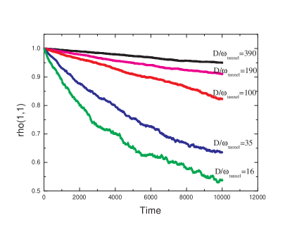
Figure 6: “Watched Pot” effect. Same conditions as in Fig. 5 but with various degrees of strong decoherence ${D}/{\omega_{tunnel}}>>1$. The “freezing” of the evolution is observed as predicted us from Eq 12 with $\rho(1,1)\approx 1-\frac{1}{2}(\omega_{tunnel}^{2}/D)t$. The time interval shown would correspond to about seven undamped oscillations. The different values of $D$ were produced by varying $\Delta$ from 0.01 to 0.002 and calculated from Eq 27.

V.9 Noise Frequency

According to Eq 27, changing $\Delta^{2}$ and $\omega_{c}$ such that their ratio remains constant should leave D the same. However, the higher frequency components of the noise spectrum may have an independent effect through the excitation of higher states. Excitations beyond the lowest states would be undesirable, as it represents a non-unitary evolution among the lowest states, with some probability going to higher states.

On the other hand, if the frequency of the noise is much less than the frequency corresponding to the distance to the next set of levels, the adiabatic theorem tells us that the states remain in the lower set and that such non-unitary effects are suppressed. Since our principal level splittings are generally substantial fractions of unity, there should be little excitation of higher states for noise frequencies $\omega_{c}<<1$. In a plot of the type Fig. 4, excitation of higher states is manifested by the decay of the density matrix element to a value less than 1/2, showing population beyond the first two states.

To examine these points, we show in Table III a series of runs at constant $\Delta^{2}/\omega_{c}$, but different $\omega_{c}$. The resulting D as determined from a fit as in Fig. 4 and the final $\rho(1,1)$ are shown. The approximate constancy of D seems to be well verified. For $\omega_{c}<<1$ the decay is indeed to 1/2, but for larger values there are noticeable departures. In another set of runs with $\Delta$ reduced by a factor of two this effect is almost entirely absent. With our typical time unit these values of D corresponds to a decoherence time of $(1/D)\times 6.3\times 10^{-12}s=3.5ns$ and 14 ns. It should be noted that our noise spectrum has a relatively strong high frequency tail $\sim 1/\omega^{2}$ as opposed to the exponential cutoff one would expect for a purely thermal background.

The actual value of D is of course our great unknown, and we treat it as simply a phenomenological parameter. For orientation we can keep in mind the estimate $D=T/(e^{2}R)$ which we have used previously; or measurements by direct observation of the damped oscillations mooj on a similar SQUID system. These find a decoherence time $\approx 20$ ns at 25mK. This corresponds to the reasonable value $R=260\,k\Omega$ for the effective resistance. Our sample values of $t_{dec}=1/D\sim 10^{3}$ in the dimensionless units, with our typical time unit of $6.3\times 10^{-12}sec$, would correspond to some nanoseconds or tens of nanoseconds for $t_{dec}$.

VI Decoherence in the NOT gate

Having checked that our noise/decoherence simulation has reasonable features, we now turn to some applications. The one variable or one-qubit problem is the simplest situation. When $\phi^{ext}$ is swept (from a relatively large value in the sense $V_{z}>>V_{x}$) to its opposite value, interchanging “up” and “down”, it represents the logic gate NOT. The understanding of the effects of decoherence here is important both for finding the regime of operation of the logic gate and for our proposal deco for measuring D via the success or failure of an adiabatic inversion.

$\omega_{c}$	$\Delta$	D, fit	D, Eq 27	final $\rho(1,1)$
2.0	0.0020	0.0017	0.0018	0.35
0.50	0.0010	0.0017		0.40
0.11	0.00045	0.0018		0.48
0.050	0.00032	0.0018		0.50
0.025	0.00023	0.0019		0.50

Table 3: Values of D and final $\rho(1,1)$ for runs as in Fig. 4, with varying $\omega_{c}$ but constant $\Delta^{2}/\omega_{c}$. The prediction of an approximately constant D, as well as the value for D, are in agreement with Eq 27. The relaxation to a value below 1/2 for the larger $\Delta$ and $\omega_{c}$ values indicates excitation of the third and fourth levels.

In some applications of the adiabatic idea in quantum computing a special role is assigned to the ground state, as in the search for the minimum of a complicated functionalfahri . However our simple gates are not of this type and both states of the qubit, either the ground state or the first excited state, are on an equal footing. Thus in the NOT operation, for example, it is equally important that $1\to 0$ or $0\to 1$, and which of these is represented by the ground state is of no particular significance.

As in the discussion concerning adiabaticity, we measure the “success” of a sweep by the value of “final overlap” as in Fig. 3, where now there is an average over realizations of the random noise. Table IV shows the effects of increasing sweep time with fixed noise parameters. The sweeps are sufficiently long, according to Table II, that non-adiabaticity should be unimportant.

Interestingly, although the noise parameters have been chosen to give a decoherence time of 29 000 time units, Table IV shows decoherence not fully setting in until significantly longer sweep times. This may be understood in terms of our remarks in connection with Eq 13 that decoherence has most of its effect during level crossing. If one attempts to estimate the time spent during the sweep in the vicinity of the “crossing” with the given conditions, it is on the order of 10%. This suggests that the relevant time for the onset of significant decoherence is not 29 000 time units but rather more like 290 000, in agreement with the behavior in Table IV. This argument is supported by examination of Fig. 3 or Fig. 13, where one sees that the actual switching of a state takes place in a small fraction of the total sweep time. Hence for our sorts of logic gates, the speed needed to avoid decoherence may be less stringent than one might simply infer from comparing the sweep time to the decoherence time.

$\beta$	$\xi$	initial $\phi^{ext}$	$\omega_{c}$	$\Delta$	$t_{sweep}$	final overlap
1.19	16.3	0.0020	0.042	0.000042	30 000	0.95
					60 000	0.96
					80 000	0.90
					150 000	0.85
					800 000	0.60
					1 000 000	0.58
					2 000 000	0.52

Table 4: Effect of decoherence on the “success” of adiabatic inversion sweeps. Noise parameters are chosen to give a decoherence time $t_{dec}=1/D=29000$ time units. “Final overlap ” is the average of the overlap squared $\frac{1}{N}\Sigma_{a}|<\psi^{a}|\psi_{f}>|^{2}$ or equivalently $<\psi_{f}|\rho|\psi_{f}>$. As the sweep is made slower, so that decoherence has time to take effect at level crossing, $\rho$ approaches the totally incoherent value of 1/2. Errors on “Final overlap ” are on the order of a few percent. For the no-decoherence situation see Fig. 3 and Table II.

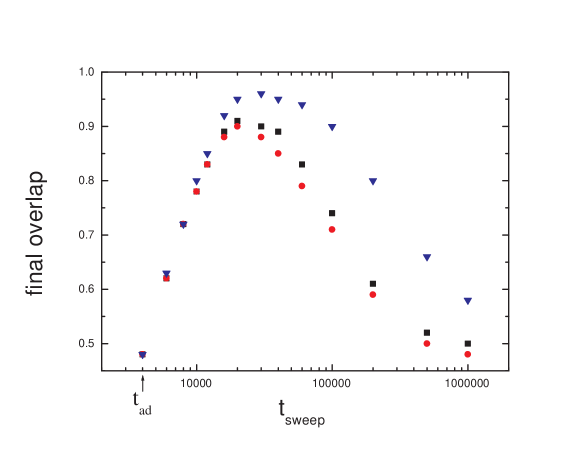
Figure 7: Adiabatic and decoherence effects on the “success” of a sweep ($-0.002\to 0.002$) in $\phi^{ext}$ , for the one dimensional system (NOT) as the sweep time is increased. The adiabatic time for 50% “success” is indicated by an arrow. As the sweep time is lengthened one observes the onset of adiabaticity, followed by decreasing “success” as the decoherence takes effect. Squares and dots: noise parameters adjusted to give $D=1.3\times 10^{-4}$. Squares: $\omega_{c}=20mK$ and $\Delta=5.0\times 10^{-5}$. Dots: $\omega_{c}=50mK;~{}\Delta=7.9\times 10^{-5}$. Triangles: noise parameters adjusted to give $D=3.5\times 10^{-5}$, using $\omega_{c}=50mK$ and $\Delta=4.2\times 10^{-5}$. SQUID parameters are $\beta=1.19,\xi=16.3$.

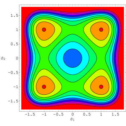
Figure 8: Potential contours for Eq 30, showing the four minima of the 2-qubit system.

To illustrate the effects of non-adiabaticity and decoherence together, we show in Fig. 7 a series of simulations for varying sweep times and $\Delta$’s. There appears to be a broad range around twenty thousand time units where neither effect is drastic. The times refer to our dimensionless units, so for our typical time unit $6.3\times 10^{-12}s$, the two values of D in the plot would correspond to $1/D=t_{dec}=$50 ns and 180 ns. If one were to consider SQUID parameters giving a larger $\omega_{tunnel}$ and so a shorter adiabatic time, the favorable region could be widened considerably to the left, i.e. to shorter times. (See the discussion below “Smaller $\beta$”)

VII Two variable system

We now turn to the two variable or two-qubit system. When two one variable systems are weakly coupled we arrive at a two variable system with four low lying states. For the SQUID these would be the four possible states arising from the current circulating clockwise or counterclockwise in two SQUIDs, and as explained in ref pla this can be so arranged that the result of the sweep of one of the $\phi^{ext}$depends on the state of the other SQUID, thus providing the conditions for a CNOT gate ave . We recall ref1 pla the Hamiltonian for this problem

$$H={-1\over 2\mu_{1}}{\partial^{2}\over\partial\phi^{2}_{1}}+{-1\over 2\mu_{2}}{\partial^{2}\over\partial\phi^{2}_{2}}+V\;,$$ (29)

with $V$

$$V=V_{0}\{{1\over 2}[l_{1}(\phi_{1}-\phi^{ext}_{1})^{2}+l_{2}(\phi_{2}-\phi^{ext}_{2})^{2}-2l_{12}(\phi_{2}-\phi^{ext}_{2})(\phi_{1}-\phi^{ext}_{1})]+\beta_{1}cos\phi_{1}+\beta_{2}cos\phi_{2}\}\;.$$ (30)

In place of $\mu=V_{0}$ for the one variable case, one now has $\sqrt{\mu_{1}\mu_{2}}=V_{0}$. Analogously to the single variable case, the factor $E_{0}$ which converts the energy of the dimensionless Hamiltonian to physical energy involves the inductance and capacitance of the two SQUIDs ref1 , namely $E_{0}=1/\surd LC$, where ${1\over L}={\sqrt{L_{1}L_{2}}\over L_{1}L_{2}-L^{2}_{12}}$ and $C=\sqrt{C_{1}C_{2}}$. The small $l$ are the inductances refered to $L$. In Fig. 8 we reproduce a contour plot for the potential showing its four minima, corresponding to the four states of the 2-qubit system.

As in the one dimensional case, the numerical calculations use a large harmonic oscillator basis, now in two variables. For most runs a basis of one or two thousand states was used. Even when using the “second cut” reduced basis to four eigenstates, time dependent runs with many samples could take several minutes on fast PC’s. It seems that extensions to more than two or three variables would need new computational methods.

A basis for the four states is provided by “spin up(1)spin down(2)=$u_{+}(1)u_{-}(2)$ and so forth:

$$u_{-}(1)u_{-}(2)~{}~{}~{}~{}~{}~{}~{}~{}~{}~{}~{}~{}~{}~{}~{}~{}~{}~{}u_{+}(1)u_{-}(2)~{}~{}~{}~{}~{}~{}~{}~{}~{}~{}~{}~{}~{}~{}~{}~{}u_{-}(1)u_{+}(2)~{}~{}~{}~{}~{}~{}~{}~{}~{}~{}~{}~{}~{}~{}~{}u_{+}(1)u_{+}(2)\;.$$ (31)

These four states correspond to definite senses for the currents in the SQUIDs.

On the other hand if the parameter $l_{12}$ giving the flux coupling between the SQUID is very small, the situation reduces to two independent single variable systems. Thus for the analysis of weak coupling with small $l_{12}$ it is convenient to introduce the eigenstates for any value of the individual $\phi^{ext}$ for each SQUID:

$$v_{-}(1)v_{-}(2)~{}~{}~{}~{}~{}~{}~{}~{}~{}~{}~{}~{}~{}~{}~{}~{}~{}~{}v_{+}(1)v_{-}(2)~{}~{}~{}~{}~{}~{}~{}~{}~{}~{}~{}~{}~{}~{}~{}~{}v_{-}(1)v_{+}(2)~{}~{}~{}~{}~{}~{}~{}~{}~{}~{}~{}~{}~{}~{}~{}v_{+}(1)v_{+}(2)\;.$$ (32)

This is the independent SQUID basis, where each SQUID can have its own Hamiltonian, according to its $\phi^{ext}$.

The $v$ are those discussed in connection with Table I: $v_{+}=(cos\frac{\theta}{2}\,u_{+}+sin\frac{\theta}{2}\,u_{-})$ and $v_{-}=(cos\frac{\theta}{2}\,u_{-}-sin\frac{\theta}{2}\,u_{+})$ . If the applied $\phi^{ext}$are different, then we have different angles $\theta_{1}$ and $\theta_{2}$ in these relations. At $l_{12}=0$ the $v(1)v(2)$’s are the eigenstates of the complete system, and with $l_{12}\neq 0$ there will be a mixing among them.

VIII coupled Hamiltonian in the spin picture

In the spin picture for Eq 30 there are now two “spin 1/2” objects, interacting through $l_{12}$ and subject to the external fields $\phi^{ext}_{1},\phi^{ext}_{2}$. By the arguments used for Eq 4, we make the identifications

$$\phi_{1}\to\phi_{c}(1)\sigma_{z}(1)~{}~{}~{}~{}~{}~{}~{}~{}~{}~{}~{}~{}~{}~{}~{}~{}~{}~{}~{}~{}~{}~{}\phi_{2}\to\phi_{c}(2)\sigma_{z}(2)\;,$$ (33)

and the effective spin Hamiltonian is

$${\textstyle\frac{1}{2}}\,{\bf\sigma}(1)\cdot{\bf V}_{1}+{\textstyle\frac{1}{2}}\,{\bf\sigma}(2)\cdot{\bf V}_{2}-V_{0}l_{12}\biggl{(}\phi_{c}(1)\sigma_{z}(1)-\phi^{ext}_{1}\biggr{)}\biggl{(}\phi_{c}(2)\sigma_{z}(2)-\phi^{ext}_{2}\biggr{)}\;.$$ (34)

Figure 9: Left: Square of the wavefunction for state 1 localized in the lower left potential well of Fig. 8. Right: at “level crossing” as the wavefunction moves to the lower right potential well. Potential parameters were $l_{1}=l_{2}=1,l_{12}=0.005$, $\beta_{1}=\beta_{2}=1.19$ and $V_{0}=16.3$.

For small $l_{12}$ the components of the $\bf V$ are determined as in Eq 6, namely $V_{z}\approx 2V_{0}\,l\,\phi_{c}\phi^{ext}$ while $V_{x}$ is found via Eq 7. As before, $\phi_{c}$ is approximately the $\phi$ of a state localized in one of the potential wells. The effective interaction Hamiltonian between the two devices is then

$$H_{int}\approx-V_{0}l_{12}\phi_{1}\phi_{2}\approx-V_{0}l_{12}\phi_{c}(1)\phi_{c}(2)\sigma_{z}(1)\sigma_{z}(2)\;.$$ (35)

This operator induces level shifts of the four $u$ base states without mixing them. However when the tunneling is introduced as a perturbation, non-trivial combinations of the four states can arise.

VIII.1 Low-lying level patterns

We begin with weakly interacting SQUIDs, $l_{12}<<l_{1},l_{2}$. The energy level pattern anticipated for the lowest levels may be understood by beginning with the totally decoupled system of just two independent devices, $l_{12}=0$. If we take both devices with about the same parameters, for example, we have first the ground state where both SQUIDs are in their lowest state, the first state of Eq 32. Then there are two approximately degenerate states with one SQUID in the first excited state and the other in its ground state, the second and third states of Eq 32. Finally the fourth state has both SQUIDs in the first excited states, the last wavefunction of Eq 32. If each device is in the configuration where the splitting of its first two states is small (small $V_{z}$), as in our discussions above, then the splitting from the ground state to the degenerate pair is equal to the splitting from the pair to the fourth state. Furthermore the splitting to the fifth state should be substantially greater since it involves an excitation of the principal quantum number.

Turning on a small $l_{12}$, we show an example from numerical calculations in Table V. With $l_{12}=10^{-5}$ these reveal the expected pattern. One sees that the fifth state is well separated from the lower ones, again supporting the use of the picture of an approximately isolated Hilbert space, as for the first two states in the single variable case.

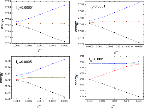
Figure 10: Level behavior for the first four states of two identical SQUIDs with coupling $l_{12}$. In the first panel one notes the pattern of a ground state, an almost degenerate pair and single state, as would be expected for two independent SQUIDs. This pattern changes as the interaction energy between the SQUIDs $\sim V_{0}l_{12}$ becomes on the order of the splitting $\omega_{tunnel}$.

In the example of identical parameters for both SQUIDs, with second and third levels degenerate for $l_{12}=0$, we may use degenerate perturbation theory to find the splitting induced by turning on $l_{12}$. The matrix element is $<v_{+}(1)v_{-}(2)|H_{int}|v_{-}(1)v_{+}(2)>=V_{0}l_{12}(sin\theta)^{2}$, where $\theta$ is the angle for going from the $u$ to the $v$ as discussed in connection with Table I. The splitting of levels 2 and 3 is then $2V_{0}l_{12}(sin\theta)^{2}\phi_{c}^{2}$. With our typical parameters and $l_{12}=1\times 10^{-5}$ and $\phi^{ext}$=0 and so $sin\theta=1$, the formula, using $\phi_{c}\approx 0.88$, gives $25\times 10^{-5}$. The numerical calculation, as shown in Table V, gives $27\times 10^{-5}$.

Observation of this small splitting would be quite amusing with regard to the question of coherence between macroscopic objects. While work with the “Cooper-pair box”pash has seen effects involving interference between the states of two qubits, the states involved differ only microscopically, namely by a Cooper-pair. Here, with the SQUID, the states concerned differ by the circulation direction of a macroscopic number of electrons, and so seem to pose the macroscopic coherence question more dramatically. The energy eigenstates resulting from the diagonalization to obtain the small splitting are $(1/\surd 2)\bigl{(}v_{-}(1)v_{+}(2)\pm v_{+}(1)v_{-}(2)\bigr{)}$. The splitting, one might say, results from the relative quantum phase $\pm$ involving the two SQUIDs, that is, between two macroscopic objects. This is yet a step further than the effects for one SQUID, where one is sensitive to the phase between different macroscopic current directions, but in one device. Since this splitting is very small, however, line broadening due to the noise effects may be comparable to the splitting. Values of $D\sim 10^{-4}-10^{-5}$ for the tens of mK region could be in the same range as the splitting for $l_{12}\sim 10^{-5}$.

The degenerate perturbation theory formula only applies when we have the picture of two approximately degenerate levels well separated from the others, as in Table V. The picture changes rapidly as the mutual coupling $l_{12}$ is increased. In Fig. 10 we show the energy level patterns for the first four levels for different $l_{12}$ as functions of a common applied $\phi^{ext}$. Again, the two SQUIDs are taken to be identical, with our standard parameters. One observes that after about $l_{12}\approx 10^{-4}$ the uncoupled SQUID pattern no longer holds, since now the interaction energy $\sim V_{0}l_{12}$ is on the same order as the original splittings, $\omega_{tunnel}=0.0044$. A characteristic change of behavior occurs when $l_{12}\approx$$\phi^{ext}$. This may be understood as the value of $l_{12}$ where the flux contributed from the other SQUID becomes comparable to the applied $\phi^{ext}$.(see Eq 5 of ref pla ).

Another limit which is not difficult to analyze is that of small $\theta$ or relatively large $\phi^{ext}$(see Table I). In this limit the $u$’s are the eigenstates and the interaction Eq 35 simply gives additive contributions to the energies. We may even consider different parameters and $\phi^{ext}$  for the SQUIDs. According to Eq 34 this results in a ground state with both spins “down” and energy $\frac{1}{2}(-V_{z}(1)-V_{z}(2)-\delta)$ and an upper state with both spins “up” and energy $\frac{1}{2}(+V_{z}(1)+V_{z}(2)-\delta)$. There are two middle states with energy $\frac{1}{2}(+V_{z}(1)-V_{z}(2)+\delta)$ and $\frac{1}{2}(-V_{z}(1)+V_{z}(2)+\delta)$; $\delta$ is the contribution from Eq 35, $\delta=V_{0}l_{12}\phi_{c}(1)\phi_{c}(2)$. In the case of identical SQUIDs these middle states form a degenerate pair, as one sees for the larger $\phi^{ext}$. With small deviations of the $\bf V$ from the z-direction there will again be a splitting which can be found from perturbation theory.

IX CNOT configurations

Our design for a CNOT operation consists of an adiabatic sweep from a point with relatively large $\phi^{ext}$  in the $(\phi^{ext}_{1},\phi^{ext}_{2})$ plane to another such point so that there is a definite mapping among the four $u(1)u(2)$ states. The four possible configurations of currents clockwise and counterclockwise in the two SQUIDs undergo a certain definite, reversible, rearrangement. This rearrangement is chosen in accordance with the definition of CNOT: one pair of states remains unchanged (control bit is zero), while the other pair reverses (control bit is one). This is accomplished by having the energy eigenstates (1,2,3,4), each one concentrated in a different potential well, move from one set of locations to another pla . Since for relatively large $\phi^{ext}$each well represents a distinct state of the SQUID currents, one physical configuration of the two qubits is mapped to another. These rearrangements are represented by “tableaux” like $\pmatrix{3&4\cr 1&2}$ showing the localization of the first four energy eigenstates in the potential wells of Fig. 8.

$\beta$	$\mu$	$l_{12}$	$\phi^{ext}$	$\Delta~{}E$
1.19	16.3	0.00001	0.0	0.0043
				0.00027
				0.0043
				0.42

Table 5: Splittings at $\phi^{ext}$=0 among the first five levels for the first panel of Fig. 10. The energy difference $\Delta E$ is with respect to the previous level, thus the first excited state is 0.0043 units above the ground state. The fifth state is distinctly separated from the first four. The first and third splitting should be approximately that of a single SQUID, which with $\phi^{ext}$=0 is 0.0044. The small splitting between the second and third state is in agreement with the prediction of degenarate perturbation theory, $2V_{0}l_{12}\phi_{c}^{2}$.

In a first step it is only necessary to identify those locations of the $(\phi^{ext}_{1},\phi^{ext}_{2})$ plane with different tableaux such that a sweep from one to the other leads to the desired rearrangement. An example is $\pmatrix{3&4\cr 1&2}\to\pmatrix{4&3\cr 1&2}$. The lower row may be identified with control bit zero, and the upper row with control bit one. The adiabatic theorem then guarantees that a “sufficiently slow” sweep will preserve the occupation of the levels, $1\to 1,2\to 2$ and so forth. Once having so identified the desired sweep, the adiabaticity may be examined afterwards.

Not all points of the $(\phi^{ext}_{1},\phi^{ext}_{2})$ plane are suitable starting or ending points for a sweep since we require “well defined” wavefunctions. The wavefunctions should be A) well localized in one potential well so that the SQUID is in a definite flux state, and B) all first four states should be localized in different wells. Fig. 9 shows the appearance of a “good wavefunction ” with state 1 in the lower left potential well of Fig. 8. In the searches a wavefunction was considered as “well localized” when the distance between centers of the wavefunctions was more than 2.5 times the spread of the wavefunction, as measured by the dispersion.

In Fig. 11 we show the results of such a search. The associated tableaux are indicated for each region. The black areas are those of “bad wavefunctions ”. The general range of “good” corresponds to the observations for one SQUID in Table I, where the spin picture was valid up to about $\phi^{ext}$$\approx 0.01.$

In principle a CNOT may be accomplished by a sweep between any two adjacent regions where one row (or column) interchanges and the other does not. As was explained in ref.pla , the switching values between tableaux (dark lines) may be understood as a “level crossing” occurring when the flux from the control SQUID onto the target SQUID is equal and opposite to the applied flux onto the target SQUID. That is, when $\phi^{ext}$$=l_{12}/l$. At this point the total flux on the target SQUID is approximately zero and so is at a level crossing. This argument allows one to understand the pattern of dark lines. It will be noted that in crossing a dark line only adjacent energy levels switch, as expected for a “crossing”. The vertices are singular points involving more than two levels.

For a smaller $l_{12}$ the map will then be similar but with smaller regions between the vertical and horizontal dark lines. In the central box of the plot, although there are “good” wavefunctions, the applied flux is apparently too low for the “immobilization” argument of ref. pla to work and there are no CNOT rearrangements within the box. However CNOT sweeps exist connected to peripheral regions. These take place in the vertical or horizontal direction with the flux on one qubit (control bit) relatively large and constant while the other flux (target bit) is varied.

For such vertical or horizontal sweeps, involving changing one flux, only one SQUID inverts, according to which one undergoes the sweep. In diagonal sweeps involving both fluxes on the other hand, states transfer across the diagonal in the tableaux, indicating changes in both SQUIDs. This explains why the diagonal black lines are very narrow, since such “double flips” involve two tunnelings with a corresponding small mixing energy.

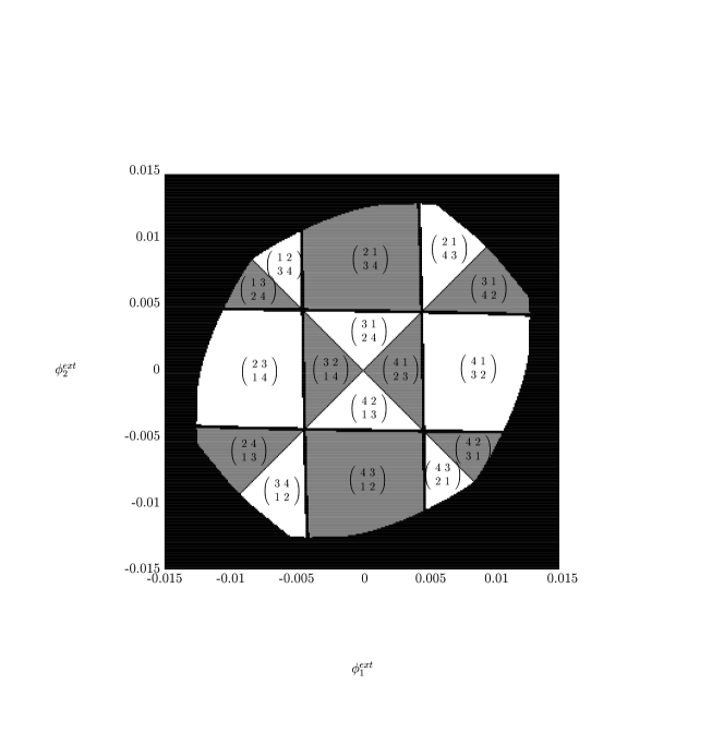
Figure 11: Map of the regions of $(\phi^{ext}_{1},\phi^{ext}_{2})$plane with well defined wavefunctions suitable for performing CNOT. The numbers in a tableaux show the location of the first four energy eigenstates on the potential landscape of Fig. 8. These show that a CNOT may be obtained by horizontal or vertical sweeps in the regions external to the central square. Potential parameters used were $l_{1}=l_{2}=1,l_{12}=0.005$, $\beta_{1}=\beta_{2}=1.19$ and $V_{0}=16.3$.

Figure 12: Region of the $(\phi^{ext}_{1},\phi^{ext}_{2})$ plane with high “completeness ” using Eq 36. One notes the close similarity to the region defined by Fig. 11, which was found by examination of individual wavefunctions.

Although the map of Fig. 11 was obtained by an examination of the individual wavefunctions, a reasonable idea may be had by simply inspecting the potential landscape. Since the ordering of the energy levels will usually follow the ordering of the minima of the potential wells, we find that the ordering of the minima usually give the correct tableaux. Thus a suitable sweep is frequently simply one where the potential minima rearrange in the desired manner. Alternatively, all the transition lines on the map may be found from the set of linear relations arising from the “level crossing” conditions (coefficients of the $\sigma_{z}$) while treating the tunneling ($\sigma_{x}$) terms as a perturbation.

IX.1 Hilbert space completeness

For the “spin 1/2 picture” to be a meaningful in a complex system with many levels it is necessary that the states selected constitute an approximately independent vector space. If, for example, the selected states were to mix with other states of the system as we carry out our gate operations, then the two states would not be a faithful representation of a two-state qubit, since more than two states would be involved. And similarly when we have two qubits or four states for CNOT, these four should act effectively as a separate space.

The Hilbert space completeness test mentioned at the end of the section “Identification with a spin 1/2 system” proves to be quite interesting in this regard and may be a useful tool in studying higher dimensional systems. In this method, we take a point in the parameter space of the Hamiltonian and compare it with some reference point. If the Hilbert spaces for these different Hamiltonians are closely the same, there should be a high overlap of the lowest eigenstates for the different Hamiltonians. As we shall explain, a test can formulated which applies to any linear combination. For the one variable system the parameter space in question is the $\phi^{ext}$ line, and with two variables the $(\phi^{ext}_{1},\phi^{ext}_{2})$ plane. The precise point we choose as the reference is unimportant in regions where the overlaps are high; for the $(\phi^{ext}_{1},\phi^{ext}_{2})$ plane we take $(\phi^{ext}_{1},\phi^{ext}_{2})$=(0,0).

Let the $v_{i}$ be the lowest eigenstates at the reference point and $v^{\prime}$ a linear combination of the lowest eigenstates for some other parameter values. We search for the “worst case”, the minimum value of $\Sigma|<v_{i}|v^{\prime}>|^{2}$. The procedure involves constructing the matrix $M_{ij}=<v_{i}|v^{\prime}_{j}>$. For the one SQUID or two state system i and j run from one to two; in the two variable system from one to four.

One now observes that the sum of the overlaps squared $\Sigma|<v_{i}|v^{\prime}>|^{2}$ is the expectation of the matrix $M^{T}M$ in the state $|v^{\prime}>$. Thus the worst or lowest overlap for an arbitrary normalized linear combination in the $v^{\prime}$ space is given by the lowest eigenvalue of this matrix:

$$least~{}overlap=smallest~{}eigenvalue~{}M^{T}M$$ (36)

Varying the chosen point in the $(\phi^{ext}_{1},\phi^{ext}_{2})$  plane, one maps out the region of a common Hilbert space where the worst overlap is close to one. Fig. 12 shows such a map, produced with high resolution. A grey scale was used for the points, from white for $least~{}overlap=1$ to black for $least~{}overlap=0$.

It is quite interesting that the region of the $(\phi^{ext}_{1},\phi^{ext}_{2})$plane found by this method is essentially the same as that found by the detailed examination of individual wavefunctions as in Fig. 11. This may perhaps be understood by noting that if we have “bad wavefunctions ” with two states in one potential well, this will have a poor overlap with the “good” situation where each wavefunction is in a different well. On the other hand “bad wavefunctions ”in the sense that they are delocalized, as at a “crossing”, will still give a high “completeness”. The sharp transition, with little grey area, seems remarkable. Although the corresponding transition in the one dimensional case was rather abrupt, it seems more so here, presumably the effect is multiplicative. Both Figs. 11 and 12 contain 90 000 pixels, necessitating runs of many hours.

Fig. 12 does not contain the narrow black bands of Fig. 11, where there are “bad wavefunctions ” at “level crossings”. This is because these “bad wavefunctions ”, although delocalized in $\phi$ and so not corresponding to a definite state of the SQUIDs, are still in the same Hilbert space as the localized states. An example of such a state is shown in the Right panel of Fig. 9. It should also be noted that the narrowness of the black bands in Fig. 11 is in accord with our earlier remarks concerning the small fraction of the time spent near “crossing” during a sweep.

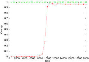
Figure 13: Behavior of the states 1 and 4 in a CNOT sweep connecting two tableaux, where state 1 should remain in its original location while state 4 should reverse, as in the lower left of Fig. 11. No noise is applied. The vertical axis shows the overlap of the wavefunction with its intended final state. State 1 (upper curve) should not change its location and is seen to be stable. State 4 (lower curve) should reverse its location and is seen to go from zero to approximately complete overlap with the desired final state. State 2 and state 3 are not shown but behave similarly to states 1 and 4 respectively. Squid parameters are as in Fig. 11, and the sweep time was 20 000 units. It is to be observed that the switch itself takes place in a small fraction of the sweep time.

IX.2 Noise for the two variable system

The extension of the previous noise treatment to the two variable problem is straightforward if we continue to represent the noise as fluctuations of the external fluxes $\phi^{ext}$. To each $\phi^{ext}$  there will now be a noise term as in Eq 15. As in the discussion of Eq 34 we have $V_{z}\approx 2V_{0}l\phi^{ext}\phi_{c}$ and so an additional term in Eq 34

$$-V_{0}\{l_{1}\phi_{c}(1)\sigma_{z}(1){\cal N}_{1}+l_{2}\phi_{c}(2)\sigma_{z}(2){\cal N}_{2}\}\;,$$ (37)

where again we keep only the linear term in the noise.

There will then be a $D$ as in Eq 27 associated with each variable

$$D_{1}=4{(V_{0}l_{1}\phi_{c}(1)\Delta_{1})^{2}\over\omega_{c}(1)}~{}~{}~{}~{}~{}~{}~{}~{}~{}~{}~{}~{}~{}~{}~{}~{}~{}D_{2}=4{(V_{0}l_{2}\phi_{c}(2)\Delta_{2})^{2}\over\omega_{c}(2)}\;.$$ (38)

We can now carry out the simulations with the two noise signals imposed, one for each SQUID.

X CNOT sweeps

As for the one-bit case, the “success” of a sweep can be measured by the overlap of an evolved wavefunction with the stationary eigenstate for the intended final state. For CNOT two wavefunctions, representing control bit =0, should not change their states, while those representing control bit =1 should move to new positions. We exemplify a successful CNOT sweep in Fig. 13 where we show the behavior of states 1 and 4 for a sweep between a tableaux $\pmatrix{3&4\cr 1&2}$ and a tableaux $\pmatrix{4&3\cr 1&2}$. One sees the reversal of state 4 while state 1 remains steady.

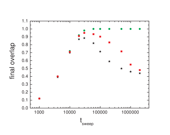
Figure 14: A CNOT sweep in the lower right of the $(\phi^{ext}_{1},\phi^{ext}_{2})$  plane of Fig. 11, with $(0,-0.01)\to(0.006,-0.01)$. The final overlap is plotted for state 1, which should change position. The coupling between the SQUIDs is $l_{12}=0.005$. The sweep without noise (circles) shows the effect of non-adiabaticity for fast sweeps, while the addition of noise exhibit the noise/decoherence effects at longer times. The squares have noise parameters $\Delta=0.000042,\,\omega_{c}=0.042$ and the stars $\Delta=0.000079,\,\omega_{c}=0.042$. The noise is applied to both SQUIDs equally but independently.

In Fig. 14 we illustrate the effects of non-adiabaticity and decoherence for the $\pmatrix{4&3\cr 1&2}\to\pmatrix{4&3\cr 2&1}$ sweep of the right lower portion of Fig. 11, with $(0,-0.01)\to(0.006,-0.01)$. The curves show the behavior of the overlap for state 1, which ideally would behave as the switching curve of Fig. 13, reaching close to complete overlap. The upper curve, without noise, shows the progression to adiabaticity as the sweeps become slower. The lower curves have noise applied, equally to both SQUIDs, to show the effects of decoherence. The two sets of noise parameters, according to Eq 38, correspond to decoherence times of 29 000 and 8 200 time units, giving decoherence times 1/D of 180ns and 52ns with our typical time unit. In terms of the formula $1/D=e^{2}R/T$, at 20mK these would correspond to $R\approx 2M\Omega$ and $R\approx 580k\Omega$. As expected, the wavefunctions for the states which should not change remained stable in these runs.

In these runs we applied the noise to each SQUID independently. However, one might consider the effects of a common noise applied to both SQUIDs together. This would be the case not for the true intrinsic decoherence but could represent, say, an instrumental effect due to an external common noise like long range fluctuations in the applied field. Interestingly, applying the noise signal so it is the same on both devices seems to have little or no effect. Taking the lower curve of Fig. 14 at $t_{sweep}=100\;000,$ one finds that such a common noise produces the same result as the independent noise, namely a final overlap of 0.7. This at first surprising result is understandable from the fact that the major effect of the noise takes place at level crossing. The noise is mostly effective on the SQUID undergoing the sweep and apparently the noise on the control SQUID has little effect. Indeed, turning the noise on SQUID 2 completely off still leaves the final overlap at 0.7; but turning it off for SQUID 1 leads to a perfect result with overlap $\approx$ 1.

XI Smaller $\beta$

As seen in Table II, a reduced $\beta$ gives an increased $\omega_{tunnel}$ and shorter adiabatic times. Since shorter times gives the decoherence less time to act, there is reduced decoherence. This suggest examining the situation with a reduced tunnel barrier. We take $\beta=1.14$, which according to Table II, increases $\omega_{tunnel}$ by a factor six, from 0.0044 to 0.027 energy units. Fig. 15 shows, analogously to Fig. 11, the good domains of the $(\phi^{ext}_{1},\phi^{ext}_{2})$plane for $\beta=1.14$. The small change in $\beta$ has great effects. The thin black lines of Fig. 11, with “bad wavefunctions ”, have now become broad bands. Thus starting and finishing points of the sweeps are now restricted to certain “islands”. By lowering the tunnel barrier, we have created substantial areas represented by the Right panel of Fig. 9, where the wavefunctions are not in a single well with a definite flux in the SQUIDs. While for Fig. 11, this occurred only at the “level crossings” given by the black lines, there are now rather large regions with delocalized wavefunctions. Even on the “good” islands examination of pictures of the wavefunctions as in Fig. 9 shows that, while they are generally still well concentrated, there are little ripples some distance off from the center of localization. Evidently in this parameter range we operate on the border to total delocalization.

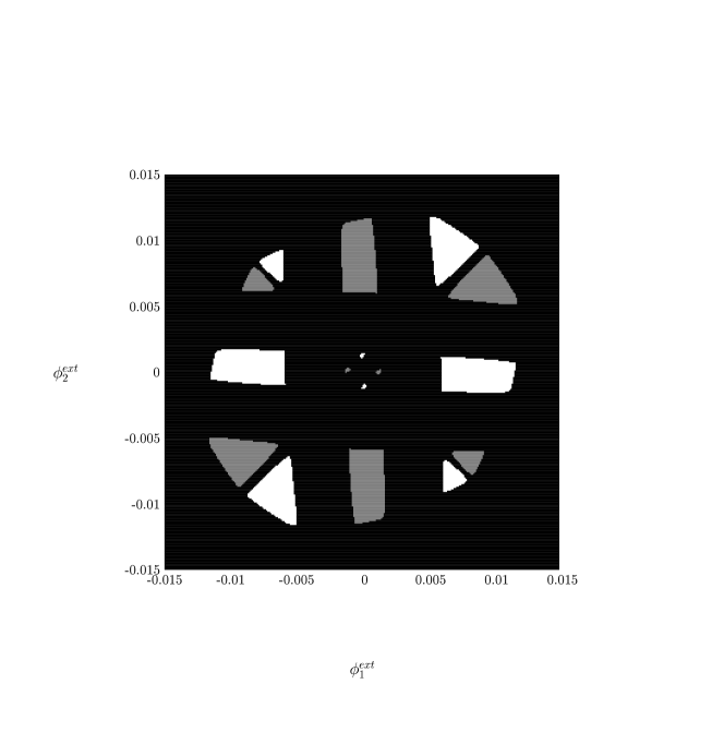
Figure 15: “Good domains” of the $(\phi^{ext}_{1},\phi^{ext}_{2})$  plane as in Fig. 11 with the smaller $\beta$ values $\beta_{1}=\beta_{2}=1.14$. Due to the increased tunneling the “good” regions where there is a definite state of the SQUIDs have been reduced to small islands. The relative narrowness for the diagonal bands, as discussed for Fig. 11, is seen here clearly. For legibility the tableaux are not shown; however they correspond to those on Fig. 11.

To examine the hoped-for improved robustnessrobust with respect to noise/decoherence we show in Table VI the results of a series of CNOT sweeps for $\beta=1.14$, choosing a sweep on the lower left of Fig. 15 where $\pmatrix{3&4\cr 1&2}\to\pmatrix{4&3\cr 1&2}$. The increased $\omega_{tunnel}$ allows us to set $t_{sweep}$ as short as 1 000 units without violating adiabaticity. Increasing the noise parameter $\Delta$ from zero and tabulating the final overlap for state 4, one sees that significantly shorter decoherence times as compared to $\beta=1.19$ (Fig. 14) become possible. The next-to-last entry would correspond to a decoherence time of only 500 time units. This reflects in part the phenomenon discussed in connection with Eq 13 and Table IV that the sweep time can be longer than the decoherence time before large decoherence effects occur.

The 500 time units would be 3.1 ns with our “typical” parameters. This is substantially less than the 20 ns reported in ref. mooj . This is one of our most interesting results concerning the engineering of such devices and perhaps implies that the feasibility of such devices is not so very far off.

$\beta$	$~{}~{}~{}~{}~{}~{}\mu,~{}~{}~{}~{}V_{0}$	$l_{12}$	initial $(\phi^{ext}_{1},\phi^{ext}_{2})$	final $(\phi^{ext}_{1},\phi^{ext}_{2})$	$t_{sweep}$	state	$\Delta$	final overlap
1.14	16.3	0.005	(-0.0080,  -0.0075)	(0.0,   -0.0075)	1 000	4	0.0	0.98
							0.000079	0.98
							0.00016	0.97
							0.00032	0.87
							0.00064	0.68

Table 6: CNOT sweeps with a shortened adiabatic time, using $\beta=1.14$. “Final overlap” is shown for increasing noise parameter $\Delta$. Due to the increased $\omega_{tunnel}$ permitting faster sweeps, a much stronger decoherence, compared to $\beta=1.19$, can be tolerated before the sweeps become unsuccessful. Other parameters are as in Fig. 14. The noise frequency was $\omega_{c}=0.042$. The entry with $\Delta=0.00032$ would correspond to a decoherence time of 500 time units, or 3.1 ns with our “typical” parameters.

XII Conclusions

We have presented a description of one or two interacting rf SQUIDs in a form suitable for numerical simulation and a system of programs for carrying out these simulations. In addition to static properties, the behavior under time dependent conditions, including flux sweeps for adiabatic gates, and the effects of noise or decoherence, were studied.

Among the points investigated was the validity of the “spin 1/2 picture” where the behavior governed by the full Hamiltonian is approximated by the components of an effective “spin 1/2”system using the lowest levels of the double-potential well. The identification between the parameters of the spin Hamiltonian and the full Hamiltonian was established and the regime of validity of the approximation were investigated numerically. It is found, using various criteria, including “Hilbert space completeness”, that the “spin 1/2” picture is approximately valid up to variations of the external bias which moves the basic pair of levels a substantial fraction of the principal level splitting.

For the two SQUID system, we have found it is capable of performing the logical operation CNOT, and have been able to determine regions of the $(\phi^{ext}_{1},\phi^{ext}_{2})$plane with definite configurations of the wavefunctions suitable for CNOT sweeps. The conditions for adiabatic behavior under such sweeps were examined and adiabatic times found for typical SQUID parameters. The splitting $\omega_{tunnel}$ of the basic pair enters into the adiabatic condition and is very sensitive to the barrier parameter $\beta$. It is found that the most interesting regions for this parameter are values slightly greater than one, and detailed studies were presented for $\beta=1.19$.

Noise or decoherence were simulated as a random flux noise and a formula was derived relating the parameters of this random noise to the decoherence parameter D. Numerical simulations verify the validity of the formula. This random noise is then applied to the adiabatic logic gates and possible regimes of operation for the gates are found. One of the interesting conclusions is that the adiabatic sweep time can be substantially longer than the decoherence time 1/D before decoherence effects become very large. This is traced to the fact that decoherence, and also non-adiabaticity, are mostly effective at “level crossing”, which is only a small part of the sweep. Indeed for the two-SQUID CNOT gate it is found that noise applied to the control bit SQUID, which does not undergo a “level crossing”, has almost no effect.

One of our general conclusions therefore, for any devices of this general type, is that “level crossings” should be held to a minimum, and when they occur a large tunneling energy or splitting at “crossing” is beneficial both for reducing both decoherence and non-adiabaticity effects.

It thus appears that an interesting region for the engineering of adiabatic gates involves rather small values of $\beta$, where the splitting is large. However the wavefunctions are then nearly delocalized. We have examined the case $\beta=1.14$, where the reduced tunnel barrier and thus large $\omega_{tunnel}$ permit fast operation of the gates. The resulting short time for the decoherence to act leads to operations which are successful with presently discussed values of the decoherence time, some nanoseconds. However, a careful choice of parameters is necessary.

Generally speaking, we may say that our studies verify that it is in principal possible to have a regime where one can create and manipulate quantum linear combinations of quasi-classical objects, as pictured in Fig. 9.

While the parameters and examples we have used are specific to the rf SQUID, it will be recognized that our methods and results will apply, after some adjustments, to almost all interacting double-potential well systems.

References

- (1) P. Silvestrini and L. Stodolsky, Physics Letters A280 17-22 (2001). See also P. Silvestrini and L. Stodolsky in Macroscopic Quantum Coherence and Quantum Computing, pg. 271, Eds. D. Averin, B. Ruggiero and P. Silvestrini, Kluwer Academic/Plenum, New York; cond-mat/0004472.
- (2) V. Corato, P. Silvestrini, L. Stodolsky, and J. Wosiek, Phys. Rev. B68 224508 (2003); cond-mat/0310386.
- (3) V. Corato, P. Silvestrini, L. Stodolsky and J. Wosiek, Phys. Lett. A309 206 (2003);cond-mat/0205514.
- (4) A review with many of the basic concepts and formulas relevant to the subject, as well as references, is Y. Makhlin, G. Schön and A. Shnirman in Rev. Mod. Phys. 73 2001.
- (5) We express frequencies as angular frequency, radians/second, since this what naturally arises with units. To get Herz, divide by . We take this opportunity to correct a misunderstanding in refs pla ; ref1 ; deco where frequencies were expressed as Hz: the units should have been radians/second. Other quantities, not cited as Hz, need not be changed.
- (6) See Figure 2C of I. Chiorescu , Y. Nakamura, C.J.P. Harmans and J.E. Mooij, Science 299 1868 (2003).
- (7) See the section on “Predissociation” in L. D. Landau and E. M. Lifshitz, Quantum Mechanics, Pergamon Press, 1958.
- (8) R.A. Harris and L. Stodolsky, Phys. Lett. B116 464 (1982). For a general introduction and review of these concepts see L. Stodolsky, “Quantum Damping and Its Paradoxes” in Quantum Coherence, J. S. Anandan ed. World Scientific, Singapore (1990) or L. Stodolsky. “Coherence and the Clock” in Time and Matter, I. I. Bigi and M. Faessler, Eds. World Scientific, (2006), pg. 117; quant-ph/0303024.
- (9) L. D. Landau and E. M. Lifshitz, Quantum Mechanics, Pergamon Press, 1958. For a discussion of the density matrix in the present context see Time and Matter, ref us .
- (10) See, for example. chapter 3 of Threshold Signals, by J. L. Lawson and G.E. Uhlenbeck, Dover, 1950.
- (11) I. Chiorescu , Y. Nakamura, C.J.P. Harmans and J.E. Mooij, Science 299 1868 (2003).
- (12) The method is described in J. Wosiek, Nucl. Phys. B644 85 (2002); hep-th/0203116.
- (13) E. Farhi, J. Goldstone, S. Gutmann, and M. Sipser, quant-ph/0001106.
- (14) Yu. A. Pashkin, T. Yamamoto, O. Astafiev, Y. Nakamura, D. V. Averin and J. S. Tsai, Nature 421 823 (2003).
- (15) D.V. Averin, Solid State Communications 105 659 (1998), suggested using adiabatic “level crossings” to implement the CNOT operation in Josephson devices.
- (16) Increased robustness with respect to decoherence with increased tunnel splitting might, at first sight, appear to be unclear in view of the approach reviewed in section IV B of ref rev , where there seem to be two rates involved with the decoherence, with one of them apparently proportional to the tunnel splitting. However, for small , using one verifies that the two rates Eqs 4.11 and 4.12 of ref rev are really the same, controlled by the same factor . That is, both terms are induced by the same physical processes and there is really only one decoherence parameter. This is in fact represented by our , and at small x our simulations automatically include “both kinds” of decoherence. The assumption of small x ( See discussion following Eq 23) is approximately correct in view of the small tunneling splittings, but for very low temperature where “spontaneous emission” becomes important, the point might have to be reconsidered. This might be handled by modifying our Eq 12 so that with constant the density matrix relaxes not to at infinite time but to the more strictly correct limit given by a Boltzmann factor. Of course, the argument that an increased tunnel splitting allows a faster adiabatic sweep and so less time for decoherence to act remains true, independently of this issue.