Stability and stabilisation of the
lattice Boltzmann method
Magic steps and salvation operations

Abstract

We revisit the classical stability versus accuracy dilemma for the lattice Boltzmann methods (LBM). Our goal is a stable method of second-order accuracy for fluid dynamics based on the lattice Bhatnager–Gross–Krook method (LBGK).

The LBGK scheme can be recognised as a discrete dynamical system generated by free-flight and entropic involution. In this framework the stability and accuracy analysis are more natural. We find the necessary and sufficient conditions for second-order accurate fluid dynamics modelling. In particular, it is proven that in order to guarantee second-order accuracy the distribution should belong to a distinguished surface – the invariant film (up to second-order in the time step). This surface is the trajectory of the (quasi)equilibrium distribution surface under free-flight.

The main instability mechanisms are identified. The simplest recipes for stabilisation add no artificial dissipation (up to second-order) and provide second-order accuracy of the method. Two other prescriptions add some artificial dissipation locally and prevent the system from loss of positivity and local blow-up. Demonstration of the proposed stable LBGK schemes are provided by the numerical simulation of a $1$D shock tube and the unsteady $2$D-flow around a square-cylinder up to Reynolds number $\mathcal{O}(10000)$.

I Introduction

A lattice Boltzmann method (LBM) is a discrete velocity method in which a fluid is described by associating, with each velocity $\mbox{\boldmath$v$}_{i}$, a single-particle distribution function $f_{i}=f_{i}(\mbox{\boldmath$x$},t)$ which is evolved by advection and interaction on a fixed computational lattice.

The method has been proposed as a discretization of Boltzmann’s kinetic equation (for an introduction and historic review see succi01 ). Furthermore, the collision operator can be alluringly simplified, as is the case with the Bhatnager–Gross–Krook (BGK) operator bgk54 , whereby collisions are described by a single-time relaxation to local equilibria $f_{i}^{*}$:

$$\frac{\partial f_{i}}{\partial t}+\mbox{\boldmath$v$}_{i}\cdot\nabla f_{i}=\frac{1}{\tau}(f_{i}^{*}-f_{i}).$$ (1)

The physically reasonable choice for $f_{i}^{*}$ is as entropy maximizers, although other choices of equilibria are often preferred succi01 . The local equilibria $f_{i}^{*}$ depend nonlinearly on the hydrodynamic moments (density, momentum, etc.). These moments are linear functions of $f_{i}$, hence (1) is a nonlinear equation. For small $\tau$, the Chapman–Enskog approximation Chapman reduces (1) to the compressible Navier–Stokes equation succi01 with kinematic viscosity $\nu\sim\tau c_{1}^{2}$, where $c_{1}$ is the thermal velocity for one degree of freedom.

The overrelaxation discretization of (1) (see, e.g., Benzi ; LB1 ; Higuera ; succi01 ; karlin06 ; karlin07 ) is known as LBGK, and allows one to choose a time step $\delta_{t}\gg\tau$. This decouples viscosity from the time step, thereby suggesting that LBGK is capable of operating at arbitrarily high-Reynolds number by making the relaxation time sufficiently small. However, in this low-viscosity regime, LBGK suffers from numerical instabilities which readily manifest themselves as local blow-ups and spurious oscillations.

Another problem is the degree of accuracy. An approximation to the continuous-in-time kinetics is not equivalent to an approximation of the macroscopic transport equation. The fluid dynamics appears as a singular limit of the Boltzmann or BGK equation for small $\tau$. An approximation to the corresponding slow manifold in the distribution space is constructed by the Chapman–Enskog expansion. This is an asymptotic expansion, and higher (Burnett) terms could have singularities. An alternative approach to asymptotic expansion (with “diffusive scaling” instead of “convective scaling” in the Chapman–Enskog expansion) was developed in Junk in order to obtain the incompressible Navier–Stokes equations directly from kinetics.

It appears that the relaxation time of the overrelaxation scheme to the slow hydrodynamic manifold may be quite large for small viscosity: $t_{\rm relax}\sim c_{1}^{2}\delta_{t}^{2}/(2\nu)\sim\delta_{t}^{2}/(2\tau)$ (see below, in Sec. III). Some estimates of long relaxation time for LBGK at large Reynolds number are found earlier in Xiong . So, instead of fast relaxation to a slow manifold in continuous-in-time kinetics, we could meet a slow relaxation to a fluid dynamics manifold in the chain of discrete LBM steps.

Our approach is based on two ideas: the Ehrenfests’ coarse-graining ehrenfest11 ; GKOeTPRE2001 ; gorban06 and the method of differential approximation of difference equations Hirt ; Shokin . The background knowledge necessary to discuss the LBM in this manner is presented in Sect. II. In this section, we answer the question: how to provide second-order accuracy of the LBM methods for fluid dynamics modelling? We prove the necessary and sufficient conditions for this accuracy. It requires a special connection between the distribution $f_{i}$ and the hydrodynamic variables. There is only one degree of freedom for the choice of $f_{i}$, if the hydrodynamic fields are given. Moreover, the LBM with overrelaxation can provide approximation of the macroscopic equation even when it does not approximate the continuous-in-time microscopic kinetics.

This approach suggests several sources of numerical instabilities in the LBM and allows several recipes for stabilisation. A geometric background for this analysis provides a manifold that is a trajectory $\mathfrak{q}$ of the quasiequilibrium manifold due to free-flight. We call this manifold the invariant film (of nonequilibrium states). It was introduced in ocherki and studied further in gorban06 ; Plenka ; GorKar . Common to each stabilisation recipe is the desire to stay uniformly close to the aforementioned manifold (Sect. III).

In Sect. IV, in addition to two LBM accuracy tests, a numerical simulation of a $1$D shock tube and the unsteady $2$D-flow around a square-cylinder using the present stabilised LBM are presented. For the later problem, the simulation quantitatively validates the experimentally obtained Strouhal–Reynolds relationship up to $\mathrm{Re}=\mathcal{O}(10000)$. This extends previous LBM studies of this problem where the relationship had only been successfully validated up to $\mathrm{Re}=\mathcal{O}(1000)$ ansumali04 ; baskar04 .

Sect. V contains some concluding remarks as well as practical recommendations for LBM realisations.

We use operator notation that allows us to present general results in compact form. The only definition we have to recall here is the (Gâteaux) differential: the differential of a map $J(f)$ at a point $f_{0}$ is a linear operator $(D_{f}J)_{f_{0}}$ defined by a rule: $(D_{f}J)_{f_{0}}g=\frac{{\mathrm{d}}}{{\mathrm{d}}\varepsilon}(J(f_{0}+\varepsilon g))_{\varepsilon=0}$.

II Background

Microscopic and macroscopic variables.

Let us describe the main elements of the LBM construction. The first element is a microscopic description, a single-particle distribution function $f(\mbox{\boldmath$x$},\mbox{\boldmath$v$})$, where $x$ is the space vector, and $v$ is velocity. If velocity space is approximated by a finite set $\{\mbox{\boldmath$v$}_{i}\}$, then the distribution is approximated by a measure with finite support, $f(\mbox{\boldmath$x$},\mbox{\boldmath$v$})\approx\sum_{i}f_{i}\delta(\mbox{\boldmath$v$}-\mbox{\boldmath$v$}_{i})$. In that case, the microscopic description is the finite-dimensional vector-function $f_{i}(\mbox{\boldmath$x$})$.

The second main element is the macroscopic description. This is a set of macroscopic vector fields that are usually some moments of the distribution function. The main example gives the hydrodynamic fields (density–momentum–energy density): $\{n,n\mbox{\boldmath$u$},\mathcal{E}\}(\mbox{\boldmath$x$})=\int\{1,\mbox{\boldmath$v$},v^{2}/2\}f(\mbox{\boldmath$x$},\mbox{\boldmath$v$})\,{\mathrm{d}}\mbox{\boldmath$v$}$. But this is not an obligatory choice. If we would like to solve by LBM methods the Grad equations Grad ; HudongGrad or some extended thermodynamic equations EIT , we should extend the list of moments (but, at the same time, we should be ready to introduce more discrete velocities for a proper description of these extended moment systems).

In general, we use the notation $f$ for the microscopic state, and $M$ for the macroscopic state. The vector $M$ is a linear function of $f$: $M=m(f)$.

Equilibrium.

For any allowable value of $M$ an “equilibrium” distribution should be given: a microscopic state $f^{*}_{M}$. It should satisfy the obvious, but important identity of self-consistency:

$$m(f^{*}_{M})=M,$$ (2)

or in differential form

$$m(D_{M}f^{*}_{M})\equiv 1,\quad\text{i.e., $m((D_{M}f^{*}_{M})a)\equiv a$}.$$ (3)

The state $f^{*}_{M}$ is not a proper thermodynamic equilibrium, but a conditional one under the constraint $m(f)=M$. Therefore we call it a quasiequilibrium (other names, such as local equilibrium, conditional equilibrium, generalised canonical state or pseudoequilibrium are also in use).

For the quasiequilibrium $f^{*}_{M}$, an equilibration operation is the projection $\Pi^{*}$ of the distribution $f$ into the corresponding quasiequilibrium state: $\Pi^{*}(f)=f^{*}_{m(f)}$.

In the fully physical situation with continuous velocity space, the quasiequilibrium $f^{*}_{M}$ is defined as a conditional entropy maximizer by a solution of the optimisation problem:

$$S(f)\to\max,\ m(f)=M,$$ (4)

where $S(f)$ is an entropy functional.

The choice of entropy is ambiguous; generally, we can start from a concave functional of the form

$$S(f)=\int s(f(\mbox{\boldmath$x$},\mbox{\boldmath$v$},t))f(\mbox{\boldmath$x$},\mbox{\boldmath$v$},t)\,{\mathrm{d}}\mbox{\boldmath$x$}{\mathrm{d}}\mbox{\boldmath$v$}$$ (5)

with a concave function of one variable $s(f)$. The choice by default is $s(f)=-\ln f$, which gives the classical Boltzmann–Gibbs–Shannon (BGS) entropy.

For discrete velocity space, there exist some extra moment conditions on the equilibrium construction: in addition to (2) some higher moments of a discrete equilibrium should be the same as for the continuous one. This is necessary to provide the proper macroscopic equations for $M$. Existence of entropy for the entropic equilibrium definition (4) whilst fulfilling higher moment conditions could be in contradiction, and a special choice of velocity set may be necessary (for a very recent example of such research for multispeed lattices see Shyam2006 ). Another choice is to refuse to deal with the entropic definition of equilibrium (4) and assume that there will be no perpetuum mobile of the second kind. This extends the possibility for approximation, but creates some risk of nonphysical behavior of the model. For a detailed discussion of the $H$-theorem for LBM we refer the readers to LB3 .

Some of the following results depend on the entropic definition of equilibrium, but some do not. We always point out if results are “entropy–free”.

Free flight.

In the LBM construction the other main elements are: the free-flight transformation and the collision. There are many models of collisions, but the free-flight equation is always the same

$$\frac{\partial f}{\partial t}+\mbox{\boldmath$v$}\cdot\nabla_{x}f=0,$$ (6)

with exact solution $f(\mbox{\boldmath$x$},\mbox{\boldmath$v$},t)=f(\mbox{\boldmath$x$}-\mbox{\boldmath$v$}t,\mbox{\boldmath$v$},0)$, or for discrete velocities,

$$\frac{\partial f_{i}}{\partial t}+\mbox{\boldmath$v$}_{i}\cdot\nabla_{x}f_{i}=0,$$ (7)

$f_{i}(\mbox{\boldmath$x$},t)=f_{i}(\mbox{\boldmath$x$}-\mbox{\boldmath$v$}_{i}t,0)$. Free-flight conserves any entropy of the form (5). In general, we can start from any dynamics. For application of the entropic formalism, this dynamics should conserve entropy. Let this kinetic equation be

$$\frac{{\mathrm{d}}f}{{\mathrm{d}}t}=J_{c}(f).$$ (8)

For our considerations, the free-flight equation will be the main example of the conservative kinetics (8).

The phase flow $\Theta_{t}$ for kinetic equation (8) is a shift in time that transforms $f(t_{0})$ into $f(t_{0}+t)$. For free-flight, $\Theta_{t}:f(\mbox{\boldmath$x$},\mbox{\boldmath$v$})\to f(\mbox{\boldmath$x$}-\mbox{\boldmath$v$}t,\mbox{\boldmath$v$})$.

Remark.

We work with dynamical systems defined by partial differential equations. Strictly speaking, this means that the proper boundary conditions are fixed. In order to separate the discussion of equation from a boundary condition problem, let us imagine a system with periodic boundary conditions (e.g., on a torus), or a system with equilibrium boundary conditions at infinity.

Ehrenfests’ solver of second-order accuracy for the Navier–Stokes equations.

Here we present a generalisation of a well known result. Let us study the following process (an example of the Ehrenfests’ chain ehrenfest11 ; gorban06 ; GKOeTPRE2001 , a similar result gives the optimal prediction approach Raz ): free-flight for time $\tau$ – equilibration – free-flight for time $\tau$ – equilibration – $\dotsb$. During this process, the hydrodynamic fields approximate the solution of the (compressible) Navier–Stokes equation with viscosity $\nu\sim\frac{\tau}{2}c_{1}^{2}$, where $c_{1}$ is the thermal velocity for one degree of freedom. The error of one step of this approximation has the order $\mathcal{O}(\tau^{3})$. An exact expression for the transport equation that is approximated by this process in the general situation (for arbitrary initial kinetics, velocity set and for any set of moments) is:

$$\frac{{\mathrm{d}}M}{{\mathrm{d}}t}=m(J_{c}(f^{*}_{M}))+\frac{\tau}{2}m((D_{f}J_{c}(f))_{f^{*}_{M}}\Delta_{f^{*}_{M}}),$$ (9)

where $\Delta_{f^{*}_{M}}$ is the defect of invariance of the quasiequilibrium manifold:

$$\Delta_{f^{*}_{M}}=J_{c}(f^{*}_{M})-D_{M}(f^{*}_{M})m(J_{c}(f^{*}_{M})),$$ (10)

and is the difference between the vector-field $J_{c}$ and its projection on to the quasiequilibrium manifold. This result is entropy-free.

The first term in the right hand side of (9) – the quasiequilibrium approximation – consists of moments of ${{\mathrm{d}}f}/{{\mathrm{d}}t}$ computed at the quasiequilibrium point. For free-flight, hydrodynamic fields and Maxwell equilibria this term gives the Euler equations. The second term includes the action of the differential $D_{f}J_{c}(f)_{f^{*}_{M}}$ on the defect of invariance $\Delta_{f^{*}_{M}}$ (for free-flight (6), this differential is just $-\mbox{\boldmath$v$}\cdot\nabla_{x}$, for the discrete version (7) this is the vector-column $-\mbox{\boldmath$v$}_{i}\cdot\nabla_{x}$). These terms always appear in the Chapman–Enskog expansion. For free-flight, hydrodynamic fields and Maxwell equilibria they give the Navier–Stokes equations for a monatomic gas with Prandtl number $\mathrm{Pr}=1$:

$$\begin{split}\frac{\partial n}{\partial t}&=-\sum_{i}\frac{\partial(nu_{i})}{\partial x_{i}},\\ \frac{\partial(nu_{k})}{\partial t}&=-\sum_{i}\frac{\partial(nu_{k}u_{i})}{\partial x_{i}}-\frac{1}{\rm m}\frac{\partial P}{\partial x_{k}}\\ &+\underline{\frac{\tau}{2}\frac{1}{\rm m}\sum_{i}\frac{\partial}{\partial x_{i}}\left[P\left(\frac{\partial u_{k}}{\partial x_{i}}+\frac{\partial u_{i}}{\partial x_{k}}-\frac{2}{3}\delta_{ki}{\rm div}u\right)\right]},\\ \frac{\partial\mathcal{E}}{\partial t}&=-\sum_{i}\frac{\partial(\mathcal{E}u_{i})}{\partial x_{i}}-\frac{1}{\rm m}\sum_{i}\frac{\partial(Pu_{i})}{\partial x_{i}}\\ &\qquad+\underline{\frac{\tau}{2}\frac{5k_{\rm B}}{2{\rm m}^{2}}\sum_{i}\frac{\partial}{\partial x_{i}}\left(P\frac{\partial T}{\partial x_{i}}\right)},\end{split}$$ (11)

where $\rm m$ is particle mass, $k_{B}$ is Boltzmann’s constant, $P=nk_{\rm B}T$ is ideal gas pressure, $T$ is kinetic temperature, and the underlined terms are the results of the coarse-graining additional to the quasiequilibrium approximation.

All computations are straightforward exercises (differential calculus and Gaussian integrals for computation of the moments, $m$, in the continuous case). More details of these computations are presented in GorKar .

The dynamic viscosity in (11) is $\mu=\frac{\tau}{2}nk_{\rm B}T$. It is useful to compare this formula to the mean-free-path theory that gives $\mu=\tau_{\rm col}nk_{\rm B}T$, where $\tau_{\rm col}$ is the collision time (the time for the mean-free-path). According to these formulas, we get the following interpretation of the coarse-graining time $\tau$ for this example: $\tau=2\tau_{\rm col}$.

For any particular choice of discrete velocity set $\{\mbox{\boldmath$v$}_{i}\}$ and of equilibrium $f^{*}_{M}$ the calculation could give different equations, but the general formula (9) remains the same. The connection between discretization and viscosity was also studied in SChen . Let us prove the general formula (9).

We are looking for a macroscopic system that is approximated by the Ehrenfests’ chain. Let us look for macroscopic equations of the form

$$\frac{{\mathrm{d}}M}{{\mathrm{d}}t}=\Psi(M)$$ (12)

with the phase flow $\Phi_{t}$: $M(t)=\Phi_{t}M(0)$. The transformation $\Phi_{\tau}$ should coincide with the transformation $M\mapsto m(\Theta_{\tau}(f^{*}_{M}))$ up to second-order in $\tau$. The matching condition is

$$m(\Theta_{\tau}(f^{*}_{M}))=\Phi_{\tau}(M)\quad\text{for every $M$ and given $\tau$}.$$ (13)

This condition is the equation for the macroscopic vector field $\Psi(M)$. The solution of this equation is a function of $\tau$: $\Psi=\Psi(M,\tau)$. For a sufficiently smooth microscopic vector field $J_{c}(f)$ and entropy $S(f)$ it is easy to find the Taylor expansion of $\Psi(M,\tau)$ in powers of $\tau$. Let us find the first two terms: $\Psi(M,\tau)=\Psi_{0}(M)+\tau\Psi_{1}(M)+o(\tau)$. Up to second-order in $\tau$ the matching condition (13) is

$$m(J_{c}(f^{*}_{M}))\tau+m((D_{f}J_{c}(f))_{f^{*}_{M}}(J_{c}(f^{*}_{M})))\frac{\tau^{2}}{2}\\ =\Psi_{0}(M)\tau+\Psi_{1}(M)\tau^{2}+(D_{M}\Psi_{0}(M))(\Psi_{0}(M))\frac{\tau^{2}}{2}.$$ (14)

From this condition immediately follows:

$$\begin{split}\Psi_{0}(M)&=m(J_{c}(f^{*}_{M})),\\ \Psi_{1}(M)&=\frac{1}{2}m((D_{f}J_{c}(f))_{f^{*}_{M}}\Delta_{f^{*}_{M}}),\end{split}$$ (15)

where $\Delta_{f^{*}_{M}}$ is the defect of invariance (10). Thus we find that the macroscopic equation in the first approximation is (9).

The Chapman–Enskog expansion for the generalised BGK equation.

Here we present the Chapman–Enskog method for a class of generalised model equations. This class includes the well-known BGK kinetic equation, as well as many other model equations GKMod .

As a starting point we take a formal kinetic equation with a small parameter $\tau$

$$\frac{{\mathrm{d}}f}{{\mathrm{d}}t}=J(f):=J_{c}(f)+\frac{1}{\tau}(\Pi^{*}(f)-f).$$ (16)

The term $\Pi^{*}(f)-f$ is nonlinear because of the nonlinear dependency of $\Pi^{*}(f)=f^{*}_{m(f)}$ on $m(f)$.

We would like to find a reduced description valid for the macroscopic variables $M$. This means, at least, that we are looking for an invariant manifold parameterised by $M$, $f=f_{M}$, that satisfies the invariance equation:

$$(D_{M}f_{M})(m(J(f_{M})))=J(f_{M}).$$ (17)

The invariance equation means that the time derivative of $f$ calculated through the time derivative of $M$ ($\dot{M}=m(J(f_{M}))$) by the chain rule coincides with the true time derivative $J(f)$. This is the central equation for model reduction theory and applications. The first general results about existence and regularity of solutions to (17) were obtained by Lyapunov Lya (see, e.g., the review in GorKar ). For the kinetic equation (16) the invariance equation has the form

$$(D_{M}f_{M})(m(J_{c}(f_{M})))=J_{c}(f_{M})+\frac{1}{\tau}(f^{*}_{M}-f_{M}),$$ (18)

because of the self-consistency identity (2), (3).

Due to the presence of the small parameter $\tau$ in $J(f)$, the zeroth approximation to $f_{M}$ is the quasiequilibrium approximation: $f^{(0)}_{M}=f^{*}_{M}$. Let us look for $f_{M}$ in the form of a power series: $f_{M}=f^{(0)}_{M}+{\tau}f^{(1)}_{M}+\dotsb$, with $m(f^{(k)}_{M})=0$ for $k\geq 1$. From (18) we immediately find:

$$f^{(1)}_{M}=J_{c}(f^{(0)}_{M})-(D_{M}f^{(0)}_{M})(m(J_{c}(f^{(0)}_{M})))=\Delta_{f^{*}_{M}}.$$ (19)

It is very natural that the first term of the Chapman–Enskog expansion for the model equation (16) is just the defect of invariance for the quasiequilibrium (10).

The corresponding first-order in $\tau$ approximation for the macroscopic equations is:

$$\frac{{\mathrm{d}}M}{{\mathrm{d}}t}=m(J_{c}(f^{*}_{M}))+\tau m((D_{f}J_{c}(f))_{f^{*}_{M}}\Delta_{f^{*}_{M}}).$$ (20)

We should recall that $m(\Delta_{f^{*}_{M}})=0$. The last term in (18) vanishes in the macroscopic projection for all orders. The only difference between (20) and (9) is the coefficient 1/2 before $\tau$ in (9).

Decoupling of time step and viscosity: how to provide second-order accuracy?

In the Ehrenfests’ chain “free-flight – equilibration – $\dotsb$” the starting point of each link is a quasiequilibrium state: the chain starts from $f^{*}_{M(0)}$, then, after free-flight, equilibrates into $f^{*}_{M(\tau)}$, etc. The viscosity coefficient in (9) is proportional to $\tau$. Let us choose another starting point $f^{s}_{M}$ in order to decouple time step and viscosity and preserve the second-order accuracy of approximation. We would like to get equation (9) with a chain time step $\delta_{t}=h$. Analogously to (14) and (15), we obtain the macroscopic equation

$$\frac{{\mathrm{d}}M}{{\mathrm{d}}t}=m(J_{c}(f^{*}_{M}))\\ +m((D_{f}J_{c}(f))_{f^{*}_{M}}((f^{s}_{M}-f^{*}_{M})+({h}/{2})\Delta_{f^{*}_{M}})),$$ (21)

under the condition that $f^{s}_{M}-f^{*}_{M}=\mathcal{O}(h)$. The initial point

$$f^{s}_{M}=f^{*}_{M}-\frac{1}{2}(h-\tau)\Delta_{f^{*}_{M}}+{o}(h)$$ (22)

provides the required viscosity. This is a sufficient condition for the second-order accuracy of the approximation. Of course, the self-consistency identity $m(f^{s}_{M})=M$ should be valid exactly, as (2) is. This starting distribution is a linear combination of the quasiequilibrium state and the first Chapman–Enskog approximation.

The necessary and sufficient condition for second-order accuracy of the approximation is:

$$m\left((D_{f}J_{c}(f))_{f^{*}_{M}}(f^{s}_{M}-f^{*}_{M}+\frac{1}{2}(h-\tau)\Delta_{f^{*}_{M}})\right)={o}(h)$$ (23)

(with the self-consistency identity $m(f^{s}_{M})=M$). This means, that the difference between left and right hand sides of (22) should have zero moments and give zero inputs in observable macroscopic fluxes.

Hence, the condition of second-order accuracy significantly restricts the possible initial point for free-flight. This result is also entropy-free.

Any construction of collisions should keep the system’s starting free-flight steps near the points $f^{s}_{M}$ given by (22) and (23). The conditions (22) and (23) for second-order accuracy of the transport equation approximation do not depend on a specific collision model, they are valid for most modifications of the LBM and LBGK that use free-flight as a main step.

Various multistep approximations give more freedom of choice for the initial state. For the construction of such approximations below, the following mean viscosity lemma is important: if the transformations $\Omega_{i}^{h}:M\rightarrow M^{\prime}$, $i=1,\ldots,k$, approximate the phase flow for (9) for time $h$ (shift in time $h$) and $\tau=\tau_{i}$ with second-order accuracy in $h$, then the superposition $\Omega_{1}^{h}\Omega_{2}^{h}\dotsb\Omega_{k}^{h}$ approximates the phase flow for (9) for time $kh$ (shift in time $kh$) for the average viscosity $\tau=\frac{1}{k}(\tau_{1}+\dotsb+\tau_{k})$ with the same order of accuracy. The proof is by straightforward multiple applications of Taylor’s formula.

Entropic formula for $D_{M}(f^{*}_{M})$.

Among the many benefits of thermodynamics for stability analysis there are some technical issues too. The differential of equilibrium $D_{M}(f^{*}_{M})$ appears in many expressions, for example (3), (10), (14), (15), (17) and (18). If the quasiequilibrium is defined by the solution of the optimisation problem (4), then

$$D_{M}f^{*}_{M}=\left(D_{f}^{2}S\right)_{f^{*}_{M}}^{-1}m^{T}\left(m\left(D_{f}^{2}S\right)_{f^{*}_{M}}^{-1}m^{T}\right)^{-1}.$$ (24)

This operator is constructed from the vector $m$, the transposed vector $m^{T}$ and the second differential of entropy. The inverse Hessian $(\partial^{2}S/\partial f_{i}\partial f_{j})^{-1}$ is especially simple for the BGS entropy, it is just $f_{i}\delta_{ij}$. The formula (24) was first obtained in Robertson (for an important particular case; for further references see GorKar ).

Invariant film.

All the points $\Theta_{t}(f^{*}_{M})$ belong to a manifold that is a trajectory $\mathfrak{q}$ of the quasiequilibrium manifold due to the conservative dynamics (8) (in hydrodynamic applications this is the free-flight dynamics (6). We call this manifold the invariant film (of nonequilibrium states). It was introduced in ocherki and studied further in gorban06 ; Plenka ; GorKar . The defect of invariance $\Delta_{f^{*}_{M}}$ (10) is tangent to $\mathfrak{q}$ at the point $f^{*}_{M}$, and belongs to the intersection of this tangent space with $\ker m$. This intersection is one-dimensional. This means that the direction of $\Delta_{f^{*}_{M}}$ is selected from the tangent space to $\mathfrak{q}$ by the condition: derivative of $M$ in this direction is zero.

A point $f$ on the invariant film $\mathfrak{q}$ is naturally parameterised by $(M,t)$: $f=q_{M,t}$, where $M=m(f)$ is the value of the macroscopic variables, and $t=t(f)$ is the time shift from a quasiequilibrium state: $\Theta_{-t}(f)$ is a quasiequilibrium state for some (other) value of $M$. By definition, the action of $\Theta_{t}$ on the second coordinate of $q_{M,t}$ is simple: $\Theta_{t}(q_{M,\tau})=q_{M^{\prime},t+\tau}$. To the first-order in $t$,

$$q_{M,t}=f^{*}_{M}+t\Delta_{f^{*}_{M}},$$ (25)

and $q_{M,0}\equiv f^{*}_{M}$. The quasiequilibrium manifold divides $\mathfrak{q}$ into two parts, $\mathfrak{q}=\mathfrak{q}_{-}\cup\mathfrak{q}_{0}\cup\mathfrak{q}_{+}$, where $\mathfrak{q}_{-}=\{q_{M,t}|\,t<0\}$, $\mathfrak{q}_{+}=\{q_{M,t}|\,t>0\}$, and $\mathfrak{q}_{0}$ is the quasiequilibrium manifold: $\mathfrak{q}_{0}=\{q_{M,0}\}=\{f^{*}_{M}\}$.

There is an important temporal involution of the film:

$$I_{T}(q_{M,t})=q_{M,-t}.$$ (26)

Due to (22), for $q_{M,t}$ and a given time step $h$ the transformation $M\mapsto m(\Theta_{h}(q_{M,t}))$ approximates the solution of (9) with $\tau=2t+h$ for the initial conditions $M$ and time step $h$ with second-order accuracy in $h$. Hence, due to the mean viscosity lemma, the two-step transformation

$$M\mapsto m(I_{T}(\Theta_{h}(I_{T}(\Theta_{h}(q_{M,t})))))$$ (27)

approximates the solution of (9) with $\tau=0$ (the Euler equations) for the initial conditions $M$ and time step $h$ with second-order accuracy in $h$. This is true for any $t$, hence, for any starting point on the invariant film with the given value of $M$.

To approximate the solution of (9) with nonzero $\tau$, we need an incomplete involution:

$$I_{T}^{\beta}(q_{M,t})=q_{M,-(2\beta-1)t}.$$ (28)

For $\beta=1$, we have $I_{T}^{1}=I_{T}$ and for $\beta=1/2$, $I_{T}^{1/2}$ is just the projection onto the quasiequilibrium manifold: $I_{T}^{1/2}(q_{M,t})=\Pi^{*}(q_{M,t})=q_{M,0}$. After some initial steps, the following sequence gives a second-order in time step $h$ approximation of (9) with $\tau=(1-\beta)h/\beta$, $1/2\leq\beta\leq 1$:

$$M_{n}=m((I_{T}^{\beta}\Theta_{h})^{n}q_{M,t}).$$ (29)

To prove this statement we consider a transformation of the second coordinate in $q_{M,\vartheta_{n}}$ by $I_{T}^{\beta}\Theta_{h}$:

$$\vartheta_{n+1}=-(2\beta-1)(\vartheta_{n}+h).$$ (30)

This transformation has a fixed point $\vartheta^{*}=-h(2\beta-1)/(2\beta)$ and $\vartheta_{n}=\vartheta^{*}+(-1)^{n}(2\beta-1)^{n}\delta$ for some $\delta$. If $1-\beta$ is small then relaxation may be very slow: $\vartheta_{n}\approx\vartheta^{*}+(-1)^{n}\delta\exp(-2n(1-\beta))$, and relaxation requires $\sim 1/(2(1-\beta))$ steps. If $\vartheta_{n}=\vartheta^{*}+o(h)$ then the sequence $M_{n}$ (29) approximates (9) with $\tau=h-2|\vartheta^{*}|=(1-\beta)h/\beta$ and second-order accuracy in the time step $h$. The fixed points $q_{M,\vartheta^{*}}$ coincide with the restart points $f^{*}_{M}+\vartheta^{*}\Delta_{f^{*}_{M}}$ (22) in the first order in $\vartheta^{*}=-(h-\tau)/2$, and the middle points $\vartheta^{*}+h/2$ of the free-flight jumps $q_{M,\vartheta^{*}}\mapsto q_{M^{\prime},\vartheta^{*}+h}$ approximate the first-order Chapman–Enskog manifold $f^{*}_{M}+\frac{\tau}{2}\Delta_{f^{*}_{M}}$.

For the entropic description of quasiequilibrium, we can connect time with entropy and introduce entropic coordinates. For each $M$ and positive $s$ from some interval $0<s<\varsigma$ there exist two numbers $t_{\pm}(M,s)$ ($t_{+}(M,s)>0$, $t_{-}(M,s)<0$) such that

$$S(q_{M,t_{\pm}(M,s)})=S(f^{*}_{M})-s.$$ (31)

The numbers $t_{\pm}$ coincide to the first-order: $t_{+}=-t_{-}+o(t_{-})$.

We define the entropic involution $I_{S}$ as a transformation of $\mathfrak{q}$:

$$I_{S}(q_{M,t_{\pm}})=q_{M,t_{\mp}}.$$ (32)

The introduction of incomplete entropic involution $I_{S}^{\beta}$ is also obvious (see gorban06 ).

Entropic involution $I_{S}$ coincides with the temporal involution $I_{T}$, up to second-order in the deviation from quasiequilibrium state $f-\Pi^{*}(f)$. Hence, in the vicinity of quasiequilibrium there is no significant difference between these operations, and all statements about the temporal involution are valid for the entropic involution with the same level of accuracy.

For the transfer from free-flight with temporal or entropic involution to the standard LBGK models we must transfer from dynamics and involution on $\mathfrak{q}$ to the whole space of states. Instead of $I_{T}^{\beta}$ or $I_{S}^{\beta}$ the transformation

$$I_{0}^{\beta}:f\mapsto\Pi^{*}(f)+(2\beta-1)(\Pi^{*}(f)-f)$$ (33)

is used. For $\beta=1$, $I_{0}^{1}$ is a mirror reflection in the quasiequilibrium state $\Pi^{*}(f)$, and for $\beta=1/2$, $I_{0}^{1/2}$ is the projection onto the quasiequilibrium manifold. If, for a given $f_{0}=q_{M,t}$, the sequence (29) gives a second-order in time step $h$ approximation of (9), then the sequence

$$M_{n}=m((I_{0}^{\beta}\Theta_{h})^{n}f_{0})$$ (34)

also gives a second-order approximation to the same equation with $\tau=(1-\beta)h/\beta$ . This chain is the standard LBGK model.

Entropic LBGK (ELBGK) methods boghosian01 ; gorban06 ; KGSBPRL ; LB3 differ only in the definition of (33): for $\beta=1$ it should conserve entropy, and in general has the following form:

$$I_{E}^{\beta}(f)=(1-\beta)f+\beta\tilde{f},$$ (35)

with $\tilde{f}=(1-\alpha)f+\alpha\Pi^{*}(f)$. The number $\alpha=\alpha(f)$ is chosen so that a constant entropy condition is satisfied: $S(f)=S(\tilde{f})$. For LBGK (33), $\alpha=2$.

Of course, computation of $I_{0}^{\beta}$ is much easier than that of $I_{T}^{\beta}$, $I_{S}^{\beta}$ or $I_{E}^{\beta}$: it is not necessary to follow exactly the manifold $\mathfrak{q}$ and to solve the nonlinear constant entropy condition equation. For an appropriate initial condition from $\mathfrak{q}$ (not sufficiently close to $\mathfrak{q}_{0}$), two steps of LBGK with $I_{0}^{\beta}$ give the same second-order accuracy as (29). But a long chain of such steps can lead far from the quasiequilibrium manifold and even from $\mathfrak{q}$. Here, we see stability problems arising. For $\beta$ close to 1, the one-step transformation $I_{0}^{\beta}\Theta_{h}$ in the chain (34) almost conserves distances between microscopic distributions, hence, we cannot expect fast exponential decay of any mode, and this system is near the boundary of Lyapunov stability.

Does LBGK with overrelaxation collisions approximate the BGK equation?

The BGK equation as well as its discrete velocity version (1) has a direction of fast contraction $\Pi^{*}(f)-f$. The discrete chain (34) with $\beta$ close to 1 has nothing similar. Hence, the approximation of a genuine BGK solution by an LBGK chain may be possible only if both the BGK and the LBGK chain trajectories belong to a slow manifold with high accuracy. This implies significant restrictions on initial data and on the dynamics of the approximated solution, as well as fast relaxation of the LBGK chain to the slow manifold.

The usual Taylor series based arguments from HeLuo are valid for $h\ll\tau$. If we assume $h\gg\tau$, ($\delta_{t}\gg\lambda$ in the notation of HeLuo ) then Eqn. (10) of HeLuo transforms (in our notation) into $f(\mbox{\boldmath$x$}+\mbox{\boldmath$v$}h,\mbox{\boldmath$v$},t+h)=f^{*}_{M}(\mbox{\boldmath$x$}+\mbox{\boldmath$v$}h,\mbox{\boldmath$v$},t+h)+\mathcal{O}(\tau)$ with $M=m(f(\mbox{\boldmath$x$}+\mbox{\boldmath$v$}h,\mbox{\boldmath$v$},t+h))$. That is, $f(\mbox{\boldmath$x$},\mbox{\boldmath$v$},t+h)=f^{*}_{M}(\mbox{\boldmath$x$},\mbox{\boldmath$v$},t+h)+\mathcal{O}(\tau)$. According to this formula, $f$ should almost be at quasiequilibrium after a time step $h\gg\tau$, with some correction terms of order $\tau$. This first-order in $\tau$ correction is, of course, the first term of the Chapman–Enskog expansion (19): $\tau f^{(1)}_{M}=\tau\Delta_{f^{*}_{M}}$ (with possible error of order $\mathcal{O}(\tau h))$. This is a very natural result for an approximation of the BGK solution, especially in light of the Chapman–Enskog expansion Chapman ; HeLuo , but it is not the LBM scheme with overrelaxation.

The standard element in the proof of second-order accuracy of the BGK equation approximation by an LBGK chain uses the estimation of an integral: for time step $h$ we obtain from (1) the exact identity

$$f_{i}(\mbox{\boldmath$x$}+\mbox{\boldmath$v$}_{i}h,t+h)=\frac{1}{\tau}\int_{t}^{t+h}(f^{*}_{i,m(f)}(\mbox{\boldmath$x$})-f_{i}(\mbox{\boldmath$x$},t^{\prime})){\mathrm{d}}t^{\prime},$$ (36)

where $f^{*}_{i,m(f)}(\mbox{\boldmath$x$})$ is the quasiequilibrium state that corresponds to the hydrodynamic fields $m(f(\mbox{\boldmath$x$},t^{\prime}))$. Then one could apply the trapezoid rule for integration to the right-hand side of (36). The error of the trapezoid rule has the order $\mathcal{O}(h^{3})$:

$$\int_{t}^{t+h}Q(t^{\prime})\,{\mathrm{d}}t^{\prime}=\frac{h}{2}(Q(t)+Q(t+h))-\frac{h^{3}}{12}\ddot{Q}(t^{\prime}),$$

where $t^{\prime}\in[t,t+h]$ is a priori unknown point. But for the singularly perturbed system (1), the second derivative of the term $f^{*}_{i,m(f)}(\mbox{\boldmath$x$})-f_{i}(\mbox{\boldmath$x$},t^{\prime})$ on the right hand side of (36) could be of order $1/\tau^{2}$, and the whole error estimate is $\mathcal{O}(h^{3}/\tau^{3})$. This is not small for $h>\tau$. For backward or forward in time estimates of the integral (36), errors have the order $\mathcal{O}(h^{2}/\tau^{2})$. Hence, for overrelaxation with $h\gg\tau$ this reasoning is not applicable. Many simple examples of quantitative and qualitative errors of this approximation for a singularly perturbed system could be obtained by analysis of a simple system of two equations: $\dot{x}=\frac{1}{\tau}(\phi(y)-x)$, $\dot{y}=\psi(x,y)$ for various $\phi$ and $\psi$. There are examples of slow relaxation (instead of fast), of blow-up instead of relaxation or of spurious oscillations, etc.

Hence, one cannot state that LBGK with overrelaxation collisions approximates solutions of the BGK equation. Nevertheless, it can do another job: it can approximate solutions of the macroscopic transport equation. As demonstrated within this section, the LBGK chain (34), after some initial relaxation period, provides a second-order approximation to the transport equation, if it goes close to the invariant film up to the order $\mathcal{O}(h^{2})$ (this initial relaxation period may have the order $\mathcal{O}(h^{2}/\tau)$). In other words, it gives the required second-order approximation for the macroscopic transport equation under some stability conditions.

III Stability and stabilisation

III.1 Instabilities

Positivity loss.

First of all, if $f$ is far from the quasiequilibrium, the state $I_{0}^{\beta}(f)$ (33) may be nonphysical. The positivity conditions (positivity of probabilities or populations) may be violated. For multi- and infinite-dimensional problems it is necessary to specify what one means by far. In the previous section, $f$ is the whole state which includes the states of all sites of the lattice. All the involution operators with classical entropies are defined for lattice sites independently. Violation of positivity at one site makes the whole state nonphysical. Hence, we should use here the $\ell_{\infty}$-norm: close states are close uniformly, at all sites.

Large deviations.

The second problem is nonlinearity: for accuracy estimates we always use the assumption that $f$ is sufficiently close to quasiequilibrium. Far from the quasiequilibrium manifold these estimates do not work because of nonlinearity (first of all, the quasiequilibrium distribution, $f^{*}_{M}$, depends nonlinearly on $M$ and hence the projection operator, $\Pi^{*}$, is nonlinear). Again we need to keep the states not far from the quasiequilibrium manifold.

Directional instability.

The third problem is a directional instability that can affect accuracy: the vector $f-\Pi^{*}(f)$ can deviate far from the tangent to $\mathfrak{q}$ (Fig. 1). Hence, we should not only keep $f$ close to the quasiequilibrium, but also guarantee smallness of the angle between the direction $f-\Pi^{*}(f)$ and tangent space to $\mathfrak{q}$.

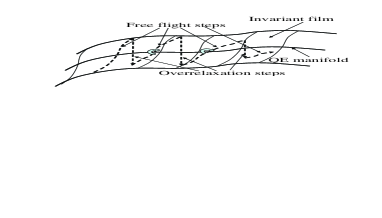
Figure 1: Directional instability: after several iterations the trajectory is not tangent to the invariant film with the required accuracy.

One could rely on the stability of this direction, but we fail to prove this in any general case. The directional instability changes the structure of dissipation terms: the accuracy decreases to the first-order in time step $h$ and significant fluctuations of the Prandtl number and viscosity, etc. may occur. This carries a danger even without blow-ups; one could conceivably be relying on nonreliable computational results.

Direction of neutral stability.

Further, there exists a neutral stability of all described approximations that causes one-step oscillations: a small shift of $f$ in the direction of $\Delta_{f^{*}_{M}}$ does not relax back for $\beta=1$, and its relaxation is slow for $\beta\sim 1$ (for small viscosity). This effect is demonstrated for a chain of mirror reflections in Fig. 2.

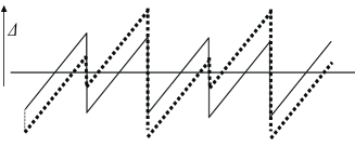
Figure 2: Neutral stability and one-step oscillations in a sequence of reflections. Bold dotted line – a perturbed motion, $\Delta$ – direction of neutral stability.

III.2 Dissipative recipes for stabilisation

Positivity rule.

There is a simple recipe for positivity preservation Rob_preprint ; Tosi06 : to substitute nonpositive $I_{0}^{\beta}(f)(\mbox{\boldmath$x$})$ by the closest nonnegative state that belongs to the straight line

$$\Bigr{\{}\lambda f(\mbox{\boldmath$x$})+(1-\lambda)\Pi^{*}(f(\mbox{\boldmath$x$}))|\>\lambda\in\mathbb{R}\Bigl{\}}$$ (37)

defined by the two points, $f(\mbox{\boldmath$x$})$ and its corresponding quasiequilibrium state. This operation is to be applied point-wise, at the points of the lattice where the positivity is violated. The coefficient $\lambda$ depends on $x$ too. Let us call this recipe the positivity rule (Fig. 3); it preserves positivity of populations and probabilities, but can affect the accuracy of approximation. The same rule is necessary for ELBGK (35) when a positive “mirror state” $\tilde{f}$ with the same entropy as $f$ does not exists on the straight line (37).

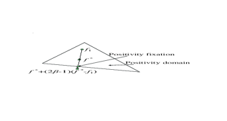
Figure 3: Positivity rule in action. The motions stops at the positivity boundary.

The positivity rule saves the existence of positive solutions, but affects dissipation because the result of the adjusted collision is closer to quasiequilibrium. There is a family of methods that modify collisions at some points by additional shift in the direction of quasiequilibrium. The positivity rule represents the minimal necessary modification. It is reasonable to always use this rule for LBM (as a “salvation rule”).

Ehrenfests’ regularisation.

To discuss methods with additional dissipation, the entropic approach is very convenient. Let entropy $S(f)$ be defined for each population vector $f=(f_{i})$ (below, we use the same letter $S$ for local-in-space entropy, and hope that the context will make this notation clear). We assume that the global entropy is a sum of local entropies for all sites. The local nonequilibrium entropy is

$$\Delta S(f)=S(f^{*})-S(f),$$ (38)

where $f^{*}$ is the corresponding local quasiequilibrium at the same point.

The Ehrenfests’ regularisation Rob_preprint ; Rob provides “entropy trimming”: we monitor local deviation of $f$ from the corresponding quasiequilibrium, and when $\Delta S(f,\mbox{\boldmath$x$})$ exceeds a pre-specified threshold value $\delta$, perform local Ehrenfests’ steps to the corresponding equilibrium. So that the Ehrenfests’ steps are not allowed to degrade the accuracy of LBGK it is pertinent to select the $k$ sites with highest $\Delta S>\delta$. The a posteriori estimates of added dissipation could easily be performed by analysis of entropy production in Ehrenfests’ steps. Numerical experiments show (see, e.g., Rob_preprint ; Rob and Sect. IV) that even a small number of such steps drastically improves stability.

To avoid the change of accuracy order “on average”, the number of sites with this step should be $\mathcal{O}(N\delta_{x}/L)$ where $N$ is the total number of sites, $\delta_{x}$ is the step of the space discretization and $L$ is the macroscopic characteristic length. But this rough estimate of accuracy in average might be destroyed by concentrations of Ehrenfests’ steps in the most nonequilibrium areas, for example, in boundary layers. In that case, instead of the total number of sites $N$ in the estimate $\mathcal{O}(N\delta_{x}/L)$ we should take the number of sites in a specific region . The effects of concentration could be easily analysed a posteriori.

Entropic steps for nonentropic equilibria.

If the approximate discrete equilibrium $f^{*}$ is nonentropic, we can use $\Delta S_{\rm K}(f)=-S_{\rm K}(f)$ instead of $\Delta S(f)$, where $S_{\rm K}$ is the Kullback entropy. This entropy,

$$S_{\rm K}(f)=-\sum_{i}f_{i}\ln\biggl{(}\frac{f_{i}}{f_{i}^{*}}\biggr{)},$$ (39)

gives the physically reasonable entropic distance from equilibrium, if the supposed continuum system has the classical BGS entropy. In thermodynamics, the Kullback entropy belongs to the family of Massieu–Planck–Kramers functions (canonical or grand canonical potentials). One can use (39) in the construction of Ehrenfests’ regularisation for any choice of discrete equilibrium.

We have introduced two procedures: the positivity rule and Ehrenfests’ regularisation. Both improve stability, reduce nonequilibrium entropy, and, hence, nonequilibrium fluxes. The proper context for discussion of such procedures are the flux-limiters in finite difference and finite volume methods. Here we refer to the classical flux-corrected transport (FCT) algorithm BorisBook1 that strictly maintains positivity, and to its further developments BookBoris2 ; Toro ; FCTMono .

Smooth limiters of nonequilibrium entropy.

The positivity rule and Ehrenfests’ regularisation provide rare, intense and localised corrections. Of course, it is easy and also computationally cheap to organize more gentle transformations with smooth shifts of higher nonequilibrium states to equilibrium. The following regularisation transformation distributes its action smoothly:

$$f\mapsto f^{*}+\phi(\Delta S(f))(f-f^{*}).$$ (40)

The choice of the function $\phi$ is highly ambiguous, for example, $\phi=1/(1+\alpha\Delta S^{k})$ for some $\alpha>0$, $k>0$. There are two significantly different choices: (i) ensemble-independent $\phi$ (i.e., the value of $\phi$ depends on the local value of $\Delta S$ only) and (ii) ensemble-dependent $\phi$, for example

$$\phi=\frac{1+(\Delta S/(\alpha{\rm E}(\Delta S)))^{k-1/2}}{1+(\Delta S/(\alpha{\rm E}(\Delta S)))^{k}}$$

where ${\rm E}(\Delta S)$ is the average value of $\Delta S$ in the computational area, $k\geq 1$ and $\alpha\gtrsim 1$. It is easy to select an ensemble-dependent $\phi$ with control of total additional dissipation.

ELBGK collisions as a smooth limiter.

On the basis on numerical tests, the authors of Tosi06 claim that the positivity rule provides the same results (in the sense of stability and absence/presence of spurious oscillations) as the ELBGK models, but ELBGK provides better accuracy.

For the formal definition of ELBGK (35) our tests do not support claims that ELBGK erases spurious oscillations (see Sect. IV below). Similar observations for Burgers equation has been reported in Bruce . We understand this situation in the following way. The entropic method consists of at least three components:

1. entropic quasiequilibrium defined by entropy maximisation;

2. entropy balanced collisions (35) that have to provide proper entropy balance;

3. a method for the solution of the transcendental equation $S(f)=S(\tilde{f})$ to find $\alpha=\alpha(f)$ in (35).

It appears that the first two items do not affect spurious oscillations at all, if we solve equation for $\alpha(f)$ with high accuracy. Additional viscosity could, potentially, be added by use of explicit analytic formulas for $\alpha(f)$. In order not to decrease entropy, the errors in these formulas always increase dissipation. This can be interpreted as a hidden transformation of the form (40), where the coefficients of $\phi$ also depend on $f^{*}$.

Compared to flux limiters, nonequilibrium entropy limiters have a great benefit: by summation of all entropy changes we can estimate the amount of additional dissipation the limiters introduce into the system.

III.3 Non-dissipative recipes for stabilisation

Microscopic error and macroscopic accuracy.

The invariant film $\mathfrak{q}$ is an invariant manifold for the free-flight transformation and for the temporal and entropic involutions. The linear involution $I_{0}$, as well as the ELBGK involution $I_{E}$, transforms a point $f\in\mathfrak{q}$ into a point $f^{\prime}$ with $f-f^{\prime}=\alpha\Delta_{\Pi^{*}(f)}+o(f-\Pi^{*}(f))$, i.e., the vector $f-f^{\prime}$ is “almost tangent” to $\mathfrak{q}$, and the distance from $f^{\prime}$ to $\mathfrak{q}$ has the order $\mathcal{O}(\|f-\Pi^{*}(f)\|^{2})$.

Hence, if the initial state belongs to $\mathfrak{q}$, and the distance from quasiequilibrium is small enough ($\sim\mathcal{O}(h)$), then during several steps the LBGK chain will remain near $\mathfrak{q}$ with deviation $\sim\mathcal{O}(h^{2})$. Moreover, because errors produced by collisions (deviations from $\mathfrak{q}$) have zero macroscopic projection, the corresponding macroscopic error in $M$ during several steps will remain of order $\mathcal{O}(h^{3})$.

To demonstrate this, suppose the error in $f$, $\delta f$, is of order $\mathcal{O}(h^{k})$, and $m(\delta f)=0$, then for smooth fields after a free-flight step an error of higher order appears in the macroscopic variables $M$: $m(\Theta_{h}(\delta f))=\mathcal{O}(h^{k+1})$, because $m(\Theta_{h}(\delta f))=m((\Theta_{h}-1)(\delta f))$ and $\Theta_{h}-1=\mathcal{O}(h)$. The last estimate requires smoothness.

This simple statement is useful for the error analysis we perform. We shall call it the lemma of higher macroscopic accuracy: a microscopic error of order $\mathcal{O}(h^{k})$ induces, after a time step $h$, a macroscopic error of order $\mathcal{O}(h^{k+1})$, if the field of macroscopic fluxes is sufficiently small (here, the microscopic error means the error that has zero macroscopic projection).

Restarts and approximation of $\Delta_{f^{*}_{M}}$.

The problem of nondissipative LBM stabilisation we interpret as a problem of appropriate restart from a point that is sufficiently close to the invariant film. If $h=\tau$ and collisions return the state to quasiequilibrium, then the state belongs to $\mathfrak{q}$ for all time with high accuracy. For $h\neq\tau$, formulas for restarting are also available: one can choose between (22) and, more flexibly, (23). Nevertheless, many questions remain. Firstly, what should one take for $\Delta_{f^{*}_{M}}$? This vector has a straightforward differential definition (10) (let us also recall that $\tau\Delta_{f^{*}_{M}}$ is the first Chapman–Enskog nonequilibrium correction to the distribution function (19)). But numerical differentiation could violate the exact-in-space free-flight transformation and local collisions. There exists a rather accurate central difference approximation of $\Delta_{f^{*}_{M}}$ on the basis of free-flight:

$$\Delta_{f^{*}_{M}}=\frac{1}{2}(\Delta^{+}_{f^{*}_{M}}+\Delta^{-}_{f^{*}_{M}})+\mathcal{O}(h^{2}),$$ (41)

where

$$\Delta^{+}_{f^{*}_{M}} =\frac{1}{h}(\Theta_{h}(f^{*}_{M})-\Pi^{*}(\Theta_{h}(f^{*}_{M}))),$$

$$\Delta^{-}_{f^{*}_{M}} =-\frac{1}{h}(\Theta_{-h}(f^{*}_{M})-\Pi^{*}(\Theta_{-h}(f^{*}_{M}))).$$

There are no errors of the first-order in (41). The forward ($\Delta^{+}_{f^{*}_{M}}$) and backward ($\Delta^{-}_{f^{*}_{M}}$) approximations are one order less accurate. The computation of $\Delta^{\pm}_{f^{*}_{M}}$ is of the same computational cost as an LBGK step, hence, if we use the restart formula (22) with central difference evaluation of $\Delta_{f^{*}_{M}}$ (41), then the computational cost increases three times (approximately). Non-locality of collisions (restart from the distribution $f^{s}_{M}$ (22) with a nonlocal expression for $\Delta_{f^{*}_{M}}$) spoils the main LBM idea of exact linear free-flight and local collisions: nonlocality is linear and exact, nonlinearity is local succi01 ). One might also consider the inclusion of other finite difference representations for $\Delta_{f^{*}_{M}}$ into explicit LBM schemes. The consequences of this combination should be investigated.

Coupled steps with quasiequilibrium ends.

The mean viscosity lemma allows us to combine different starting points in order to obtain the necessary macroscopic equations. From this lemma, it follows that the following construction of two coupled steps with restart from quasiequilibrium approximates the macroscopic equation (9) with second-order accuracy in time step $h$.

Let us take $f^{*}_{M}$ as the initial state with given $M$, then evolve the state by $\Theta_{h}$, apply the incomplete temporal involution $I_{T}^{\beta}$ (28), again evolve by $\Theta_{h}$, and finally project by $\Pi^{*}$ onto the quasiequilibrium manifold:

$$M\mapsto M^{\prime}=m(\Pi^{*}(\Theta_{h}(I_{T}^{\beta}(\Theta_{h}(f^{*}_{M}))))).$$ (42)

It follows from the restart formula (22) and the mean viscosity lemma that this step gives a second-order in time $h$ approximation to the shift in time $2h$ for (9) with $\tau=2(1-\beta)h$, $1/2\leq\beta\leq 1$. Now, let us replace $I_{T}^{\beta}$ by the much simpler transformation of LBGK collisions $I_{0}^{\beta}$ (33):

$$M\mapsto M^{\prime}=m(\Pi^{*}(\Theta_{h}(I_{0}^{\beta}(\Theta_{h}(f^{*}_{M}))))).$$ (43)

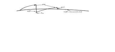
Figure 4: The scheme of coupled steps (43).

According to the lemma of higher macroscopic accuracy this step (Fig. 4) also gives a second-order in time $h$ approximation to the shift in time $2h$ for (9) with $\tau=2(1-\beta)h$, $1/2\leq\beta\leq 1$. The replacement of $I_{T}^{\beta}$ by $I_{0}^{\beta}$ introduces an error in $f$ that is of order $\mathcal{O}(h^{2})$, but both transformations conserve the value of macroscopic variables exactly. Hence (due to the lemma of higher macroscopic accuracy) the resulting error of coupled steps (43) in the macroscopic variables $M$ is of order $\mathcal{O}(h^{3})$. This means that the method has second-order accuracy.

Let us enumerate the macroscopic states in (43): $M_{0}=M$, $M_{1/2}=m(\Theta_{h}(f^{*}_{M}))$ and $M_{1}=M^{\prime}$. The shift from $M_{0}$ to $M_{1/2}$ approximates the shift in time $h$ for (9) with $\tau=h$. If we would like to model (9) with $\tau\ll h$, then $\tau=h$ means relatively very high viscosity. The step from $M_{1/2}$ to $M_{1}$ has to normalize viscosity to the requested small value (compare to antidiffusion in BorisBook1 ; BookBoris2 ). The antidiffusion problem necessarily appears in most CFD approaches to simulation flows with high-Reynolds numbers. Another famous example of such a problem is the filtering-defiltering problem in large eddy simulation (LES) Stolz . The antidiffusion in the coupled steps is produced by physical fluxes (by free-flight) and preserves positivity. The coupled step is a transformation $M_{0}\mapsto M_{1}$ and takes time $2h$. The middle point $M_{1/2}$ is an auxiliary state only.

Let us enumerate the microscopic states in (43): $f_{0}=f^{*}_{M}$, $f^{-}_{1/2}=\Theta_{h}(f^{*}_{M})$, $f^{0}_{1/2}=\Pi^{*}(f^{-}_{1/2})$, $\tilde{f}_{1/2}=I_{0}^{1}(f^{-}_{1/2})$, $f^{+}_{1/2}=f^{0}_{1/2}+(1-\beta)(\tilde{f}_{1/2}-f^{0}_{1/2})$, $f_{1}^{-}=\Theta_{h}(f^{+}_{1/2})$ $f_{1}=\Pi^{*}(f_{1}^{-})=f^{*}_{M_{1}}$, where $M_{1}=m(f_{1}^{-})$. Here, in the middle of the step, we have 4 points: a free-flight shift of the initial state ($f^{-}_{1/2}$), the corresponding quasiequilibrium ($f^{0}_{1/2}$), the mirror image ($\tilde{f}_{1/2}$) of the point $f^{-}_{1/2}$ with respect to the centre $f^{0}_{1/2}$, and the state ($f^{+}_{1/2}$) that is the image of $f^{-}_{1/2}$ after homothety with centre $f^{0}_{1/2}$ and coefficient $2\beta-1$.

For smooth fields, the time shift $\Theta_{h}$ returns $\tilde{f}_{1/2}$ to the quasiequilibrium manifold with possible error of order $\mathcal{O}(h^{2})$. For entropic equilibria, the nonequilibrium entropy of the state $\Theta_{h}(\tilde{f}_{1/2})$ is of order $\mathcal{O}(h^{4})$. This is an entropic estimate of the accuracy of antidiffusion: the nonequilibrium entropy of $\tilde{f}_{1/2}$ could be estimated from below as $C(M)h^{2}$, where $C(M)>0$ does not depend on $h$. The problem of antidiffusion can be stated as an implicit stepping problem: find a point $\tilde{f}$ such that

$$m(\tilde{f})=M,\quad(\Pi^{*}-1)(\Theta_{h}(\tilde{f}))=0.$$ (44)

This antidiffusion problem is a proper two-point boundary value problem. In a finite-dimensional space the first condition includes $N$ independent equations (where $N$ is the number of independent macroscopic variables), the second allows $N$ degrees of freedom, because the values of the macroscopic variables at that end are not fixed and $\Theta_{h}(\tilde{f})$ could be any point on the quasiequilibrium manifold). Shooting methods for the solution of this problem looks quite simple:

• Method A,

  $$\tilde{f}_{n+1}=\tilde{f}_{n}+\Pi^{*}(\Theta_{h}(\tilde{f}_{n}))-\Theta_{h}(\tilde{f}_{n}),$$ (45)

• Method B,

  $$\begin{split}\tilde{f}_{n+1}&=\Theta_{-h}(\Pi^{*}(\Theta_{h}(\tilde{f}_{n})))\\ &+f^{*}_{M}-\Pi^{*}(\Theta_{-h}(\Pi^{*}(\Theta_{h}(\tilde{f}_{n})))).\end{split}$$ (46)

Method A is: shoot from the previous approximation, $\tilde{f}_{n}$, by $\Theta_{h}$, project onto quasiequilibrium, $\Pi^{*}(\Theta_{h}(\tilde{f}_{n}))$, and then correction of $\tilde{f}_{n}$ by the final point displacement, $\Pi^{*}(\Theta_{h}(\tilde{f}_{n}))-\Theta_{h}(\tilde{f}_{n})$. The value of $M$ does not change, because $m(\Pi^{*}(\Theta_{h}(\tilde{f}_{n})))=m(\Theta_{h}(\tilde{f}_{n}))$.

Method B is: shoot from the previous approximation, $\tilde{f}_{n}$, by $\Theta_{h}$, project onto quasiequilibrium, shoot backwards by $\Theta_{-h}$, and then correction of $M$ using quasiequilibria (plus the quasiequilibrium with required value of $M$, and minus one with current value of $M$).

The initial approximation could be $\tilde{f}_{1/2}$, and $n$ here is the number of iteration. Due to the lemma of higher macroscopic accuracy, each iteration (45) or (46) increases the order of accuracy (see also the numerical test in Sec. IV).

The shooting method A (45) better meets the main LBM idea: each change of macroscopic variable is due to a free-flight step (because free-flight in LBM is exact), all other operations effect nonequilibrium component of the distribution only. The correction of $M$ in the shooting method B (46) violates this requirement.

The idea that all macroscopic changes are projections of free-flight plays, for the proposed LBM antidiffusion, the same role as the monotonicity condition for FCT BorisBook1 . In particular, free-flight never violates positivity.

If we a find solution $\tilde{f}$ to the antidiffusion problem with $M=M_{1/2}$, then we can take $f^{+}_{1/2}=f^{0}_{1/2}+(1-\beta)(\tilde{f}-f^{0}_{1/2})$, and $M_{1}=m(\Theta_{h}(f^{+}_{1/2}))$. But even exact solutions of (44) can cause stability problems: the entropy of $\tilde{f}$ could be less than the entropy of $f^{-}_{1/2}$, and blow-up could appear. A palliative solution is to perform an entropic step: to find $\alpha$ such that $S(f^{0}_{1/2}+\alpha(\tilde{f}-f^{0}_{1/2}))=S(f^{-}_{1/2})$, then use $f^{+}_{1/2}=f^{0}_{1/2}+(1-\beta)\alpha(\tilde{f}-f^{0}_{1/2})$. Even for nonentropic equilibria it is possible to use the Kullback entropy (39) for comparison of distributions with the same value of the macroscopic variables. Moreover, the quadratic approximation to (39) will not violate second-order accuracy, and does not require the solution of a transcendental equation.

The viscosity coefficient is proportional to $\tau$ and significantly depends on the chain construction: for the sequence (29) we have $\tau=(1-\beta)h/\beta$, and for the sequence of steps (43) $\tau=2(1-\beta)h$. For small $1-\beta$ the later gives around two times larger viscosity (and for realisation of the same viscosity we must take this into account).

How can the coupled steps method (43) fail? The method collects all the high order errors into dissipation. When the high-order errors accumulated in dissipation become compatible with the second-order terms, the observable viscosity significantly increases. In our numerical tests this catastrophe occurs when the hydrodynamic fields change significantly on 2-3 grid steps $\delta_{x}$ (the characteristic wave length $\lambda\sim 3\delta_{x}$). The catastrophe point is the same for the plain coupled steps (43) and for the methods with iterative corrections (45) or (46). The appropriate accuracy requires $\lambda\gtrsim 10\delta_{x}$. On the other hand, this method is a good solver for problems with shocks (in comparison with standard LBGK and ELBGK) and produces shock waves with very narrow fronts and almost without Gibbs effect. So, for sufficiently smooth fields it should demonstrate second-order accuracy, and in the vicinity of steep velocity derivatives it increases viscosity and produces artificial dissipation. Hence, this recipe is nondissipative in the main order only.

The main technical task in “stabilisation for accuracy” is to keep the system sufficiently close to the invariant film. Roughly speaking, we should correct the microscopic state $f$ in order to keep it close to the invariant film or to the tangent straight line $\{f^{*}_{M}+\lambda\Delta_{f^{*}_{M}}|\>\lambda\in\mathbb{R}\}$, where $M=m(f)$. But the general accuracy condition (23) gives much more freedom: the restart point should return to the invariant film in projections on the macroscopic variables and their fluxes only. A variant of such regularisation was de facto proposed and successfully tested in Latt . In the simplest realisation of such approaches a problem of “ghost” variables succi01 can arise: when we change the restart (22) to (23), neither moments, nor fluxes change. The difference is a “ghost” vector. At the next step, the introduced ghost component could affect fluxes, and at the following steps the coupling between ghost variables and macroscopic moments emerges. Additional relaxation times may be adjusted to suppress these nonhydrodynamic ghost variables Dellar .

Compromise between nonequilibrium memory and restart rules.

Formulas (22) and (23) prescribe a choice of restart states $f^{s}_{M}$. All memory from previous evolution is in the macroscopic state, $M$, only. There is no microscopic (or, alternatively, nonequilibrium) memory. Effects of nonequilibrium memory for LBM are not yet well studied. For LBGK with overrelaxation, these effects increase when $\beta$ approaches 1 because relaxation time decreases. We can formulate a hypothesis: observed sub-grid properties of various LBGK realisations and modifications for high-Reynolds number are due to nonequilibrium memory effects.

In order to find a compromise between the restart requirements (22), (23) and nonequilibrium memory existence we can propose to choose directions in concordance with (22), (23), where the nonequilibrium entropy field (38) does not change in the restart procedure. If after a free-flight step we have a distribution $f$ and find a corresponding restart state $f^{s}_{m(f)}$ due to a global rule, then for each grid point $x$ we can restart from a point $f^{*}_{m(f)}+\alpha(\mbox{\boldmath$x$})(f^{s}_{m(f)}-f^{*}_{m(f)})$, where $\alpha(\mbox{\boldmath$x$})>0$ is a solution of the constant local nonequilibrium entropy equation $S(f^{*}_{m(f)}(\mbox{\boldmath$x$})+\alpha(\mbox{\boldmath$x$})(f^{s}_{m(f)}(\mbox{\boldmath$x$})-f^{*}_{m(f)}(\mbox{\boldmath$x$})))=S(f(\mbox{\boldmath$x$}))$. This family of methods allows a minimal nonequilibrium memory – the memory about local entropic distance from quasiequilibrium.

IV Numerical experiment

IV.1 Velocities and equilibria

To conclude this paper we report two numerical experiments conducted to demonstrate the performance of some of the proposed LBM stabilisation recipes from Sect. III.

We choose velocity sets with entropic equilibria and an $H$-theorem in order to compare all methods in a uniform setting.

In 1D, we use a lattice with spacing and time step $h=1$ and a discrete velocity set $\{v_{1},v_{2},v_{3}\}:=\{0,-1,1\}$ so that the model consists of static, left- and right-moving populations only. The subscript $i$ denotes population (not lattice site number) and $f_{1}$, $f_{2}$ and $f_{3}$ denote the static, left- and right-moving populations, respectively. The entropy is $S=-H$, with

$$H=f_{1}\log(f_{1}/4)+f_{2}\log(f_{2})+f_{3}\log(f_{3}),$$

(see, e.g., karlin99 ) and, for this entropy, the local quasiequilibrium state $f^{*}$ is available explicitly:

$$f_{1}^{*} =\frac{2n}{3}\bigl{(}2-\sqrt{1+3u^{2}}\bigr{)},$$

$$f_{2}^{*} =\frac{n}{6}\bigl{(}(3u-1)+2\sqrt{1+3u^{2}}\bigr{)},$$

$$f_{3}^{*} =-\frac{n}{6}\bigl{(}(3u+1)-2\sqrt{1+3u^{2}}\bigr{)},$$

where

$$n:=\sum_{i}f_{i},\quad u:=\frac{1}{n}\sum_{i}v_{i}f_{i}.$$

In 2D, the realisation of LBGK that we use will employ a uniform $9$-speed square lattice with discrete velocities $\{v_{i}|\,i=0,1,\ldots 8\}$: $v_{0}=0$, $v_{i}=(\cos((i-1)\pi/{2}),\sin((i-1){\pi}/{2}))$ for $i=1,2,3,4$, $v_{i}=\sqrt{2}(\cos((i-5)\frac{\pi}{2}+\frac{\pi}{4}),\sin((i-5)\frac{\pi}{2}+\frac{\pi}{4}))$ for $i=5,6,7,8$. The numbering $f_{0}$, $f_{1},\dotsc,f_{8}$ are for the static, east, north, west, south, northeast, northwest, southwest and southeast-moving populations, respectively. As usual, the quasiequilibrium state, $f^{*}$, can be uniquely determined by maximising an entropy functional

$$S(f)=-\sum_{i}f_{i}\log{\Bigl{(}\frac{f_{i}}{W_{i}}\Bigr{)}},$$

subject to the constraints of conservation of mass and momentum ansumali03 :

$$f_{i}^{*}=nW_{i}\prod_{j=1}^{2}\Bigl{(}2-\sqrt{1+3u_{j}^{2}}\Bigr{)}\Biggl{(}\frac{2u_{j}+\sqrt{1+3u_{j}^{2}}}{1-u_{j}}\Biggr{)}^{v_{i,j}}.$$ (47)

Here, the lattice weights, $W_{i}$, are given lattice-specific constants: $W_{0}=4/9$, $W_{1,2,3,4}=1/9$ and $W_{5,6,7,8}=1/36$. The macroscopic variables are given by the expressions

$$n:=\sum_{i}f_{i},\quad(u_{1},u_{2}):=\frac{1}{n}\sum_{i}v_{i}f_{i}.$$

As we are advised in Sect. III, in all of the experiments, we implement the positivity rule.

IV.2 Shock tube

The $1$D shock tube for a compressible isothermal fluid is a standard benchmark test for hydrodynamic codes. Our computational domain will be the interval $[0,1]$ and we discretize this interval with $801$ uniformly spaced lattice sites. We choose the initial density ratio as 1:2 so that for $x\leq 400$ we set $n=1.0$ else we set $n=0.5$.

Basic test: LBGK, ELBGK and Coupled steps.

We will fix the kinematic viscosity of the fluid at $\nu=10^{-9}$ We should take $\beta=1/(2\nu+1)\approx 1-2\nu$ for LBGK and ELBGK (with or without the Ehrenfests’ regularisation). Whereas, for the coupled step regularisation, we should take $\beta=1-\nu$.

The governing equations for LBGK are

$$f_{i}(x+v_{i},t+1)\!=\!f_{i}^{*}(x,t)+(2\beta-1)(f_{i}^{*}(x,t)-\!f_{i}(x,t)).$$ (48)

For ELBGK (35) the governing equations are:

$$f_{i}(x+v_{i},t+1)=(1-\beta)f_{i}^{*}(x,t)+\beta\tilde{f}_{i}(x,t),$$ (49)

with $\tilde{f}=(1-\alpha)f+\alpha f^{*}$. As previously mentioned, the parameter, $\alpha$, is chosen to satisfy a constant entropy condition. This involves finding the nontrivial root of the equation

$$S((1-\alpha)f+\alpha f^{*})=S(f).$$ (50)

Inaccuracy in the solution of this equation can introduce artificial viscosity. To solve (50) numerically we employ a robust routine based on bisection. The root is solved to an accuracy of $10^{-15}$ and we always ensure that the returned value of $\alpha$ does not lead to a numerical entropy decrease. We stipulate that if, at some site, no nontrivial root of (50) exists we will employ the positivity rule instead.

The governing equations for the coupled step regularisation of LBGK alternates between classic LBGK steps and equilibration:

$$\begin{split}&f_{i}(x+v_{i},t+1)\\ &=\left\{\begin{aligned} &\!f_{i}^{*}(x,t),\qquad\text{$N_{\mathrm{step}}$ odd,}\\ &\!f_{i}^{*}(x,t)+(2\beta-1)(f_{i}^{*}(x,t)-f_{i}(x,t)),\,\text{$N_{\mathrm{step}}$ even,}\end{aligned}\right.\end{split}$$ (51)

where $N_{\mathrm{step}}$ is the cumulative total number of time steps taken in the simulation. For coupled steps, only the result of a couple of steps has clear physical meaning: this couple transforms $f_{i}^{*}(x,t)$ that appears at the beginning of an odd step to $f_{i}^{*}(x,t)$ that appears at the beginning of the next odd step.

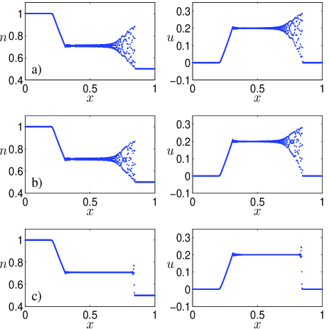
Figure 5: Density and velocity profile of the 1:2 isothermal shock tube simulation after $400$ time steps using (a) LBGK (48); (b) ELBGK (49); (e) coupled step regularisation (51); In this example, no negative population are produced by any of the methods so the positivity rule is redundant. For ELBGK in this example, (50) always has a nontrivial root.

As we can see, the choice between the two collision formulas LBGK (48) or ELBGK (49) does not affect spurious oscillation. But it should be mentioned that the entropic method consists of not only the collision formula, but, what is important, includes the provision of special choices of quasiequilibrium that could improve stability (see, e.g., Shyam2006 ). The coupled steps produce almost no spurious oscillations. This seems to be nice, but in such cases it is necessary to monitor the amount of artificial dissipation and to measure the viscosity provided by the method (see below).

Ehrenfests’ regularisation.

For the realisation of the Ehrenfests’ regularisation of LBGK, which is intended to keep states uniformly close to the quasiequilibrium manifold, we should monitor nonequilibrium entropy $\Delta S$ (38) at every lattice site throughout the simulation. If a pre-specified threshold value $\delta$ is exceeded, then an Ehrenfests’ step is taken at the corresponding site. Now, the governing equations become:

$$\begin{split}&f_{i}(x+v_{i},t+1)\\ &=\left\{\begin{aligned} &\!f_{i}^{*}(x,t)+(2\beta-1)(f_{i}^{*}(x,t)-f_{i}(x,t)),\,\text{$\Delta S\leq\delta$,}\\ &\!f_{i}^{*}(x,t),\qquad\text{otherwise,}\end{aligned}\right.\end{split}$$ (52)

Furthermore, so that the Ehrenfests’ steps are not allowed to degrade the accuracy of LBGK it is pertinent to select the $k$ sites with highest $\Delta S>\delta$. The a posteriori estimates of added dissipation could easily be performed by analysis of entropy production in Ehrenfests’ steps.

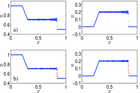
Figure 6: Density and velocity profile of the 1:2 isothermal shock tube simulation after $400$ time steps using Ehrenfests’ regularisation (52) with (a) $(k,\delta)=(4,10^{-3})$; (b) $(k,\delta)=(4,10^{-4})$. Sites where Ehrenfests’ steps are employed are indicated by crosses. Compare to Fig. 5a.

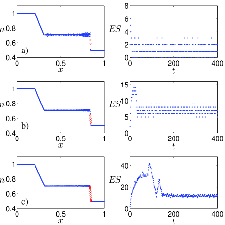
Figure 7: LBGK (48) regularised with Ehrenfests’ steps (52). Density profile of the 1:2 isothermal shock tube simulation and Ehrenfests’ steps histogram after 400 time steps using the tolerances (a) $(k,\delta)=(\infty,10^{-3})$; (b) $(k,\delta)=(\infty,10^{-4})$; (c) $(k,\delta)=(\infty,10^{-5})$. Sites where Ehrenfests’ steps are employed are indicated by crosses. Compare to Fig. 5a.

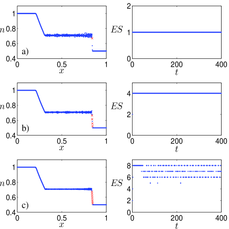
Figure 8: LBGK (48) regularised with Ehrenfests’ steps (52). Density profile of the 1:2 isothermal shock tube simulation and Ehrenfests’ steps histogram after 400 time steps using the tolerances (a) $(k,\delta)=(1,10^{-4})$; (b) $(k,\delta)=(4,10^{-4})$; (c) $(k,\delta)=(8,10^{-4})$. Sites where Ehrenfests’ steps are employed are indicated by crosses. Compare to Fig. 5a.

In the example in Fig. 6, we have considered fixed tolerances of $(k,\delta)=(4,10^{-3})$ and $(k,\delta)=(4,10^{-4})$ only. We reiterate that it is important for Ehrenfests’ steps to be employed at only a small share of sites. To illustrate, in Fig. 7 we have allowed $k$ to be unbounded and let $\delta$ vary. As $\delta$ decreases, the number of Ehrenfests’ steps quickly begins to grow (as shown in the accompanying histograms) and excessive and unnecessary smoothing is observed at the shock. The second-order accuracy of LBGK is corrupted. In Fig. 8, we have kept $\delta$ fixed at $\delta=10^{-4}$ and instead let $k$ vary. We observe that even small values of $k$ (e.g., $k=1$) dramatically improves the stability of LBGK.

IV.3 Accuracy of coupled steps

Coupled steps (43) give the simplest second–order accurate stabilization of LBGK. Stabilization is guaranteed by collection of all errors into dissipative terms. But this monotone collection of errors could increase the higher order terms in viscosity. Hence, it seems to be necessary to analyze not only order of errors, but their values too.

For accuracy analysis of coupled steps we are interested in the error in the antidiffusion step (44). We analyse one coupled step for $\beta=1$. The motion starts from a quasiequilibrium $f_{0}=f^{*}_{M}$, then a free-flight step $f^{-}_{1/2}=\Theta_{h}(f^{*}_{M})$, after that a simple reflection $\tilde{f}_{1/2}=I_{0}^{1}(f^{-}_{1/2})$ with respect to the quasiequilibrium centre $f^{0}_{1/2}=\Pi^{*}(f^{-}_{1/2})$, again a free-flight step, $f^{-}_{1}=\Theta_{h}(\tilde{f}_{1/2})$, and finally a projection onto quasiequilibrium, $f_{1}=\Pi^{*}(f^{-}_{1})$.

In the first of two accuracy tests, two types of errors are to be studied. The middle point displacement is

$$\delta_{\rm cs}=\|f^{0}_{1/2}-\Pi^{*}(\Theta_{-h}(f^{-}_{1}))\|/\|f_{0}-f^{0}_{1/2}\|.$$ (53)

To estimate nonequilibrity of the final point $f^{-}_{1}$ (i.e., additional dissipation introduced by last projection in the coupled step) we should compare the difference $f^{-}_{1}-f_{1}$ to the difference at the middle point $f^{-}_{1/2}-f^{0}_{1/2}$. Let us introduce

$$\sigma_{\rm cs}=\|f^{-}_{1}-f_{1}\|^{2}/\|f^{-}_{1/2}-f^{0}_{1/2}\|^{2}.$$ (54)

In our tests (Fig. 9) we use the $\ell_{2}$ norm.

We take the 1D 3-velocity model with entropic equilibria. Our computational domain will be the interval $[0,1]$ which we discretize with $1001$ uniformly spaced lattice sites. The initial condition is $n(x,0)=1+0.2\sin{(2\pi\omega x)}$, $u(x,0)=0.1\cos{(2\pi\omega x)}$ and we employ periodic boundary conditions. We compute a single coupled step for frequencies in the range $\omega=1,2,\dotsc,1000$ (Fig. 9).

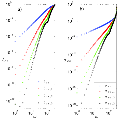
Figure 9: (a) The $\ell_{2}$ estimate of middle point displacement (53): for coupled steps (43) (diamonds), one (triangles), two (squares) and three (dots) shooting iterations (46); (b) The $\ell_{2}$ estimate of nonequilibrity of the final point (54): for coupled steps (43) (diamonds), one (triangles), two (stars) and three (squares) shooting iterations (46).

The solution $\tilde{f}$ to the antidiffusion problem could be corrected by the shooting iterations (45) and (46). The corresponding errors for method B (46) are also presented in Fig. 9. We use $\delta_{\rm{cs},i}$ and $\sigma_{\rm{cs},i}$, for $i=1,2,\dotsc$, to denote each subsequent shooting of (53) and (54), respectively.

We observe that the nonequilibrity estimate, $\sigma_{\rm cs}$, blows-up around the wavelength $1/\omega\sim 3\delta_{x}$. Simultaneously, the middle point displacement $\delta_{\rm cs}$ has value around unity at the same point. We do not plot the results for larger values of $\omega$ as the simulation has become meaningless and numerical aliasing will now decrease these errors. The same critical point is observed for each subsequent shooting as well. For this problem, the shooting procedure is demonstrated to be effective for wavelengths $1/\omega\lesssim 10\delta_{x}$.

For the second accuracy test we propose a simple test to measure the observable viscosity of a coupled step (and LBGK) simulation. We take the 2D isothermal 9-velocity model with entropic equilibria. Our computational domain will a square which we discretize with $(L+1)\times(L+1)$ uniformly spaced points and periodic boundary conditions. The initial condition is $n(x,y)=1$, $u_{1}(x,y)=0$ and $u_{2}(x,y)=u_{0}\sin(2\pi x/L)$, with $u_{0}=0.05$. The exact velocity solution to this problem is an exponential decay of the initial condition: $u_{1}(x,y,t)=0$, $u_{2}(x,y,t)=u_{0}\exp(-\lambda u_{0}t/(\mathrm{Re}L))\sin(2\pi x/L)$, where $\lambda$ is some constant and $\mathrm{Re}=\mathrm{Re}(\beta)=u_{0}L/\nu(\beta)$ is the Reynolds number of the flow. Here, $\nu=\nu(\beta)$ is the theoretical viscosity of the fluid: $\nu=1-\beta$ for the coupled steps (43) and $\nu=(1/\beta-1)/2$ for LBGK.

Now, we simulate the flow over $L/v_{0}$ time steps and measure the constant $\lambda$ from the numerical solution. We do this for both LBGK and the coupled steps (43) for $L=100$ and for $L=200$. The results (Fig. 10) show us that for coupled steps (and for LBGK to a much lesser extent) the observed viscosity is higher than the theoretical estimate, hence the observed $\mathrm{Re}$ is lower than the estimate. In particular, the lower-resolution ($L=100$) coupled steps simulation diverges from LBGK at around $\mathrm{Re}=500$. The two times higher-resolution ($L=200$) simulations are close to around $\mathrm{Re}=\mathcal{O}(1000)$, after which there begins to be a considerable increase in the observable viscosity (as explained within Sect. III.3).

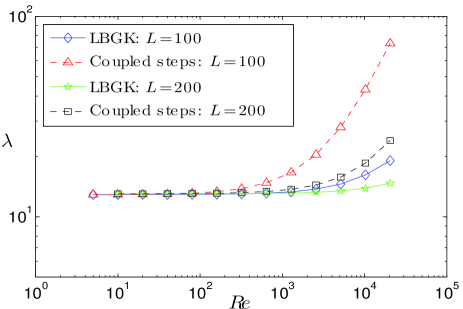
Figure 10: Numerically computed value of $\lambda$ versus Reynolds number for 2D accuracy test: LBGK with $L=100$ (diamonds); coupled steps (43) with $L=100$ (triangles); LBGK with $L=200$ (stars); coupled steps (43) with $L=200$ (squares).

IV.4 Flow around a square-cylinder

The unsteady flow around a square-cylinder has been widely experimentally investigated in the literature (see, e.g., vickery66 ; davis92 ; okajima82 ). The computational set up for the flow is as follows. A square-cylinder of side length $L$, initially at rest, is immersed in a constant flow in a rectangular channel of length $30L$ and height $25L$. The cylinder is place on the centre line in the $y$-direction resulting in a blockage ratio of $4$%. The centre of the cylinder is placed at a distance $10.5L$ from the inlet. The free-stream velocity is fixed at $(u_{\infty},v_{\infty})=(0.05,0)$ (in lattice units) for all simulations.

On the north and south channel walls a free-slip boundary condition is imposed (see, e.g., succi01 ). At the inlet, the inward pointing velocities are replaced with their quasiequilibrium values corresponding to the free-stream velocity. At the outlet, the inward pointing velocities are replaced with their associated quasiequilibrium values corresponding to the velocity and density of the penultimate row of the lattice.

Maxwell boundary condition.

The boundary condition on the cylinder that we prefer is the diffusive Maxwell boundary condition (see, e.g., cercignani75 ), which was first applied to LBM in ansumali02 . The essence of the condition is that populations reaching a boundary are reflected, proportional to equilibrium, such that mass-balance (in the bulk) and detail-balance are achieved. We will describe two possible realisations of the boundary condition – time-delayed and instantaneous reflection of equilibrated populations. In both instances, immediately prior to the advection of populations, only those populations pointing in to the fluid at a boundary site are updated. Boundary sites do not undergo the collisional step that the bulk of the sites are subjected to.

To illustrate, consider the situation of a wall, aligned with the lattice, moving with velocity $u_{\mathrm{wall}}$ and with outward pointing normal to the wall pointing in the positive $y$-direction (this is the situation on the north wall of the square-cylinder with $u_{\mathrm{wall}}=0$). The time-delayed reflection implementation of the diffusive Maxwell boundary condition at a boundary site $(x,y)$ on this wall consists of the update

$$f_{i}(x,y,t+1)=\alpha f^{*}_{i}(u_{\mathrm{wall}}),\qquad i=2,5,6,$$

with

$$\alpha=\frac{f_{4}(x,y,t)+f_{7}(x,y,t)+f_{8}(x,y,t)}{f^{*}_{2}(u_{\mathrm{wall}})+f^{*}_{5}(u_{\mathrm{wall}})+f^{*}_{6}(u_{\mathrm{wall}})}.$$

Whereas for the instantaneous reflection implementation we should use for $\alpha$:

$$\frac{f_{4}(x,y+1,t)\!+f_{7}(x+1,y+1,t)\!+f_{8}(x-1,y+1,t)}{f^{*}_{2}(u_{\mathrm{wall}})+f^{*}_{5}(u_{\mathrm{wall}})+f^{*}_{6}(u_{\mathrm{wall}})}.$$

Observe that, because density is a linear factor of the equilibria (47), the density of the wall is inconsequential in the boundary condition and can therefore be taken as unity for convenience.

We point out that, although both realisations agree in the continuum limit, the time-delayed implementation does not accomplish mass-balance. Therefore, instantaneous reflection is preferred and will be the implementation that we employ in the present example.

Finally, it is instructive to illustrate the situation for a boundary site $(x,y)$ on a corner of the square-cylinder, say the north-west corner. The (instantaneous reflection) update is then

$$f_{i}(x,y,t+1)=\beta f^{*}_{i}(u_{\mathrm{wall}}),\qquad i=2,3,5,6,7,$$

where

$$\beta = \beta_{0}/\beta_{\mathrm{wall}};$$

$$\beta_{0} = f_{1}(x-1,y,t)+f_{4}(x,y+1,t)$$

$$+f_{5}(x-1,y-1,t)+f_{7}(x+1,y+1,t)$$

$$+f_{8}(x-1,y+1,t);$$

$$\beta_{\mathrm{wall}} = f^{*}_{2}(u_{\mathrm{wall}})+f^{*}_{3}(u_{\mathrm{wall}})$$

$$+f^{*}_{5}(u_{\mathrm{wall}})+f^{*}_{6}(u_{\mathrm{wall}})+f^{*}_{7}(u_{\mathrm{wall}}).$$

Strouhal–Reynolds relationship.

As a test of the Ehrenfests’ regularisation (52), a series of simulations, all with characteristic length fixed at $L=20$, were conducted over a range of Reynolds numbers $\mathrm{Re}={Lu_{\infty}}/{\nu}$. The parameter pair $(k,\delta)$, which control the Ehrenfests’ steps tolerances, are fixed at $(L/2,10^{-3})$.

We are interested in computing the Strouhal–Reynolds relationship. The Strouhal number $\mathrm{St}$ is a dimensionless measure of the vortex shedding frequency in the wake of one side of the cylinder: $\mathrm{St}={Lf_{\omega}}/{u_{\infty}},$ where $f_{\omega}$ is the shedding frequency.

For our computational set up, the vortex shedding frequency is computed using the following algorithmic technique. Firstly, the $x$-component of velocity is recorded during the simulation over $t_{\mathrm{max}}=1250L/u_{\infty}$ time steps. The monitoring points is positioned at coordinates $(4L,-2L)$ (assuming the origin is at the centre of the cylinder). Next, the dominant frequency is extracted from the final $25$% of the signal using the discrete Fourier transform. The monitoring point is purposefully placed sufficiently downstream and away from the centre line so that only the influence of one side of the cylinder is recorded.

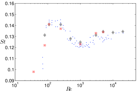
Figure 11: Variation of Strouhal number $\mathrm{St}$ as a function of Reynolds. Dots are Okajima’s experimental data okajima82 (the data has been digitally extracted from the original paper). Diamonds are the Ehrenfests’ regularisation of LBGK and the squares are the ELBGK simulation from ansumali04 .

The computed Strouhal–Reynolds relationship using the Ehrenfests’ regularisation of LBGK is shown in Fig. 11. The simulation compares well with Okajima’s data from wind tunnel and water tank experiment okajima82 . The present simulation extends previous LBM studies of this problem ansumali04 ; baskar04 which have been able to quantitively captured the relationship up to $\mathrm{Re}=\mathcal{O}(1000)$. Fig. 11 also shows the ELBGK simulation results from ansumali04 . Furthermore, the computational domain was fixed for all the present computations, with the smallest value of the kinematic viscosity attained being $\nu=5\times 10^{-5}$ at $\mathrm{Re}=20000$. It is worth mentioning that, for this characteristic length, LBGK exhibits numerical divergence at around $\mathrm{Re}=1000$. We estimate that, for the present set up, the computational domain would require at least $\mathcal{O}(10^{7})$ lattice sites for the kinematic viscosity to be large enough for LBGK to converge at $\mathrm{Re}=20000$. This is compared with $\mathcal{O}(10^{5})$ sites for the present simulation.

V Conclusions

In this paper, we have analysed LBM as a discrete dynamical system generated in distribution space by free-flight for time $\delta_{t}=h$ and involution (temporal or entropic, or just a standard LBGK reflection that approximates these involutions with second-order accuracy). Dissipation is produced by superposition of this involution with a homothety with centre in quasiequilibrium and coefficient $2\beta-1$.

Trajectories of this discrete dynamical system are projected on to the space of macroscopic variables, hydrodynamic fields, for example. The projection of a time step of the LBM dynamics in distribution space approximates a time shift for a macroscopic transport equation. We represent the general form of this equation (9), and provide necessary and sufficient conditions for this approximation to be of second-order accuracy in the time step $h$ (22), (23). This analysis includes conditions on the free-flight initial state, and does not depend on the particular collision model.

It is necessary to stress that for free-flight the space discretization is exact (introduces no errors), if the set of velocities consists of automorphisms of the grid.

It seems natural to discuss the LBM discrete dynamical system as an approximate solution to the kinetic equation, for example, to the BGK kinetics with a discrete velocity set (1). With this kinetic equation we introduce one more time scale, $\tau$. For $h>\tau$ (overrelaxation) the discrete LBM does not give a second-order in time step $h$ approximation to the continuous-in-time equation (1). This is obvious by comparison of “fast” direction relaxation times: it is $\tau$ for (1) and $h/(2(1-\beta))\sim h^{2}/\tau$ for discrete dynamics (see also Xiong ). Nevertheless, the “macroscopic shadow” of the discrete LBM with overrelaxation approximates the macroscopic transport equation with second-order in time step $h$ accuracy under the conditions (22) and (23).

We have presented the main mechanisms of observed LBM instabilities:

1. positivity loss due to high local deviation from quasiequilibrium;

2. appearance of neutral stability in some directions in the zero viscosity limit;

3. directional instability.

We have found three methods of stability preservation. Two of them, the positivity rule and the Ehrenfests’ regularisation, are “salvation” (or “SOS”) operations. They preserve the system from positivity loss or from the local blow-ups, but introduce artificial dissipation and it is necessary to control the number of sites where these steps are applied. In order to preserve the second-order of LBM accuracy, in average, at least, it is worthwhile to perform these steps on only a small number of sites; the number of sites should not be higher than $\mathcal{O}(N\delta_{x}/L)$, where $N$ is the total number of sites, $L$ is the macroscopic characteristic length and $\delta_{x}$ is the lattice step. Moreover, because these steps have a tendency to concentrate in the most nonequilibrium regions (boundary layers, shock layers, etc.), instead of the total number of sites one can use an estimate of the number of sites in this region.

The positivity rule and the Ehrenfests’ regularisation are members of a wide family of “nonequilibrium entropy limiters” that will play the same role, for LBM, as the flux limiters play for finite difference, finite volume and finite element methods. We have described this family and explained how to use entropy estimates for nonentropic equilibria. The great benefit of the LBM methods is that the dissipation added by limiters could easily be estimated a posteriori by summarising the entropy production.

Some practical recommendation for use of nonequilibrium entropy limiters are as follows:

• there exists a huge freedom in the construction of these limiters;

• for any important class of problems a specific optimal limiter could be found;

• one of the simplest and computationally cheapest nonequilibrium entropy limiters is the Ehrenfests’ regularisation with equilibration at $k$ sites with highest nonequilibrium entropy $\Delta S>\delta$ (the $(k,\delta)$-rule);

• the positivity rule should always be implemented.

The developed restart methods (Sec. III.3) (including coupled steps with quasiequilibrium ends) could provide second-order accuracy, but destroy the memory of LBM. This memory emerges in LBM with overrelaxation because of slow relaxation of nonequilibrium degrees of freedom (there is no such memory in the continuous-in-time kinetic equation with fast relaxation to the invariant slow Chapman–Enskog manifold). Now, we have no theory of this memory but can suggest a hypothesis that this memory is responsible for the LBM sub-grid properties. A compromise between memory and stability is proposed: one can use the directions of restart to precondition collisions, and keep the memory in the value of the field of local nonequilibrium entropy $\Delta S$ (or, for systems with nonentropic equilibria, in the value of the corresponding Kullback entropies (39)). Formally, this preconditioning generates a matrix collision model succi01 with a specific choice of matrix: in these models, the collision matrix is a superposition of projection (preconditioner), involution and homothety. A return from the simplest LBGK collision to matrix models has been intensively discussed recently in development of the multirelaxation time (MRT) models (for example, MRT ; Du , see also Rasin for matrix models for modelling of nonisotropic advection-diffusion problems, and Latt for regularisation matrix models for stabilisation at high-Reynolds numbers).

For second-order methods with overrelaxation, adequate second-order boundary conditions have to be developed. Without such conditions either additional dissipation or instabilities appear in boundary layers. The proposed schemes should now be put through the whole family of tests in order to find their place in the family of the LBM methods.

Recently, several approaches to stable LBM modelling of high-Reynolds number flows on coarse grids have been reported Geier ; Du ; KAAOS . Now it is necessary to understand better the mechanisms of the LBM sub-grid properties, and to create the theory that allows us to prove the accuracy of LBM for under-resolved turbulence modelling.

- (1) S. Ansumali, S. S. Chikatamarla, C. E. Frouzakis, and K. Boulouchos, Entropic lattice Boltzmann simulation of the flow past square-cylinder, Int. J. Mod. Phys. C 15, 435–445 (2004).
- (2) S. Ansumali and I. V. Karlin, Kinetic boundary conditions in the lattice Boltzmann method, Phys. Rev. E 66, 026311 (2002).
- (3) S. Ansumali, I. V. Karlin, and H. C. Ottinger, Minimal entropic kinetic models for hydrodynamics, Europhys. Let. 63, 798–804 (2003).
- (4) G. Baskar and V. Babu, Simulation of the unsteady flow around rectangular cylinders using the ISLB method, In: 34th AIAA Fluid Dynamics Conference and Exhibit, AIAA–2004–2651 (2004).
- (5) R. Benzi, S. Succi, and M. Vergassola, The lattice Boltzmann-equation – theory and applications, Phys. Rep. 222, 145–197 (1992).
- (6) P. L. Bhatnagar, E. P. Gross, and M. Krook, A model for collision processes in gases. I. Small amplitude processes in charged and neutral one-component systems, Phys. Rev. 94, 511–525 (1954).
- (7) B. M. Boghosian, P. J. Love, and J. Yepez, Entropic lattice Boltzmann model for Burgers equation, Phil. Trans. Roy. Soc. A 362, 1691–1702 (2004).
- (8) B. M. Boghosian, J. Yepez, P. V. Coveney, and A. J. Wager, Entropic lattice Boltzmann methods, R. Soc. Lond. Proc. Ser. A 457 (2007), 717–766 (2001).
- (9) D. L. Book, J. P. Boris, and K. Hain, Flux corrected transport II. Generalizations of the method, J. Comput. Phys. 18, 248-283 (1975).
- (10) J. P. Boris and D. L. Book, Flux corrected transport I. SHASTA, a fluid transport algorithm that works, J. Comput. Phys. 11, 38–69 (1973).
- (11) R. A. Brownlee, A. N. Gorban, and J. Levesley, Stabilisation of the lattice-Boltzmann method using the Ehrenfests’ coarse-graining, cond-mat/0605359 (2006).
- (12) R. A. Brownlee, A. N. Gorban, and J. Levesley, Stabilization of the lattice-Boltzmann method using the Ehrenfests’ coarse-graining, Phys. Rev. E 74, 037703 (2006).
- (13) R. A. Brownlee, A. N. Gorban, and J. Levesley, Stability and stabilization of the lattice Boltzmann method: Magic steps and salvation operations, cond-mat/0611444 (2006).
- (14) S. Chapman and T. Cowling, Mathematical theory of non-uniform gases (Third edition, Cambridge University Press, Cambridge, 1970).
- (15) C. Cercignani, Theory and Application of the Boltzmann Equation (Scottish Academic Press, Edinburgh, 1975).
- (16) S. Chen and G. D. Doolen, Lattice Boltzmann method for fluid flows, Annu. Rev. Fluid. Mech. 30, 329–364 (1998).
- (17) S. S. Chikatamarla and I. V. Karlin, Entropy and Galilean Invariance of Lattice Boltzmann Theories, Phys. Rev. Lett. 97, 190601 (2006)
- (18) A. J. Chorin, O. H. Hald, and R. Kupferman, Optimal prediction with memory, Physica D 166, 239–257 (2002).
- (19) R. W. Davis and E. F. Moore, A numerical study of vortex shedding from rectangles, J. Fluid Mech. 116, 475–506 (1982).
- (20) P. J. Dellar, Incompressible limits of lattice Boltzmann equations using multiple relaxation times, J. of Comput. Phys. 190, 351 -370 (2003).
- (21) R. Du, B. Shi, and X. Chen, Multi-relaxation-time lattice Boltzmann model for incompressible flow, Phys. Lett. A 359, 564- 572 (2006).
- (22) P. Ehrenfest and T. Ehrenfest, The conceptual foundations of the statistical approach in mechanics (Dover Publications Inc., New York, 1990).
- (23) M. Geier, A. Greiner, and J. G. Korvink, Cascaded digital lattice Boltzmann automata for high Reynolds number flow, Phys. Rev. E 73, 066705 (2006).
- (24) A. N. Gorban, Basic types of coarse-graining, In: A. N. Gorban, N. Kazantzis, I. G. Kevrekidis, H. C. Öttinger, and C. Theodoropoulos, editors, Model Reduction and Coarse-Graining Approaches for Multiscale Phenomena, 117–176 (Springer, Berlin-Heidelberg-New York, 2006) cond-mat/0602024.
- (25) A. N. Gorban, V. I. Bykov, and G. S. Yablonskii, Essays on Chemical relaxation (Novosibirsk, Nauka Publ., 1986).
- (26) A. N. Gorban and I. V. Karlin, General approach to constructing models of the Boltzmann equation, Physica A 206, 401–420 (1994).
- (27) A. N. Gorban and I. V. Karlin, Geometry of irreversibility: The film of nonequilibrium states, Preprint IHES/P/03/57 (Institut des Hautes Études Scientifiques, Bures-sur-Yvette, France, 2003), cond-mat/0308331.
- (28) A. N. Gorban and I. V. Karlin, Invariant manifolds for physical and chemical kinetics, vol. 660 of Lect. Notes Phys (Springer, Berlin-Heidelberg-New York, 2005).
- (29) A. N. Gorban, I. V. Karlin, Quasi-Equilibrium Closure Hierarchies for the Boltzmann Equation, Physica A 360, 325- 364 (2006).
- (30) A. N. Gorban, I. V. Karlin, H. C. Öttinger, and L. L. Tatarinova, Ehrenfest’s argument extended to a formalism of nonequilibrium thermodynamics, Phys. Rev. E 62, 066124 (2001).
- (31) H. Grad, On the kinetic theory of rarefied gases, Comm. Pure and Appl. Math. 2, 331–407 (1949).
- (32) X. He and L.-S. Luo, Theory of the lattice Boltzmann method: From the Boltzmann equation to the lattice Boltzmann equation, Phys. Rev. E 56, 6811–6817 (1997).
- (33) F. Higuera, S. Succi, and R. Benzi, Lattice gas – dynamics with enhanced collisions. Europhys. Lett. 9, 345–349 (1989).
- (34) C. W. Hirt, Heuristic stability theory for finite–difference equations, J. Comput. Phys. 2, 339–355 (1968).
- (35) D. d Humières, I. Ginzburg, M. Krafczyk, P. Lallemand, and L.-S. Luo, Multiplerelaxation – time lattice Boltzmann models in three-dimensions, Proc. Roy. Soc. London A 360, 437–451 (2002).
- (36) D. Jou, J. Casas-Vázquez, G. Lebon, Extended irreversible thermodynamics (Springer, Berlin, 1993).
- (37) M. Junk, A. Klar, and L. S. Luo, Asymptotic analysis of the lattice Boltzmann equation, J. Comput. Phys. 210, 676 -704 (2005).
- (38) I. V. Karlin, S. Ansumali, E. De Angelis, H. C. Öttinger, and S. Succi, Entropic Lattice Boltzmann Method for Large Scale Turbulence Simulation, cond-mat/0306003 (2003).
- (39) I. V. Karlin, S. Ansumali, C. E. Frouzakis, and S. S. Chikatamarla, Elements of the lattice Boltzmann method I: Linear advection equation, Commun. Comput. Phys., 1, 616–655 (2006).
- (40) I. V. Karlin, S. S. Chikatamarla, and S. Ansumali, Elements of the lattice Boltzmann method II: Kinetics and hydrodynamics in one dimension, Commun. Comput. Phys. 2, 196–238 (2007).
- (41) I. V. Karlin, A. Ferrante, and H. C. Öttinger, Perfect entropy functions of the lattice Boltzmann method, Europhys. Lett. 47, 182–188 (1999).
- (42) I. V. Karlin, A. N. Gorban, S. Succi, and V. Boffi, Maximum entropy principle for lattice kinetic equations, Phys. Rev. Lett. 81, 6–9 (1998).
- (43) D. Kuzmin, R. Lohner, and S. Turek (Eds.), Flux-Corrected Transport. Principles, Algorithms, and Applications, (Springer, Berlin–Heidelberg 2005).
- (44) J. Latt and B. Chopard, Lattice Boltzmann method with regularized pre-collision distribution function, Math. Comput. Simulat. 72, 165–168 (2006).
- (45) A. M. Lyapunov, The general problem of the stability of motion (Taylor & Francis, London, 1992).
- (46) A. Okajima, Strouhal numbers of rectangular cylinders, J. Fluid Mech. 123, 379–398 (1982).
- (47) I. Rasin, S. Succi and W. Miller, A multi-relaxation lattice kinetic method for passive scalar diffusion, J. Comput. Phys. 206, 453–462 (2005).
- (48) B. Robertson, Equations of motion in nonequilibrium statistical mechanics, Phys. Rev., 144, 151–161 (1966).
- (49) X. Shan, X-F. Yuan, and H. Chen, Kinetic theory representation of hydrodynamics: a way beyond the Navier Stokes equation, J. Fluid Mech. 550, 413- 441 (2006).
- (50) Y. I. Shokin The method of differential approximation (Springer, New York, 1983).
- (51) J. D. Sterling and S. Chen. Stability analysis of lattice Boltzmann methods, J. Comput. Phys. 123, 196–206 (1996).
- (52) S. Stolz and N. A. Adams, An approximate deconvolution procedure for large-eddy simulation, Phys. Fluids 11, 1699 (1999).
- (53) S. Succi, The lattice Boltzmann equation for fluid dynamics and beyond (Oxford University Press, New York, 2001).
- (54) S. Succi, I. V. Karlin, and H. Chen, Role of the H theorem in lattice Boltzmann hydrodynamic simulations. Rev. Mod. Phys. 74, 1203–1220 (2002).
- (55) E. F. Toro, Riemann solvers and numerical methods for fluid dynamics – a practical introduction (Springer, Berlin, 1997).
- (56) F. Tosi, S. Ubertini, S. Succi, H. Chen, and I. V. Karlin, Numerical stability of entropic versus positivity-enforcing lattice Boltzmann schemes, Math. Comput. Simulat. 72, 227–231 (2006).
- (57) B. J. Vickery, Fluctuating lift and drag on a long cylinder of square cross-section in a smooth and in a turbulent stream, J. Fluid Mech. 25, 481–494 (1966).
- (58) A. Xiong, Intrinsic instability of the lattice BGK model, Acta Mechanica Sinica (English Series) 18, 603–607 (2002).