Cotunneling through quantum dots coupled to magnetic leads: zero-bias anomaly for non-collinear magnetic configurations

Abstract

Cotunneling transport through quantum dots weakly coupled to non-collinearly magnetized leads is analyzed theoretically by means of the real-time diagrammatic technique. The electric current, dot occupations, and dot spin are calculated in the Coulomb blockade regime and for arbitrary magnetic configuration of the system. It is shown that an effective exchange field exerted on the dot by ferromagnetic leads can significantly modify the transport characteristics in non-collinear magnetic configurations, in particular the zero-bias anomaly found recently for antiparallel configuration. For asymmetric Anderson model, the exchange field gives rise to precession of the dot spin, which leads to a nonmonotonic dependence of the differential conductance and tunnel magnetoresistance on the angle between magnetic moments of the leads. An enhanced differential conductance and negative TMR are found for certain non-collinear configurations.

I Introduction

Transport through quantum dots coupled to ferromagnetic leads was a subject of extensive considerations in the last few years. wolf01 ; loss02 ; maekawa02 ; zutic04 Most of the works concerned theoretical description of spin-polarized transport in the strong coupling regime, where the Kondo physics emerges, surgueevPRB02 ; lopezPRL03 ; martinekPRL03 ; fransson05 ; utsumiPRB05 ; swirkowiczPRB06 ; eto_simon as well as in the weak coupling regime. When the energy of electrons of the source lead is larger than the corresponding charging energy of the dot, the current in the weak coupling regime flows through the system due to sequential (one by one) tunneling via discrete levels of the quantum dot. nato ; kouwenhoven97 On the other hand, if the applied voltage is below threshold for sequential tunneling, first-order transport is suppressed and the system is in the Coulomb blockade regime. In this transport regime the current can still be mediated by cotunneling processes, which involve correlated tunneling through virtual states of the quantum dot. odintsov ; nazarov ; kang

Sequential transport through a single-level quantum dot coupled to ferromagnetic leads was studied for both collinear bulka00 ; rudzinski01 and non-collinear exch_field ; rudzinski05 ; wetzels05 ; braun06 configurations of the electrodes’ magnetic moments. Spin-polarized transport in the cotunneling regime has been addressed mainly for collinear systems, weymannPRB05BR ; weymannPRB05 ; weymannPRB06 although some aspects of cotunneling through quantum dots coupled to non-collinearly magnetized leads have also been considered. pedersen05 ; braig05 ; weymannEPJ05 It has been shown weymannPRB05BR that the interplay of single-barrier and double-barrier cotunneling processes gives rise to zero-bias anomaly in the differential conductance $G$ when the leads’ magnetic moments are antiparallel. This, in turn, leads to the corresponding zero-bias anomaly in the tunnel magnetoresistance (TMR). Moreover, the even-odd electron number parity effect in TMR has also been found. weymannPRB05 On the other hand, if the dot hosts two orbital levels and the ground state is a triplet, zero-bias anomaly develops due to cotunneling through singlet and triplet states of the dot. weymannEPL06 Very recently, experimental realizations of quantum dots connected to ferromagnetic leads have also been presented. Such systems may be realized for example in granular structures, zhang05 carbon nanotubes, tsukagoshi99 ; zhao02 ; jensen05 ; sahoo05 single molecules, pasupathy04 magnetic tunnel junctions, fertAPL06 or single self-assembled InAs quantum dots. hamaya06

The main objective of this paper is to address the problem of spin-polarized cotunneling through a quantum dot coupled to ferromagnetic leads with non-collinearly aligned magnetic moments. The external magnetic field required to control magnetic configuration of the system is assumed to be small enough to neglect the Zeeman splitting of the dot level. When the system is in a non-collinear magnetic configuration, an effective exchange field can significantly modify the transport characteristics. exch_field We show that in the case of symmetric Anderson model, $\varepsilon=-U/2$, where $\varepsilon$ is the dot level energy and $U$ denotes the Coulomb correlation parameter, the zero-bias anomaly in differential conductance decreases monotonically with increasing deviation of magnetic configuration from the antiparallel alignment, and eventually vanishes in the parallel configuration. On the other hand, the effect of exchange field is most visible when the system is described by an asymmetric Anderson model, $\varepsilon\neq-U/2$, leading to a nontrivial variation of the differential conductance with the angle between magnetizations of the leads.

The anomalous behavior of the differential conductance leads to a related anomaly in TMR, weymannPRB05 which for arbitrarily aligned magnetizations of the leads can be defined as ${\rm TMR}=[I_{\rm P}-I(\varphi)]/I(\varphi)$, where $I_{\rm P}$ is the current flowing through the system in the parallel configuration $(\varphi=0)$ and $I(\varphi)$ is the current flowing in the non-collinear magnetic configuration (i.e. when there is an angle $\varphi$ between the leads’ magnetic moments). We show that the angular dependence of TMR strongly depends on the system parameters – in the case of asymmetric Anderson model TMR can become negative when the leads are aligned non-collinearly.

The paper is organized in the following way. In section II we present the model of single-level quantum dot coupled to non-collinearly magnetized leads. In section III we briefly describe the real-time diagrammatic technique used to calculate transport properties. We also present the perturbation expansion in the Coulomb blockade regime for the case of arbitrary magnetic configuration of the system. Numerical results followed by discussion are presented in section IV, while the conclusions are given in section V.

II Model

The schematic of the system considered is shown in Fig. 1. The system consists of a single-level quantum dot coupled to ferromagnetic leads, whose spin moments, $\mathbf{S}_{\rm L}$ and $\mathbf{S}_{\rm R}$ for left and right lead, form an arbitrary configuration. The magnetic configuration of the system is described by the angle $\varphi$ – when $\varphi=0$ ($\varphi=\pi$) the system is in the parallel (antiparallel) magnetic configuration, see Fig. 1.

The system is described by an Anderson-like Hamiltonian of the form

$$H=H_{\rm L}+H_{\rm R}+H_{\rm D}+H_{\rm T}\,,$$ (1)

where the first two components describe noninteracting itinerant electrons in the leads, $H_{\alpha}=\sum_{k\sigma}\varepsilon_{\alpha k\sigma}c_{\alpha k\sigma}^{\dagger}c_{\alpha k\sigma}$ for the left ($\alpha={\rm L}$) and right ($\alpha={\rm R}$) lead in the local reference frames. The energy of an electron with spin $\sigma$ and wave number $k$ in the lead $\alpha$ is denoted by $\varepsilon_{\alpha k\sigma}$, while $c_{\alpha k\sigma}^{\dagger}$ ($c_{\alpha k\sigma}$) is the corresponding creation (annihilation) operator. The dot is described by $H_{\rm D}$, which in the global reference frame can be expressed as $H_{\rm D}=\sum_{\sigma=\uparrow,\downarrow}\varepsilon d_{\sigma}^{\dagger}d_{\sigma}+Un_{\uparrow}n_{\downarrow}$, where $\varepsilon$ is the single-particle energy, while $d_{\sigma}^{\dagger}$ $(d_{\sigma})$ creates (destroys) a spin-$\sigma$ electron in the dot. The second term of the dot Hamiltonian describes the Coulomb interaction of two electrons of opposite spins residing in the dot, with $U$ denoting the corresponding correlation energy. For the system geometry shown in Fig. 1, the tunnel Hamiltonian is given by $H_{\rm T}=H_{\rm TL}+H_{\rm TR}$, with

$$H_{\rm TL}=\sum_{k}\left(T_{{\rm L}+}c_{{\rm L}k+}^{\dagger}d_{\uparrow}+T_{{\rm L}-}c_{{\rm L}k-}^{\dagger}d_{\downarrow}+{\rm h.c.}\right)\,,$$ (2)

while $H_{\rm TR}$ reads

$$H_{\rm TR}=\sum_{k}\left[\left(T_{{\rm R}+}c_{{\rm R}k+}^{\dagger}\cos\frac{\varphi}{2}-T_{{\rm R}-}c_{{\rm R}k-}^{\dagger}\sin\frac{\varphi}{2}\right)d_{\uparrow}\right.$$ (3)

$$\left.+\left(T_{{\rm R}+}c_{{\rm R}k+}^{\dagger}\sin\frac{\varphi}{2}+T_{{\rm R}-}a_{{\rm R}k-}^{\dagger}\cos\frac{\varphi}{2}\right)d_{\downarrow}+{\rm h.c.}\right]\,,$$

where $T_{\alpha\sigma}$ denotes the tunnel matrix elements between the dot states and the majority $(\sigma=+)$ or minority $(\sigma=-)$ electron states in the lead $\alpha$ when $\varphi=0$. The coupling of the dot to ferromagnetic leads in the case of collinear magnetic configuration is described by $\Gamma_{\alpha}^{\sigma}=2\pi|T_{\alpha\sigma}|^{2}\rho_{\alpha\sigma}$, where $\rho_{\alpha\sigma}$ is the density of states for the majority $(\sigma=+)$ and minority $(\sigma=-)$ electrons in the lead $\alpha$. It is convenient to express the coupling parameters in terms of spin polarization defined as $p_{\alpha}=(\Gamma_{\alpha}^{+}-\Gamma_{\alpha}^{-})/(\Gamma_{\alpha}^{+}+\Gamma_{\alpha}^{-})$. Thus, the coupling strength can be written as $\Gamma_{\alpha}^{\pm}=\Gamma_{\alpha}(1\pm p_{\alpha})$, where $\Gamma_{\alpha}=(\Gamma_{\alpha}^{+}+\Gamma_{\alpha}^{-})/2$. In the following, we assume that the couplings are symmetric, $\Gamma_{\rm L}=\Gamma_{\rm R}\equiv\Gamma/2$. As reported in Ref. kogan04, , in the weak coupling regime typical values of the dot-lead coupling strength $\Gamma$ are of the order of tens of $\mu$eV.

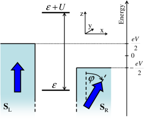
Figure 1: (color online) Schematic of a quantum dot coupled to ferromagnetic leads with non-collinearly aligned magnetizations. The net spin moments of the left $\mathbf{S}_{\rm L}$ and right $\mathbf{S}_{\rm R}$ lead form an angle $\varphi$. There is a symmetric bias voltage applied to the system.

We assume that the magnetic configuration of the system can be changed by applying a weak external magnetic field. The corresponding Zeeman energy is then very small and can be neglected. Thus, following previous theoretical calculations, weymannPRB05 we assume that the dot energy level is spin-degenerate. In the case of quantum dots, the magnetic fields that produce experimentally measurable effects are rather high, $\sim 10^{4}$ Oe. kogan04

III Method and Transport Equations

In order to calculate transport properties of the system we employ the real-time diagrammatic technique. diagrams ; koenigdiss This technique is based on a systematic perturbation expansion of the dot density matrix in the dot-lead coupling strength, which allows one to calculate transport characteristics order by order in tunneling processes. In the following, we address the problem of spin-polarized tunneling in the Coulomb blockade regime. In this transport regime the first-order (sequential) tunneling processes are exponentially suppressed due to the charging energy and the current is mediated by second- (cotunneling) or higher-order tunneling processes. odintsov ; nazarov ; kang

We note that although the approach based on the second-order perturbation theory and standard rate equation would lead to reasonable results for the Coulomb blockade regime and collinear magnetic configurations, it would be insufficient in the case of arbitrarily aligned magnetizations of the leads. This is because this approach does not allow for the effects of exchange field. On the other hand, the advantage of the real-time diagrammatic technique is that it takes into account the exchange field in a fully systematic way.

In our considerations we assume that the correlation parameter $U$ between two electrons in the dot is finite, which results in four dot states $|\chi\rangle$, with $\chi=0,\uparrow,\downarrow,{\rm d}$, respectively for the empty dot, singly occupied dot with spin-up or spin-down electron, and for two electrons in the dot. The density matrix of the dot involves then six elements,

$$\hat{\rho}_{\rm D}=\left(\begin{array}[]{cccc}P_{0}^{0}&0&0&0\\ 0&P_{\uparrow}^{\uparrow}&P_{\downarrow}^{\uparrow}&0\\ 0&P^{\downarrow}_{\uparrow}&P_{\downarrow}^{\downarrow}&0\\ 0&0&0&P_{\rm d}^{\rm d}\\ \end{array}\right).$$ (4)

The diagonal elements of the density matrix correspond to the respective occupation probabilities, while the off-diagonal elements $P_{\uparrow}^{\downarrow}$ and $P_{\downarrow}^{\uparrow}$ describe the dot spin $\vec{S}$, with $S_{x}={\rm Re}P_{\downarrow}^{\uparrow}$, $S_{y}={\rm Im}P_{\downarrow}^{\uparrow}$, and $S_{z}=\left(P_{\uparrow}^{\uparrow}-P_{\downarrow}^{\downarrow}\right)/2$. The time evolution of the dot density matrix is described by the Dyson equation, which can be transformed into a master-like equation. The master equation allows one to determine the elements of the density matrix. In the steady state and for spin-degenerate dot level it can be written as diagrams ; koenigdiss

$$0=\sum_{\chi_{1}^{\prime},\chi_{2}^{\prime}}P_{\chi^{\prime}_{2}}^{\chi^{\prime}_{1}}\Sigma_{\chi_{2}^{\prime}\chi_{2}}^{\chi_{1}^{\prime}\chi_{1}}\,,$$ (5)

where $\Sigma_{\chi_{2}^{\prime}\chi_{2}}^{\chi_{1}^{\prime}\chi_{1}}$ is the irreducible self-energy corresponding to transition forward in time from state $|\chi_{1}^{\prime}\rangle$ to $|\chi_{1}\rangle$ and then backward in time from state $|\chi_{2}\rangle$ to $|\chi_{2}^{\prime}\rangle$.

III.1 Dot occupations and spin

We consider transport in the Coulomb blockade regime, $|\varepsilon|,|\varepsilon+U|\gg\Gamma,k_{\rm B}T$, and when the dot is singly occupied, $\varepsilon<0<\varepsilon+U$. In order to calculate the dot occupations and spin, we expand the self-energies, ${\Sigma_{\chi_{2}^{\prime}\chi_{2}}^{\chi_{1}^{\prime}\chi_{1}}}=\sum_{j=1}{\Sigma_{\chi_{2}^{\prime}\chi_{2}}^{\chi_{1}^{\prime}\chi_{1}}}^{(j)}$, and density matrix elements, ${P_{\chi_{2}}^{\chi_{1}}}=\sum_{j=0}{P_{\chi_{2}}^{\chi_{1}}}^{(j)}$, order by order in tunneling processes. As a consequence, the master equation in the first order is given by

$$0=\sum_{\chi_{1}^{\prime},\chi_{2}^{\prime}}{P_{\chi^{\prime}_{2}}^{\chi^{\prime}_{1}}}^{(0)}{\Sigma_{\chi_{2}^{\prime}\chi_{2}}^{\chi_{1}^{\prime}\chi_{1}}}^{(1)}\,,$$ (6)

whereas the second-order master equation reads

$$0=\sum_{\chi_{1}^{\prime},\chi_{2}^{\prime}}{P_{\chi^{\prime}_{2}}^{\chi^{\prime}_{1}}}^{(0)}{\Sigma_{\chi_{2}^{\prime}\chi_{2}}^{\chi_{1}^{\prime}\chi_{1}}}^{(2)}+{P_{\chi^{\prime}_{2}}^{\chi^{\prime}_{1}}}^{(1)}{\Sigma_{\chi_{2}^{\prime}\chi_{2}}^{\chi_{1}^{\prime}\chi_{1}}}^{(1)}\,.$$ (7)

From the above equations and using the normalization, $\sum_{\chi}{P_{\chi}^{\chi}}^{(j)}=\delta_{j,0}$, one can find the density matrix elements in the zeroth and first order. Thus, the key point is to calculate the first- and second-order self-energies. This can be done with the aid of the following rules in the energy space:

1. Draw all topologically different diagrams with fixed time ordering and position of vertices. Connect the vertices by tunneling lines. Assign the energies of respective quantum dot states to the propagators and a frequency $\omega$ to each tunneling line.

2. Tunneling lines acquire arrows indicating whether an electron leaves or enters the dot. For tunneling lines changing the spin from $\sigma$ to $\sigma^{\prime}$ assign $\gamma^{+\sigma\sigma^{\prime}}_{\alpha}(\omega)$ $[\gamma^{-\sigma\sigma^{\prime}}_{\alpha}(\omega)]$ if the tunneling line goes backward (forward) with respect to the Keldysh contour and electron tunnels between the lead $\alpha$ and the dot.

3. For each time interval on the real axis limited by two adjacent vertices assign a resolvent $1/(\Delta E+i0^{+})$, with $\Delta E$ being the difference of all energies going from right minus all energies going from left.

4. Each diagram gets a prefactor $(-1)^{\gamma}$, with $\gamma$ being the number of internal vertices lying on the backward propagator plus the number of crossings of the tunneling lines, plus the number of vertices connecting state $|\rm d\rangle$ with state $|\downarrow\rangle$.

5. Integrate over all frequencies and sum up over the reservoirs.

The factor $\gamma^{\pm\sigma\sigma^{\prime}}_{\alpha}(\omega)$ is defined as, $\gamma^{\pm\sigma\sigma^{\prime}}_{\alpha}(\omega)=\Gamma^{\sigma\sigma^{\prime}}_{\alpha}f^{\pm}(\omega-\mu_{\alpha})$, with

$$\Gamma^{\uparrow\downarrow}_{\rm R} = \frac{1}{4\pi}\sin\varphi\left(\Gamma_{\rm R}^{+}-\Gamma_{\rm R}^{-}\right)\,,$$ (8)

$$\Gamma^{\uparrow\uparrow}_{\rm R} = \frac{1}{2\pi}\left(\Gamma_{\rm R}^{+}\cos^{2}\frac{\varphi}{2}+\Gamma_{\rm R}^{-}\sin^{2}\frac{\varphi}{2}\right)\,,$$ (9)

$$\Gamma^{\downarrow\downarrow}_{\rm R} = \frac{1}{2\pi}\left(\Gamma_{\rm R}^{+}\sin^{2}\frac{\varphi}{2}+\Gamma_{\rm R}^{-}\cos^{2}\frac{\varphi}{2}\right)\,,$$ (10)

while $\Gamma^{\sigma\sigma^{\prime}}_{\rm L}$ is given by changing ${\rm R\leftrightarrow L}$ and setting $\varphi=0$. Here, $f^{+}$ is the Fermi-Dirac distribution function, and $f^{-}=1-f^{+}$. We note that for arbitrary SU(2) rotations $\Gamma^{\downarrow\uparrow}_{\alpha}=\left(\Gamma^{\uparrow\downarrow}_{\alpha}\right)^{\star}$, while for rotations around the $y$ axis (considered in this paper) $\Gamma^{\downarrow\uparrow}_{\alpha}=\Gamma^{\uparrow\downarrow}_{\alpha}$.

By using the above rules, we find some useful general relations for the self-energies which hold in the first and second order

$${\Sigma_{\chi\bar{\sigma}}^{\chi\sigma}}^{(j)}=-\left[{\Sigma^{\chi\bar{\sigma}}_{\chi\sigma}}^{(j)}\right]^{*}\,,$$ (11)

$${\Sigma_{\bar{\sigma}\chi}^{\sigma\chi}}^{(j)}=-\left[{\Sigma^{\bar{\sigma}\chi}_{\sigma\chi}}^{(j)}\right]^{*}\,,$$ (12)

with $\chi=0,\uparrow,\downarrow,{\rm d}$ and $j=1,2$. In addition,

$${\Sigma_{\bar{\sigma}\chi^{\prime}}^{\sigma\chi}}^{(j)}=-\left[{\Sigma^{\bar{\sigma}\chi^{\prime}}_{\sigma\chi}}^{(j)}\right]^{*}\,,$$ (13)

for $\chi,\chi^{\prime}=\sigma,\bar{\sigma}$ ($\chi\neq\chi^{\prime}$), and ${\Sigma_{\bar{\sigma}\sigma}^{\sigma\bar{\sigma}}}^{(1)}=0$, as transition between such states has to involve at least two tunneling lines. In general, the self-energies are complex. However, as we show in the following, in the case of the Coulomb blockade regime one only needs to determine the imaginary parts of the second-order self-energies. This considerably simplifies numerical calculations, since the self-energies can be determined analytically.

First of all, we note that in the Coulomb blockade regime the first-order self-energies associated with energetically forbidden transitions are exponentially small, i.e., ${\Sigma_{\sigma\chi}^{\sigma\chi}}^{(1)}=0$, for $\chi=0,\uparrow,\downarrow,{\rm d}$, and ${\Sigma_{\bar{\sigma}\chi}^{\sigma\chi}}^{(1)}=0$, for $\chi=0,{\rm d}$. Furthermore, one also has ${\rm Im}{\Sigma_{\sigma\sigma}^{\sigma\bar{\sigma}}}^{(1)}={\rm Im}{\Sigma_{\sigma\sigma}^{\bar{\sigma}\sigma}}^{(1)}={\rm Im}{\Sigma_{\sigma\sigma}^{\bar{\sigma}\bar{\sigma}}}^{(1)}=0$. As a consequence, from the first-order master equation, Eq. (6), one finds, ${P_{0}^{0}}^{(0)}={P_{\rm d}^{\rm d}}^{(0)}=0$, and $S_{y}^{(0)}=0$, whereas the occupations ${P_{\uparrow}^{\uparrow}}^{(0)}$, ${P_{\downarrow}^{\downarrow}}^{(0)}$, and $S_{x}^{(0)}$ are related by the equation

$${P_{\uparrow}^{\uparrow}}^{(0)}{\Sigma^{\uparrow\uparrow}_{\uparrow\downarrow}}^{(1)}+{P_{\downarrow}^{\downarrow}}^{(0)}{\Sigma^{\downarrow\uparrow}_{\downarrow\downarrow}}^{(1)}+S_{x}^{(0)}{\Sigma^{\uparrow\uparrow}_{\downarrow\downarrow}}^{(1)}=0\,.$$ (14)

This equation, however, cannot be solved, as it involves three unknown variables. To solve for ${P_{\uparrow}^{\uparrow}}^{(0)}$, ${P_{\downarrow}^{\downarrow}}^{(0)}$, and $S_{x}^{(0)}$, it is necessary to include the second-order processes. If the system is in a collinear configuration (either parallel or antiparallel) the first two self-energies vanish ${\Sigma^{\uparrow\uparrow}_{\uparrow\downarrow}}^{(1)}={\Sigma^{\downarrow\uparrow}_{\downarrow\downarrow}}^{(1)}=0$, and Eq. (14) yields $S_{x}^{(0)}=0$. It is also worth noting that the above equation describes the effect of an exchange field which is exerted by ferromagnetic leads with non-collinearly aligned magnetizations. exch_field This exchange field results mainly from the first-order processes. To realize the meaning of Eq. (14) we rewrite this equation in a more explicit form (see the formulas given in Appendix A)

$$2{S_{z}}^{(0)}\mathcal{B}_{\rm R}^{\uparrow\downarrow}={{S_{x}}^{(0)}}\left(\mathcal{B}_{\rm L}^{\uparrow\uparrow}+\mathcal{B}_{\rm R}^{\uparrow\uparrow}-\mathcal{B}_{\rm L}^{\downarrow\downarrow}-\mathcal{B}_{\rm R}^{\downarrow\downarrow}\right)\,,$$ (15)

where

$$\mathcal{B}^{\sigma\sigma^{\prime}}_{\alpha}=\Gamma^{\sigma\sigma^{\prime}}_{\alpha}{\rm Re}\left[\Psi\left(\frac{1}{2}+i\frac{\varepsilon-\mu_{\alpha}}{2\pi k_{\rm B}T}\right)\right.$$

$$\left.-\Psi\left(\frac{1}{2}+i\frac{\varepsilon+U-\mu_{\alpha}}{2\pi k_{\rm B}T}\right)\right]$$ (16)

describe the exchange field effects, with $\Psi$ denoting the digamma function. exch_field The exchange field results from the spin-dependent virtual processes between the dot and leads. The angular variation of the exchange field is mainly governed by $\mathcal{B}^{\uparrow\downarrow}_{\rm R}\sim p_{\rm R}\Gamma_{\rm R}\sin\varphi$ ($\mathcal{B}^{\uparrow\downarrow}_{\rm L}=0$ in the assumed coordinate system). We note that $\mathcal{B}^{\uparrow\downarrow}_{\rm R}$ vanishes for collinear magnetic configurations as well as for nonmagnetic leads. As follows from Eq. (15), the exchange field in the first order gives rise to the rotation of the dot spin in the $x-z$ plane. mu06 Furthermore, we note that it is a purely many-body effect, as the exchange field vanishes in the noninteracting case, $U=0$.

Taking into account the aforementioned results and remarks, one can set up the second-order master equation, Eq. (7), for the Coulomb blockade regime. From the master equation in the second-order one gets a set of equations which, together with Eq. (14), allows one to determine ${P_{\uparrow}^{\uparrow}}^{(0)}$ and ${P_{\downarrow}^{\downarrow}}^{(0)}$, ${P_{0}^{0}}^{(1)}$ and ${P_{\rm d}^{\rm d}}^{(1)}$, and also $S_{x}^{(0)}$ and $S_{y}^{(1)}$. The equations which enable full solution of the problem can be written in a matrix form as

$$\left(\begin{array}[]{cccccc}0&{\Sigma^{\uparrow\uparrow}_{\uparrow\downarrow}}^{(1)}&{\Sigma^{\downarrow\uparrow}_{\downarrow\downarrow}}^{(1)}&0&{\Sigma^{\uparrow\uparrow}_{\downarrow\downarrow}}^{(1)}&0\\ {\Sigma^{00}_{00}}^{(1)}&{\Sigma^{\uparrow 0}_{\uparrow 0}}^{(2)}&{\Sigma^{\downarrow 0}_{\downarrow 0}}^{(2)}&0&2i{\rm Im}{\Sigma^{\uparrow 0}_{\downarrow 0}}^{(2)}&0\\ {\Sigma^{0\uparrow}_{0\uparrow}}^{(1)}&{\Sigma^{\uparrow\uparrow}_{\uparrow\uparrow}}^{(2)}&{\Sigma^{\downarrow\uparrow}_{\downarrow\uparrow}}^{(2)}&{\Sigma^{\rm d\uparrow}_{\rm d\uparrow}}^{(1)}&2i{\rm Im}{\Sigma^{\uparrow\uparrow}_{\downarrow\uparrow}}^{(2)}&2i{\Sigma^{\uparrow\uparrow}_{\downarrow\uparrow}}^{(1)}\\ {\Sigma^{0\downarrow}_{0\downarrow}}^{(1)}&{\Sigma^{\uparrow\downarrow}_{\uparrow\downarrow}}^{(2)}&{\Sigma^{\downarrow\downarrow}_{\downarrow\downarrow}}^{(2)}&{\Sigma^{\rm d\downarrow}_{\rm d\downarrow}}^{(1)}&2i{\rm Im}{\Sigma^{\uparrow\downarrow}_{\downarrow\downarrow}}^{(2)}&2i{\Sigma^{\uparrow\downarrow}_{\downarrow\downarrow}}^{(1)}\\ {\Sigma^{0\uparrow}_{0\downarrow}}^{(1)}&i{\rm Im}{\Sigma^{\uparrow\uparrow}_{\uparrow\downarrow}}^{(2)}&i{\rm Im}{\Sigma^{\downarrow\uparrow}_{\downarrow\downarrow}}^{(2)}&{\Sigma^{\rm d\uparrow}_{\rm d\downarrow}}^{(1)}&i{\rm Im}\left[{\Sigma^{\downarrow\uparrow}_{\uparrow\downarrow}}^{(2)}+{\Sigma^{\uparrow\uparrow}_{\downarrow\downarrow}}^{(2)}\right]&i{\Sigma^{\uparrow\uparrow}_{\downarrow\downarrow}}^{(1)}\\ 0&\Gamma&\Gamma&0&0&0\\ \end{array}\right)\left(\begin{array}[]{c}{P_{0}^{0}}^{(1)}\\ {P_{\uparrow}^{\uparrow}}^{(0)}\\ {P_{\downarrow}^{\downarrow}}^{(0)}\\ {P_{\rm d}^{\rm d}}^{(1)}\\ S_{x}^{(0)}\\ S_{y}^{(1)}\end{array}\right)=\left(\begin{array}[]{c}0\\ 0\\ 0\\ 0\\ 0\\ \Gamma\\ \end{array}\right)\,,$$ (17)

where the last row is due to the normalization condition, ${P_{\uparrow}^{\uparrow}}^{(0)}+{P_{\downarrow}^{\downarrow}}^{(0)}=1$. Equation (17) involves only the imaginary parts of the second-order self-energies which can be calculated analytically. The formulas for the self-energies appearing in Eq. (17) and having at the ends the off-diagonal states are given in Appendix A.

From the second-order master equation one also obtains an additional equation which involves ${P_{\uparrow}^{\uparrow}}^{(1)}$, ${P_{\downarrow}^{\downarrow}}^{(1)}$, and $S_{x}^{(1)}$,

$$0 = {P_{\uparrow}^{\uparrow}}^{(0)}{\rm Re}{\Sigma^{\uparrow\uparrow}_{\uparrow\downarrow}}^{(2)}+{P_{\downarrow}^{\downarrow}}^{(0)}{\rm Re}{\Sigma^{\downarrow\uparrow}_{\downarrow\downarrow}}^{(2)}+S_{x}^{(0)}{\rm Re}{\Sigma^{\uparrow\uparrow}_{\downarrow\downarrow}}^{(2)}$$ (18)

$$+{P_{\uparrow}^{\uparrow}}^{(1)}{\Sigma^{\uparrow\uparrow}_{\uparrow\downarrow}}^{(1)}+{P_{\downarrow}^{\downarrow}}^{(1)}{\Sigma^{\downarrow\uparrow}_{\downarrow\downarrow}}^{(1)}+S_{x}^{(1)}{\Sigma^{\uparrow\uparrow}_{\downarrow\downarrow}}^{(1)}\,.$$

This equation is analogous to Eq. (14) in the first order. To solve it for ${P_{\uparrow}^{\uparrow}}^{(1)}$, ${P_{\downarrow}^{\downarrow}}^{(1)}$, and $S_{x}^{(1)}$ one would need to include the higher-order (third-order) diagrams. In the case of collinear magnetic configurations, ${\Sigma^{\uparrow\uparrow}_{\uparrow\downarrow}}^{(j)}={\Sigma^{\downarrow\uparrow}_{\downarrow\downarrow}}^{(j)}=0$ for $j=1,2$, and from Eq. (18) one finds $S_{x}^{(1)}=0$, while $S_{x}^{(0)}=0$ from the first order master equation. Thus, if the magnetizations of the leads are aligned collinearly, Eq. (17) reduces to the one presented in Ref. weymannPRB05, .

III.2 Green’s functions and the current

The current flowing through the system can be expressed in terms of the Green’s functions as meir92

$$I = \frac{ie}{2h}\int d\omega{\rm Tr}\left\{\left[\mathbf{\Gamma}_{\rm L}f_{\rm L}^{+}(\omega)-\mathbf{\Gamma}_{\rm R}f_{\rm R}^{+}(\omega)\right]\right.$$ (19)

$$\left.\times\left[\mathbf{G^{>}}(\omega)-\mathbf{G^{<}}(\omega)\right]+\left(\mathbf{\Gamma}_{\rm L}-\mathbf{\Gamma}_{\rm R}\right)\mathbf{G^{<}}(\omega)\right\}\,,$$

with

$$\mathbf{G^{\lessgtr}}=\left(\begin{array}[]{cc}G_{\uparrow\uparrow}^{\lessgtr}&G_{\uparrow\downarrow}^{\lessgtr}\\ G_{\downarrow\uparrow}^{\lessgtr}&G_{\downarrow\downarrow}^{\lessgtr}\end{array}\right)\,.$$ (20)

The coupling matrices are given by

$$\mathbf{\Gamma}_{\rm R}=\Gamma_{\rm R}\left(\begin{array}[]{cc}1+p_{\rm R}\cos\varphi&p_{\rm R}\sin\varphi\\ p_{\rm R}\sin\varphi&1-p_{\rm R}\cos\varphi\end{array}\right)\,,$$ (21)

for the right lead and

$$\mathbf{\Gamma}_{\rm L}=\Gamma_{\rm L}\left(\begin{array}[]{cc}1+p_{\rm L}&0\\ 0&1-p_{\rm L}\end{array}\right)\,,$$ (22)

for the left lead. The Green’s functions $G_{\sigma\sigma^{\prime}}^{\lessgtr}(\omega)$ are defined as Fourier transforms of

$$G_{\sigma\sigma^{\prime}}^{<}(t) = i\langle d_{\sigma^{\prime}}^{\dagger}(0)d_{\sigma}(t)\rangle\,,$$ (23)

$$G_{\sigma\sigma^{\prime}}^{>}(t) = -i\langle d_{\sigma}(t)d_{\sigma^{\prime}}^{\dagger}(0)\rangle\,.$$ (24)

In order to calculate the current in each order we expand the Green’s functions systematically in the coupling strength $\Gamma$ koenigdiss

$$G_{\sigma\sigma^{\prime}}^{\lessgtr}=\sum_{m=0}^{\infty}G_{\sigma\sigma^{\prime}}^{\lessgtr(m)}=\sum_{m=0}^{\infty}\sum_{n=0}^{m}G_{\sigma\sigma^{\prime}}^{\lessgtr(n,m-n)}\,.$$ (25)

Thus, for the first order one has $G_{\sigma\sigma^{\prime}}^{\lessgtr(0)}=G_{\sigma\sigma^{\prime}}^{\lessgtr(0,0)}$, whereas in the second order with respect to $\Gamma$ the Green’s functions are given by $G_{\sigma\sigma^{\prime}}^{\lessgtr(1)}=G_{\sigma\sigma^{\prime}}^{\lessgtr(0,1)}+G_{\sigma\sigma^{\prime}}^{\lessgtr(1,0)}$. In the case of Coulomb blockade regime, the first-order current is exponentially suppressed and the dominant contribution comes from the second-order processes. Therefore, one only needs to calculate the Green’s functions in the second order. This can be done using the following rules in the energy space:

1. Assign the corresponding external and, in higher orders, internal vertices to a bare Keldysh contour. Connect the external vertices by a virtual line and the internal vertices by tunneling lines. Assign the energies of the respective quantum dot states to the propagators and a frequency $\omega$ to each tunneling line and the virtual line. Multiply the diagram with an element of the reduced density matrix corresponding to the initial state.

2. See rule (2) in calculation of self-energies.

3. See rule (3) in calculation of self-energies.

4. See rule (4) in calculation of self-energies.

5. Integrate over all frequencies except for the virtual line and sum up over the reservoirs.

For the lesser Green’s function an additional minus sign appears, which is due to reversed direction of the virtual line. The formulas for the Green’s functions in the Coulomb blockade regime are given in Appendix B.

IV Results and discussion

In the following we discuss numerical results on electronic transport through a single-level quantum dot coupled to non-collinearly magnetized leads. We first present the results for a symmetric Anderson model, $\varepsilon=-U/2$, then we proceed with the discussion of an asymmetric Anderson model, $\varepsilon\neq-U/2$. If $\varepsilon=-U/2$, the exchange field vanishes and both differential conductance and TMR change monotonically when going from parallel to antiparallel magnetic configurations. However, for $\varepsilon\neq-U/2$, the effects of exchange field become important and lead to nontrivial behavior of transport characteristics. The symmetric and asymmetric Anderson models can be realized experimentally by applying a gate voltage to the dot. With the gate voltage, one can continuously shift position of the dot level (while $U$ is unaffected) and thus study the cross-over from symmetric to asymmetric models.

IV.1 Symmetric Anderson model

Figure 2: (color online) (a) Differential conductance $G=dI/dV$ as a function of the bias voltage $V$ and the angle $\varphi$ for the symmetric Anderson model. The parameters are: $k_{\rm B}T=0.5\Gamma$, $\varepsilon=-15\Gamma$, $U=30\Gamma$, and $p_{\rm L}=p_{\rm R}\equiv p=0.5$. Part (b) shows the bias dependence of differential conductance for several angles.

The differential conductance $G$ as a function of the bias voltage and the angle $\varphi$ is shown in Fig. 2(a), while Fig. 2(b) displays the bias dependence of $G$ for several values of $\varphi$. In the collinear, i.e. parallel and antiparallel magnetic configurations we recover the earlier results, weymannPRB05BR with the zero-bias anomaly present in the antiparallel configuration and a parabolic dependence of $G$ on bias voltage for the parallel configuration. Now, we find a monotonic variation of the anomaly with the angle between leads’ magnetic moments. When the angle increases from zero to $\pi$, the anomaly emerges at small values of $\varphi$ and its relative height increases with increasing angle, reaching a maximum value at $\varphi=\pi$. The anomaly results from the interplay of nonequilibrium spin accumulation in the dot and the competition between the single-barrier and double-barrier cotunneling processes. The physical mechanism of this anomalous behavior was discussed in detail in Ref. [weymannPRB05BR, ], therefore, we will not describe it here. Instead, we will focus on its variation with the angle between magnetic moments of the leads and on the difference between symmetric and asymmetric Anderson models.

In the linear response regime and for symmetric Anderson model the exchange field, Eq. (III.1), is negligible and the average dot spin tends to zero. It is therefore relatively easy to find an approximate formula for the differential conductance. For $\varepsilon=-U/2$, $p_{\rm L}=p_{\rm R}\equiv p$, and at low temperatures, the angular dependence of the linear conductance is given by

$$G=\frac{e^{2}\Gamma^{2}}{2h\varepsilon^{2}}\left[3-p^{2}\left(1+2\sin^{2}\frac{\varphi}{2}\right)\right]\,.$$ (26)

The variation of $G$ with $\varphi$ at low bias is thus characterized by the factor $1+2\sin^{2}(\varphi/2)$, which leads to maximum (minimum) conductance in the parallel (antiparallel) magnetic configuration. Such behavior is typical of a normal spin-valve effect.

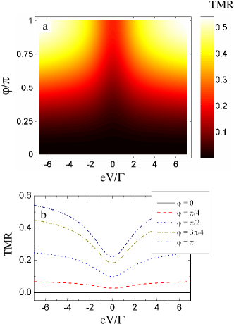
Figure 3: (color online) (a) Tunnel magnetoresistance as a function of the bias voltage $V$ and the angle $\varphi$ for the symmetric Anderson model. The parameters the same as in Fig. 2. Part (b) shows the TMR as a function of the bias voltage for several values of $\varphi$.

The TMR ratio, defined in the introduction, is shown in Fig. 3, where part (a) displays the angular and bias dependence, while part (b) shows the bias dependence of TMR for several values of the angle $\varphi$. The zero-bias anomaly in the differential conductance (see Fig. 2) leads to the corresponding anomaly (dip) in the TMR at small bias voltages. For collinear configurations we recover again the results presented in Ref. [weymannPRB05, ]. The dip in TMR decreases when magnetic configuration departs from the antiparallel one, and eventually disappears in the parallel configuration. The variation of TMR with the angle is monotonic, similarly as the angular variation of the differential conductance.

With the same assumptions as those made when deriving Eq. (26), one can approximate the dependence of TMR on the angle $\varphi$ at zero bias by

$${\rm TMR}=\frac{2p^{2}\sin^{2}\frac{\varphi}{2}}{3-p^{2}\left(1+2\sin^{2}\frac{\varphi}{2}\right)}\,.$$ (27)

Now, the angular dependence of TMR is governed by $\sin^{2}(\varphi/2)$, which gives maximum TMR in the antiparallel configuration and zero TMR in the parallel one.

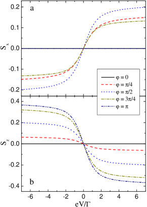
Figure 4: (color online) The $S_{x}$ (a) and $S_{z}$ (b) components of the dot spin as a function of the bias voltage for several values of the angle $\varphi$ as indicated in the figure. The other parameters are the same as in Fig. 2. In part (a) the curves for $\varphi=0$ and $\varphi=\pi$ coincide.

In Fig. 4 we show the average components $S_{x}$ and $S_{z}$ of the dot spin as a function of the bias voltage, calculated for several values of the angle $\varphi$. As one can see, $S_{x}=0$ and $S_{z}=0$ in the parallel magnetic configuration ($\varphi=0$), while in the antiparallel configuration ($\varphi=\pi$) $S_{x}=0$ whereas $S_{z}$ is finite. The $y$ component of the dot spin vanishes, $S_{y}=0$, irrespective of magnetic configuration of the system, so it is not shown in Fig. 4. As a consequence, up to the second order in tunneling processes, the average dot spin is in the $x-z$ plane, which is a characteristic feature of the symmetric Anderson model, $\varepsilon=-U/2$. In other words, there is no precession of the spin out of the $x-z$ plane, that is out of the plane formed by magnetic moments of the two electrodes. This is due to the cancellation of different contributions to the exchange field in the case of symmetric Anderson model. The absence of exchange field is responsible for the monotonic angular variation of both the differential conductance and TMR, discussed above, and also for vanishing of $S_{y}$ component of the dot spin.

IV.2 Asymmetric Anderson model

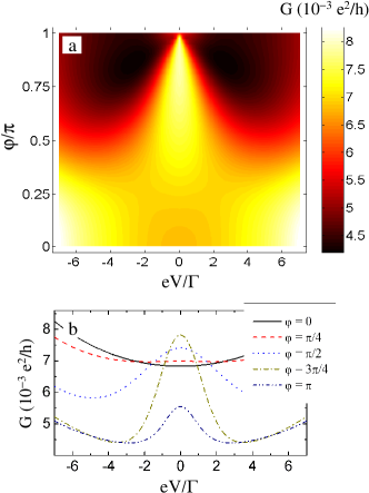
Figure 5: (color online) (a) The differential conductance $G=dI/dV$ as a function of the bias voltage $V$ and the angle $\varphi$ for the asymmetric Anderson model $\varepsilon=-12\Gamma$ and $U=30\Gamma$. The other parameters are the same as in Fig. 2. Part (b) shows the bias dependence of differential conductance for several values of the angle $\varphi$.

The transport characteristics described above for the symmetric Anderson model are significantly modified when the model becomes asymmetric, i.e. when $\varepsilon\neq-U/2$. This can be realized by shifting the dot level position by a gate voltage applied to the dot. Different contributions to the exchange field do not cancel then, and the resulting effective exchange field becomes nonzero. This has a significant impact on transport properties, as we show and discuss below.

First, we note that the leading contribution to the exchange field comes from the first-order diagrams, whereas the current flows due to the second-order tunneling processes. This leads to two different time scales which determine transport characteristics, as will be discussed below in more details. Transport properties are thus a result of the interplay between the first- and second-order processes. We emphasize that although the first-order processes do not contribute directly to the current, they influence transport via modification of the dot spin.

The strength of effective exchange field is determined by deviation of the Anderson model from the symmetric one, described quantitatively by $2\varepsilon+U$ (with $2\varepsilon+U=0$ for the symmetric model). On the other hand, the cotunneling processes contributing to the current are proportional to the bias voltage. Thus, to parameterize relative magnitude of the two processes we define a dimensionless parameter $x=(2\varepsilon+U)/|eV|$.

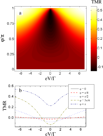
Figure 6: (color online) (a) Tunnel magnetoresistance as a function of the bias voltage $V$ and the angle $\varphi$ for the asymmetric Anderson model. The parameters the same as in Fig. 5. Part (b) shows the TMR as a function of the bias voltage for several values of $\varphi$.

In Fig. 5a we show the differential conductance as a function of angle and bias voltage for an asymmetric Anderson model, $\varepsilon\neq-U/2$, while Fig. 5b displays the bias dependence of $G$ for different values of $\varphi$. As one can see, the low-bias differential conductance becomes enhanced in a certain range of the angle $\varphi$, leading to a nonmonotonic dependence of the conductance $G$ on the angle between the leads’ magnetizations. This nonmonotonic behavior is also visible in TMR. The density plot of TMR is shown in Fig. 6a, whereas the TMR as a function of bias voltage for different values of $\varphi$ is shown in Fig. 6b. There is a range of the angle $\varphi$ between magnetic moments of the leads, where TMR changes sign and becomes negative in the small bias region, i.e. the corresponding conductance is larger than that in the parallel configuration. To discuss and account for the influence of exchange field, we further present one-dimensional figures displaying explicitly the angular dependence of both $G$ and TMR.

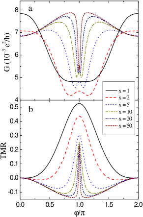
Figure 7: (color online) The differential conductance $G$ (a) and tunnel magnetoresistance (b) as a function of the angle $\varphi$ for several values of $x=(2\varepsilon+U)/|eV|$ and for $\varepsilon=-12\Gamma$. The other parameters are the same as in Fig. 2.

The angular variation of the differential conductance and TMR for an asymmetric Anderson model is shown in Fig. 7 for several values of the parameter $x$, $x=(2\varepsilon+U)/|eV|$. In this figure both $\varepsilon$ and $U$ are kept constant ($\varepsilon=-2U/5$ and $U=30\Gamma$), so the variation of $x$ is only due to the change of the bias voltage. When increasing $x$ (decreasing bias voltage), one increases the relative role of the first-order processes (leading to the spin precession), which considerably modifies the angular dependence of the differential conductance and TMR. As one can see in Fig. 7a, the differential conductance for $x\gg 1$ does not change monotonically with the angle $\varphi$. It increases first with increasing $\varphi$, reaches a local maximum, and then drops to a local minimum for $\varphi$ close to the antiparallel configuration, and again slightly increases when approaching $\varphi=\pi$. Thus, the maximum and minimum differential conductance occur for non-collinear configurations, and not for parallel and antiparallel ones. The local maximum in $G$ at the antiparallel configuration becomes smaller when the effect of exchange field is suppressed ($x$ decreases) and eventually disappears for $x=1$ by transforming into the global minimum of $G$ in the antiparallel configuration. Similarly, the maximum at a non-collinear configuration disappears with decreasing $x$ and changes into a global maximum in the parallel configuration.

The most characteristic features of transport characteristics in the presence of exchange field are the enhanced differential conductance at a non-collinear alignment and its rapid drop when approaching the antiparallel configuration. This is most visible in the curve for $x=50$ in Fig. 7a. In this case the differential conductance increases until the configuration becomes close to the antiparallel one, and then drops rapidly to the value of $G$ in the antiparallel configuration. The key role in this behavior is played by the first-order processes giving rise to the exchange field. These processes lead to the precession of spin in the dot, which facilitates tunneling processes and leads to an increase in the conductance as compared to the parallel configuration. When the configuration becomes close to the antiparallel one, the first-order processes become suppressed and the conductance drops to that for antiparallel alignment. For smaller $x$ the drop in conductance begins at a smaller angle, which follows from the fact that now the relative role of exchange field decreases due to increased cotunneling rates.

The nonmonotonic behavior of the differential conductance with $\varphi$ leads to a nonmonotonic dependence of TMR. This is shown in Fig. 7b for several values of $x$. The effects due to exchange field give rise to a local minimum in TMR at a non-collinear magnetic configuration. Moreover, in this transport regime TMR changes sign and becomes negative. When the magnetic configuration is close to the antiparallel one, TMR starts to increase rapidly reaching maximum for $\varphi=\pi$. The negative TMR and its sudden increase when the configuration tends to the antiparallel one are a consequence of the processes leading to nonmonotonic behavior of the differential conductance, as described above.

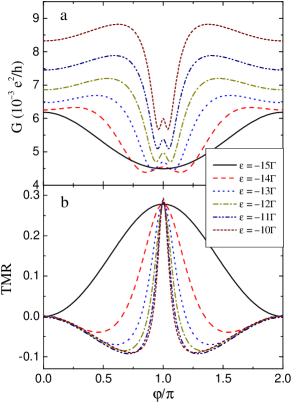
Figure 8: (color online) The differential conductance (a) and tunnel magnetoresistance (b) as a function of angle between the leads’ magnetizations for several values of the level position $\varepsilon$, as indicated in the figure, and for $V=\Gamma$. The other parameters are the same as in Fig. 2.

To understand more intuitively the above presented behavior of the differential conductance and TMR at low bias voltage and close to the antiparallel configuration, one should consider two different time scales. One time scale, $\tau_{\rm prec}$, is established by the virtual first-order processes responsible for the spin precession due to exchange field,

$$\left|\tau^{-1}_{\rm prec}\right|\approx\frac{\Gamma}{2h}p\sin\varphi\ln\left|\frac{\varepsilon}{\varepsilon+U}\right|\,.$$ (28)

The second time scale, $\tau_{\rm cot}$, is associated with second-order processes which drive the current through the system. At low temperature and bias voltage, the cotunneling rate can be expressed as

$$\tau^{-1}_{\rm cot}\approx\frac{\Gamma^{2}}{4h}(1+p)(1-p\cos\varphi)\frac{|eV|U^{2}}{\varepsilon^{2}(\varepsilon+U)^{2}}\,.$$ (29)

The rate $\tau_{\rm cot}$ depends linearly on the applied voltage, whereas $\tau_{\rm prec}$ is rather independent of $V$. As a consequence, at low bias and for non-collinear configuration, the exchange field plays an important role leading to a nonmonotonic dependence of differential conductance on the angle between the leads’ magnetizations. When magnetic configuration is close to the antiparallel one, the spin precession rate is deceased ($\left|\tau^{-1}_{\rm prec}\right|\sim\sin\varphi$) and, at certain angle, the rate of spin precession becomes comparable to the cotunneling rate. This gives rise to a sudden drop (increase) in differential conductance (TMR), as can be seen in Fig. 7a(b). We note that the nonmonotonic dependence of differential conductance and magnetoresistance has also been observed in quantum dots in the strong coupled limit. fransson05

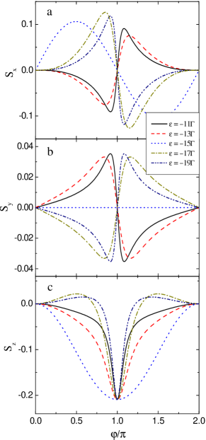
Figure 9: (color online) The $S_{x}$ (a), $S_{y}$ (b), and $S_{z}$ (c) components of the dot spin as a function of angle $\varphi$ for several values of $\varepsilon$ and for $V=\Gamma$. The other parameters are the same as in Fig. 2.

As follows from Eqs. (28) and (29), in the low bias voltage regime the influence of the exchange field is mainly determined by the magnitude of departure from the symmetric Anderson model, $\left|\tau^{-1}_{\rm prec}\right|\sim\ln\left|\varepsilon/(\varepsilon+U)\right|$. The angular variation of the differential conductance and TMR for several values of the level position is shown in Fig. 8. When raising the position of the dot level one goes from the symmetric to asymmetric Anderson model, increasing the effect of exchange field, which is most visible for $\varepsilon=-10\Gamma$. The influence of exchange field is the same as in the case of Fig. 7 discussed above. Figure 8 demonstrates that at a certain non-collinear magnetic configuration, by sweeping the gate voltage one can change the differential conductance and also tune the TMR between the positive and negative values. This can be of some importance for future applications in spintronics.

In the case of symmetric Anderson model the dot spin is located in the plane defined by the magnetizations of the leads, i.e. in the $x-z$ plane. On the other hand, in the case of asymmetric Anderson model, the exchange field gives rise to the spin precession in the dot, leading to a nonzero $S_{y}$ component of the dot spin. The components of the spin in the dot are shown in Fig. 9 for different position of the dot level. If we start from a symmetric Anderson model, then the conductance and TMR are independent of the sign of the dot level shift (shifting the dot level up or down by the same amount leads to equal conductance and TMR). The spin in the dot, however, depends on the sign of the shift. This is due to the fact that changing sign of the shift is associated with a sign change of the exchange field, which is proportional to $\ln|\varepsilon/(\varepsilon+U)|$. As can be seen in Fig. 9, the sign of the exchange field determines the sign of the spin components. It is also worth noting that the two components, $S_{x}$ and $S_{y}$, disappear in both collinear configurations (parallel and antiparallel). In turn the $S_{z}$ component vanishes only in the parallel configuration, while it remains nonzero in the antiparallel configuration due to spin accumulation. weymannPRB06

V Summary and concluding remarks

We have considered the cotunneling transport through a single-level quantum dot coupled to ferromagnetic leads with non-collinearly aligned magnetic moments. Transport properties have been calculated with the aid of the real-time diagrammatic technique which has been adapted to the case of deep Coulomb blockade regime. The advantage of the real-time diagrammatic technique is that it takes into account the exchange field resulting from virtual processes between the dot and ferromagnetic leads in a fully systematic way.

In the case of symmetric Anderson model, we have found a monotonic variation of the differential conductance and TMR with the angle between magnetic moments of the leads. This typical angular dependence is due to the fact that different contributions to the exchange field cancel each other and there is no spin precession of the dot spin – the dot spin remains in the plane defined by the magnetic moments of the leads.

When the system is described by an asymmetric Anderson model, the angular dependence of the differential conductance and TMR becomes more complex. First, the maximum and minimum values of differential conductance occur not for collinear configurations, but when the leads’ magnetizations are non-collinearly aligned. Second, the conductance is enhanced in a broad range of the angle between the magnetic moments of the leads, and drops to the minimum value when the configuration becomes close to the antiparallel one. The conductance drop is particularly pronounced for small bias voltages. This behavior results from the interplay between the first-order processes giving rise to the exchange field and the second-order processes that drive the current. The exchange field also leads to a nonmonotonic angular dependence of TMR. For magnetic configurations where differential conductance is enhanced as compared to that in parallel configuration, the TMR becomes negative.

Appendix A Self-energies in the Coulomb blockade regime

In this appendix we present the analytical formulas for the first- and second-order self-energies involving at the ends the off-diagonal states that are necessary to determine the dot occupations and spin from Eq. (17). Our results are valid in the case of deep Coulomb blockade, $|\varepsilon|,|\varepsilon+U|\gg k_{\rm B}T,\Gamma$. For the first order we find, ${\Sigma_{0\sigma}^{0\bar{\sigma}}}^{(1)}={\Sigma_{{\rm d}\sigma}^{{\rm d}\bar{\sigma}}}^{(1)}=2\pi i\sum_{\alpha}\Gamma_{\alpha}^{\sigma\bar{\sigma}}$, ${\Sigma_{\sigma\sigma}^{\sigma\bar{\sigma}}}^{(1)}={\Sigma_{\sigma\sigma}^{\bar{\sigma}\sigma}}^{(1)}=\sum_{\alpha}\left(B_{1\alpha}^{\sigma\bar{\sigma}}-C_{1\alpha}^{\sigma\bar{\sigma}}\right)$, and ${\Sigma^{\sigma\sigma}_{\bar{\sigma}\bar{\sigma}}}^{(1)}=\sum_{\alpha}\left(B_{1\alpha}^{\sigma\sigma}-B_{1\alpha}^{\bar{\sigma}\bar{\sigma}}+C_{1\alpha}^{\bar{\sigma}\bar{\sigma}}-C_{1\alpha}^{\sigma\sigma}\right)$, where $\alpha={\rm L,R}$.

The imaginary parts of the second-order self-energies involving off-diagonal states are given by

$${\rm Im}{\Sigma_{\sigma\sigma}^{\sigma\bar{\sigma}}}^{(2)}=\pi\sum_{\alpha,\beta}\sum_{\sigma^{\prime}}\bigg{[}2\Gamma_{\alpha}^{\sigma\bar{\sigma}}\left(B_{2\beta}^{\sigma\sigma}+C_{2\beta}^{\bar{\sigma}\bar{\sigma}}\right)$$ (30)

$$+ 2B_{2\alpha\beta}^{\sigma\sigma,\sigma\bar{\sigma}}-B_{2\alpha\beta}^{\sigma\bar{\sigma},\sigma^{\prime}\sigma^{\prime}}+2C_{2\alpha\beta}^{\sigma\bar{\sigma},\bar{\sigma}\bar{\sigma}}-C_{2\alpha\beta}^{\sigma^{\prime}\sigma^{\prime},\sigma\bar{\sigma}}$$

$$+ \frac{1}{U}\left(A_{1\alpha\beta}^{\bar{\sigma}\bar{\sigma},\sigma\bar{\sigma}}-A_{1\alpha\beta}^{\sigma\bar{\sigma},\sigma\sigma}+3A_{1\alpha\beta}^{\sigma\sigma,\sigma\bar{\sigma}}-3A_{1\alpha\beta}^{\sigma\bar{\sigma},\bar{\sigma}\bar{\sigma}}\right)\bigg{]}\,,$$

$${\rm Im}{\Sigma_{\sigma\sigma}^{\bar{\sigma}\sigma}}^{(2)}=\pi\sum_{\alpha,\beta}\bigg{[}2\Gamma_{\alpha}^{\sigma\sigma}B_{2\beta}^{\sigma\bar{\sigma}}+2\Gamma_{\alpha}^{\bar{\sigma}\bar{\sigma}}C_{2\beta}^{\sigma\bar{\sigma}}$$ (31)

$$+ B_{2\alpha\beta}^{\sigma\bar{\sigma},\sigma\sigma}-B_{2\alpha\beta}^{\sigma\bar{\sigma},\bar{\sigma}\bar{\sigma}}+C_{2\alpha\beta}^{\sigma\sigma,\sigma\bar{\sigma}}-C_{2\alpha\beta}^{\bar{\sigma}\bar{\sigma},\sigma\bar{\sigma}}$$

$$+ \frac{1}{U}\left(A_{1\alpha\beta}^{\sigma\sigma,\sigma\bar{\sigma}}-A_{1\alpha\beta}^{\bar{\sigma}\bar{\sigma},\sigma\bar{\sigma}}+A_{1\alpha\beta}^{\sigma\bar{\sigma},\sigma\sigma}-A_{1\alpha\beta}^{\sigma\bar{\sigma},\bar{\sigma}\bar{\sigma}}\right)\bigg{]}\,,$$

$${\rm Im}{\Sigma_{\bar{\sigma}\sigma}^{\sigma\bar{\sigma}}}^{(2)}=2\pi\sum_{\alpha,\beta}\bigg{[}\Gamma_{\alpha}^{\sigma\bar{\sigma}}B_{2\beta}^{\sigma\bar{\sigma}}-\Gamma_{\alpha}^{\sigma\bar{\sigma}}C_{2\beta}^{\sigma\bar{\sigma}}$$ (32)

$$+ B_{2\alpha\beta}^{\sigma\bar{\sigma},\sigma\bar{\sigma}}+C_{2\alpha\beta}^{\sigma\bar{\sigma},\sigma\bar{\sigma}}+\frac{2}{U}A_{1\alpha\beta}^{\sigma\bar{\sigma},\sigma\bar{\sigma}}\bigg{]}\,,$$

$${\rm Im}{\Sigma_{\bar{\sigma}\bar{\sigma}}^{\sigma\sigma}}^{(2)}=\pi\sum_{\alpha,\beta}\sum_{\sigma^{\prime},\sigma^{\prime\prime}}\bigg{[}2\Gamma_{\alpha}^{\sigma\bar{\sigma}}\left(B_{2\beta}^{\sigma\bar{\sigma}}-C_{2\beta}^{\sigma\bar{\sigma}}\right)$$ (33)

$$+ 2B_{2\alpha\beta}^{\sigma\bar{\sigma},\sigma\bar{\sigma}}+2C_{2\alpha\beta}^{\sigma\bar{\sigma},\sigma\bar{\sigma}}-B_{2\alpha\beta}^{\sigma^{\prime}\sigma^{\prime},\sigma^{\prime\prime}\sigma^{\prime\prime}}-C_{2\alpha\beta}^{\sigma^{\prime}\sigma^{\prime},\sigma^{\prime\prime}\sigma^{\prime\prime}}$$

$$+ \frac{2}{U}\left(2A_{1\alpha\beta}^{\sigma\bar{\sigma},\sigma\bar{\sigma}}-A_{1\alpha\beta}^{\sigma^{\prime}\sigma^{\prime},\sigma^{\prime\prime}\sigma^{\prime\prime}}\right)\bigg{]}\,,$$

$${\rm Im}{\Sigma_{\bar{\sigma}0}^{\sigma 0}}^{(2)}=2\pi\sum_{\alpha,\beta}\left(\Gamma_{\alpha}^{\sigma\sigma}+\Gamma_{\alpha}^{\bar{\sigma}\bar{\sigma}}\right)B_{2\beta}^{\sigma\bar{\sigma}}\,,$$ (34)

where $\alpha,\beta={\rm L,R}$ and $\sigma^{\prime},\sigma^{\prime\prime}=\sigma,\bar{\sigma}$. The corresponding parameters are defined as

$$B_{n\alpha}^{\sigma\sigma^{\prime}}=\Gamma_{\alpha}^{\sigma\sigma^{\prime}}X_{n}(\varepsilon-\mu_{\alpha})\,,$$ (35)

$$B_{n\alpha\beta}^{\sigma\sigma^{\prime}\sigma^{\prime\prime}\sigma^{\prime\prime\prime}} = \Gamma_{\alpha}^{\sigma\sigma^{\prime}}\Gamma_{\beta}^{\sigma^{\prime\prime}\sigma^{\prime\prime\prime}}f_{\rm B}(\mu_{\alpha}-\mu_{\beta})$$ (36)

$$\times \left[X_{n}(\varepsilon-\mu_{\alpha})-X_{n}(\varepsilon-\mu_{\beta})\right]\,,$$

with

$$X_{n+1}(x)=\frac{d^{(n)}}{dx^{(n)}}{\rm Re}\left[\Psi\left(\frac{1}{2}+i\frac{x}{2\pi k_{\rm B}T}\right)-\ln\left(\frac{W}{2\pi k_{\rm B}T}\right)\right]\,,$$ (37)

where $W$ is the cutoff parameter and $f_{\rm B}$ denotes the Bose function. The parameters $C_{n\alpha}^{\sigma\sigma^{\prime}}$ and $C_{n\alpha\beta}^{\sigma\sigma^{\prime}\sigma^{\prime\prime}\sigma^{\prime\prime\prime}}$ are given by Eqs. (35) and (36), respectively, with $\varepsilon$ replaced by $\varepsilon+U$, while $A_{n\alpha\beta}^{\sigma\sigma^{\prime}\sigma^{\prime\prime}\sigma^{\prime\prime\prime}}=B_{n\alpha\beta}^{\sigma\sigma^{\prime}\sigma^{\prime\prime}\sigma^{\prime\prime\prime}}-C_{n\alpha\beta}^{\sigma\sigma^{\prime}\sigma^{\prime\prime}\sigma^{\prime\prime\prime}}$. The other self-energies can be found using the rules and relations given in section III.1.

Appendix B Green’s functions in the Coulomb blockade regime

In the following we present the explicit formulas for the Green’s functions needed to calculate the current in the case of the Coulomb blockade regime. The Green’s functions $G_{\sigma\sigma^{\prime}}^{\lessgtr(1,0)}$ are given by $G_{\sigma\sigma}^{>(1,0)}=-2\pi i{P_{0}^{0}}^{(1)}\delta(\omega-\varepsilon)$, $G_{\sigma\sigma}^{<(1,0)}=2\pi i{P_{\rm d}^{\rm d}}^{(1)}\delta(\omega-\varepsilon-U)$, while $G_{\sigma\bar{\sigma}}^{\lessgtr(1,0)}=0$. On the other hand, for $G_{\sigma\sigma^{\prime}}^{\lessgtr(0,1)}$ we find

$$G_{\sigma\sigma}^{>(0,1)} = -2\pi i\sum_{\sigma^{\prime}}\left\{{P_{\sigma^{\prime}}^{\sigma^{\prime}}}^{(0)}\left[b_{2\alpha}^{-\sigma^{\prime}\sigma^{\prime}}+B_{2\alpha}^{\sigma^{\prime}\sigma^{\prime}}\delta(\omega-\varepsilon)\right]\right.$$ (38)

$$+{P_{\bar{\sigma}}^{\bar{\sigma}}}^{(0)}\left[c_{2\alpha}^{-\sigma^{\prime}\sigma^{\prime}}+\frac{2}{U}\left(b_{1\alpha}^{-\bar{\sigma}\bar{\sigma}}-c_{1\alpha}^{-\bar{\sigma}\bar{\sigma}}\right)\right]$$

$$+2S_{x}^{(0)}\left[b_{2\alpha}^{-\sigma\bar{\sigma}}+B_{2\alpha}^{\sigma\bar{\sigma}}\delta(\omega-\varepsilon)\right.$$

$$\left.\left.+\frac{1}{U}\left(b_{1\alpha}^{-\sigma\bar{\sigma}}-c_{1\alpha}^{-\sigma\bar{\sigma}}\right)\right]\right\}\,,$$

$$G_{\sigma\bar{\sigma}}^{>(0,1)} = 2\pi i\left\{S_{x}^{(0)}\sum_{\sigma^{\prime}}\left[c_{2\alpha}^{-\sigma^{\prime}\sigma^{\prime}}+\frac{1}{U}\left(b_{1\alpha}^{-\sigma^{\prime}\sigma^{\prime}}-c_{1\alpha}^{-\sigma^{\prime}\sigma^{\prime}}\right)\right]\right.$$ (39)

$$\left.+\frac{1}{U}\left[{P_{\sigma}^{\sigma}}^{(0)}+{P_{\bar{\sigma}}^{\bar{\sigma}}}^{(0)}\right]\left(b_{1\alpha}^{-\sigma\bar{\sigma}}-c_{1\alpha}^{-\sigma\bar{\sigma}}\right)\right\}\,,$$

$$G_{\sigma\sigma}^{<(0,1)} = 2\pi i\sum_{\sigma^{\prime}}\left\{{P_{\bar{\sigma}^{\prime}}^{\bar{\sigma}^{\prime}}}^{(0)}\left[c_{2\alpha}^{+\sigma^{\prime}\sigma^{\prime}}-C_{2\alpha}^{\sigma^{\prime}\sigma^{\prime}}\delta(\omega-\varepsilon-U)\right]\right.$$ (40)

$$+{P_{\sigma}^{\sigma}}^{(0)}\left[b_{2\alpha}^{+\sigma^{\prime}\sigma^{\prime}}+\frac{2}{U}\left(b_{1\alpha}^{+\bar{\sigma}\bar{\sigma}}-c_{1\alpha}^{+\bar{\sigma}\bar{\sigma}}\right)\right]$$

$$-2S_{x}^{(0)}\left[c_{2\alpha}^{+\sigma\bar{\sigma}}-C_{2\alpha}^{\sigma\bar{\sigma}}\delta(\omega-\varepsilon-U)\right.$$

$$\left.\left.+\frac{1}{U}\left(b_{1\alpha}^{+\sigma\bar{\sigma}}-c_{1\alpha}^{+\sigma\bar{\sigma}}\right)\right]\right\}\,,$$

$$G_{\sigma\bar{\sigma}}^{<(0,1)} = 2\pi i\left\{S_{x}^{(0)}\sum_{\sigma^{\prime}}\left[b_{2\alpha}^{+\sigma^{\prime}\sigma^{\prime}}+\frac{1}{U}\left(b_{1\alpha}^{+\sigma^{\prime}\sigma^{\prime}}-c_{1\alpha}^{+\sigma^{\prime}\sigma^{\prime}}\right)\right]\right.$$ (41)

$$\left.-\frac{1}{U}\left[{P_{\sigma}^{\sigma}}^{(0)}+{P_{\bar{\sigma}}^{\bar{\sigma}}}^{(0)}\right]\left(b_{1\alpha}^{+\sigma\bar{\sigma}}-c_{1\alpha}^{+\sigma\bar{\sigma}}\right)\right\}\,,$$

with

$$b_{n\alpha}^{\pm\sigma\sigma^{\prime}}=\frac{\gamma_{\alpha}^{\pm\sigma\sigma^{\prime}}(\omega)}{(\omega-\varepsilon)^{n}}\,,$$ (42)

and $c_{n\alpha}^{\pm\sigma\sigma^{\prime}}$ is given by Eq. (42) with $\varepsilon\leftrightarrow\varepsilon+U$, while the other parameters are defined in Appendix A. In the above formulas we have cancelled all the terms whose contribution to the current is exponentially suppressed, i.e., the terms multiplied with $\delta(\omega-\varepsilon)$ and $\delta(\omega-\varepsilon-U)$ in $G_{\sigma\sigma^{\prime}}^{<(0,1)}$ and $G_{\sigma\sigma^{\prime}}^{>(0,1)}$, respectively, as well as the terms multiplied with $\delta^{\prime}(\omega-\varepsilon)$ and $\delta^{\prime}(\omega-\varepsilon-U)$, where $\delta$ is the Dirac function and $\delta^{\prime}$ its derivative.

References

- (1) S. A. Wolf, D. D. Awschalom, R. A. Buhrman, J. M. Daughton, S. von Molnar, M. L. Roukes, A. Y. Chtchelka, and D. M. Treger, Science 294, 1488 (2001).
- (2) Semiconductor Spintronics and Quantum Computation, ed. by D. D. Awschalom, D. Loss, and N. Samarth (Springer, Berlin 2002).
- (3) S. Maekawa and T. Shinjo, Spin Dependent Transport in Magnetic Nanostructures (Taylor & Francis 2002).
- (4) I. Zutic, J. Fabian, S. Das Sarma, Rev. Mod. Phys. 76, 323 (2004).
- (5) N. Sergueev, Qing-feng Sun, Hong Guo, B. G. Wang, and Jian Wang, Phys. Rev. B 65, 165303 (2002).
- (6) R. López and D. Sánchez, Phys. Rev. Lett. 90, 116602 (2003).
- (7) J. Martinek, Y. Utsumi, H. Imamura, J. Barnaś, S. Maekawa, J. König, and G. Schön, Phys. Rev. Lett. 91, 127203 (2003).
- (8) J. Fransson, Phys. Rev. B 72, 045415 (2005); Europhys. Lett. 70, 796 (2005).
- (9) Y. Utsumi, J. Martinek, G. Schön, H. Imamura, and S. Maekawa, Phys. Rev. B 71, 245116 (2005).
- (10) R. Świrkowicz, M. Wilczyński, M. Wawrzyniak, and J. Barnaś, Phys. Rev. B 73, 193312 (2006).
- (11) D. Matsubayashi, M. Eto, cond-mat/0607548 (unpublished); P. Simon, P. S. Cornaglia, D. Feinberg, C. A. Balseiro, cond-mat/0607794 (unpublished).
- (12) Single Charge Tunneling: Coulomb Blockade Phenomena in Nanostructures, NATO ASI Series B: Physics 294, ed. by H. Grabert, M. H. Devoret (Plenum Press, New York 1992).
- (13) L. P. Kouwenhoven, C. M. Marcus, P. L. McEuen, S. Tarucha, R. M. Westervelt, and N. S. Wingreen, in Proceedings of the NATO Advanced Study Institute on Mesoscopic Electron Transport, ed. by L. L. Sohn, L. P. Kouwenhoven, and G. Schön (Kluwer Series E345, 1997).
- (14) D. V. Averin and A. A. Odintsov, Phys. Lett. A 140, 251 (1989).
- (15) D. V. Averin and Yu. V. Nazarov, Phys. Rev. Lett. 65, 2446 (1990).
- (16) K. Kang and B. I. Min, Phys. Rev. B 55, 15412 (1997).
- (17) B. R. Bułka, Phys. Rev. B 62, 1186 (2000).
- (18) W. Rudziński and J. Barnaś, Phys. Rev. B 64, 085318 (2001).
- (19) J. König and J. Martinek, Phys. Rev. Lett. 90, 166602 (2003); M. Braun, J. König, J. Martinek, Phys. Rev. B 70, 195345 (2004).
- (20) W. Rudziński, J. Barnaś, R. Świrkowicz, and M. Wilczyński, Phys. Rev. B 71, 205307 (2005); J. Mag. Mag. Mat. 294, 1 (2005).
- (21) W. Wetzels and G. E. W. Bauer, M. Grifoni, Phys. Rev. B 72, 020407(R) (2005).
- (22) M. Braun, J. König, J. Martinek, Phys. Rev. B 74, 075328 (2006).
- (23) I. Weymann, J. Barnaś, J. König, J. Martinek, and G. Schön, Phys. Rev. B 72, 113301 (2005).
- (24) I. Weymann, J. König, J. Martinek, J. Barnaś, and G. Schön, Phys. Rev. B 72, 115334 (2005).
- (25) I. Weymann and J. Barnaś, Phys. Rev. B 73, 205309 (2006).
- (26) J. N. Pedersen, J. Q. Thomassen, and K. Flensberg, Phys. Rev. B 72, 045341 (2005).
- (27) S. Braig and P. W. Brouwer, Phys. Rev. B 71, 195324 (2005).
- (28) I. Weymann and J. Barnaś, Eur. Phys. J. B 46, 289 (2005).
- (29) I. Weymann, cond-mat/0610768 (unpublished).
- (30) L. Y. Zhang, C. Y. Wang, Y. G. Wei, X. Y. Liu, and D. Davidović, Phys. Rev. B 72, 155445 (2005).
- (31) K. Tsukagoshi, B. W. Alphenaar, and H. Ago, Nature 401, 572 (1999).
- (32) B. Zhao, I. Mönch, H. Vinzelberg, T. Mühl, and C. M. Schneider, Appl. Phys. Lett. 80, 3144 (2002); J. Appl. Phys. 91, 7026 (2002).
- (33) A. Jensen, J. R. Hauptmann, J. Nygard, and P. E. Lindelof, Phys. Rev. B 72, 035419 (2005).
- (34) S. Sahoo, T. Kontos, J. Furer, C. Hoffmann, M. Gräber, A. Cottet, and C. Schönenberger, Nature Physics 1, 102 (2005).
- (35) A. N. Pasupathy, R. C. Bialczak, J. Martinek, J. E. Grose, L. A. K. Donev, P. L. McEuen, and D. C. Ralph, Science 306, 86 (2004).
- (36) A. Bernand-Mantel, P. Seneor, N. Lidgi, M. Munoz, V. Cros, S. Fusil, K. Bouzehouane, C. Deranlot, A. Vaures, F. Petroff, and A. Fert, Appl. Phys. Lett. 89, 062502 (2006).
- (37) K. Hamaya, S. Masubuchi, M. Kawamura, and T. Machida, M. Jung, K. Shibata, and K. Hirakawa, T. Taniyama, S. Ishida and Y. Arakawa, cond-mat/0611269 (unpublished).
- (38) A. Kogan, S. Amasha, D. Goldhaber-Gordon, G. Granger, M.A. Kastner, and H. Shtrikman, Phys. Rev. Lett. 93, 166602 (2004).
- (39) H. Schoeller and G. Schön, Phys. Rev. B 50, 18436 (1994); J. König, J. Schmid, H. Schoeller, and G. Schön, Phys. Rev. B 54, 16820 (1996).
- (40) J. König, Quantum Fluctuations in the Single-Electron Transistor, (Shaker, Aachen, 1999).
- (41) Hai-Feng Mu, Gang Su, Qing-Rong Zheng, Phys. Rev. B 73, 054414 (2006).
- (42) Y. Meir and N. S. Wingreen, Phys. Rev. Lett. 68, 2512 (1992).