Phase transitions of barotropic flow coupled to a massive rotating sphere - derivation of a fixed point equation by the Bragg method

Abstract

The kinetic energy of barotropic flow coupled to an infnitely massive rotating sphere by an unresolved complex torque mechanism is approximated by a discrete spin-lattice model of fluid vorticity on a rotating sphere, analogous to a one-step renormalized Ising model on a sphere with global interactions. The constrained energy functional is a function of spin-spin coupling and spin coupling with the rotation of the sphere. A mean field approximation similar to the Curie-Weiss theory, modeled after that used by Bragg and Williams to treat a two dimensional Ising model of ferromagnetism, is used to find the barotropic vorticity states at thermal equilibrium for given temperature and rotational frequency of the sphere. A fixed point equation for the most probable barotropic flow state is one of the main results.

This provides a crude model of super and sub-rotating planetary atmospheres in which the barotropic flow can be considered to be the vertically averaged rotating stratified atmosphere and where a key order parameter is the changeable amount of angular momentum in the barotropic fluid. Using the crudest two domains partition of the resulting fixed point equation, we find that in positive temperatures associated with low energy flows, for fixed planetary spin larger than $\Omega_{c}>0$ there is a continuous transition from a disordered state in higher temperatures to a counter-rotating solid-body flow state in lower positive temperatures. The most probable state is a weakly counter-rotating mixed state for all positive temperatures when planetary spin is smaller than $\Omega_{c}.$

For sufficiently large spins $\Omega>2\Omega_{c}$, there is a single smooth change from slightly pro-rotating mixed states to a strongly pro-rotating ordered state as the negative value of $T$ increases (or decreases in absolute value). But for smaller spins $\Omega<2\Omega_{c}$ there is a transition from a predominantly mixed state (for $T\ll-1)$ to a pro-rotating state at $\beta^{-}(\Omega)<0$ plus a second $\beta_{c}^{\Omega},$ for which the fixed point equation has three fixed points when $\beta<\beta_{c}^{\Omega}$ instead of just the pro-rotating one when $\beta_{c}^{\Omega}<\beta.$ An argument based on comparing free energy show that the pro-rotating state is preferred when there are three fixed points because it has the highest free energy - at negative temperatures the thermodynamically stable state is the one with the maximum free energy.

In the non-rotating case ($\Omega=0)$ the most probable state changes from a mixed state for all positive and large absolute-valued negative temperatures to an ordered state of solid-body flow at small absolute-valued negative temperatures through a standard symmetry-breaking second order phase transition. The predictions of this model for the non-rotating problem and the rotating problem agrees with the predictions of the simple mean field model and the spherical model.

This model differs from previous mean field theories for quasi-2D turbulence in not fixing angular momentum nor relative enstrophy - a property which increases its applicability to coupled fluid-sphere systems and by extension to 2d turbulent flows in complex domains such as no-slip square boundaries where only the total circulation are fixed - as opposed to classical statistical equilibrium models such as the vortex gas model and Miller-Robert theories that fix all the vorticity moments. Furthermore, this Bragg mean field theory is well-defined for all positive and negative temperatures unlike the classical energy-enstrophy theories.

1 Introduction

Previous statistical equilibrium studies of inviscid flows on a rotating sphere with trivial topography focussed on the classical energy-enstrophy formulation [17] of PDE models such as in [16] did not find any phase transitions [18] to super-rotating solid-body flows. The main reason is that these Hamiltonian PDE models which conserve the angular momentum of the fluid, are not suited to the study of a phenomena like the super-rotation of the Venusian middle atmosphere that depends on transfer of angular momentum between the atmosphere and the solid planet.

We therefore consider instead a single layer of barotropic fluid of fixed height coupled by a complex torque mechanism to a massive rotating sphere as a simplified model of planetary atmosphere. The approach in this paper is to consider different possible thermodynamic properties of the steady states of coupled planetary atmospheres as mean field statistical equilibria - through a natural relation of fluid vorticity systems to electromagnetic models - with the aim of showing explicitly that sub-rotating and super-rotating flow states can arise spontaneously from random initial states.

A simple mean field method on a related model [19], (where spins are allowed to take on a continuous range of values), has successfully found phase transitions for barotropic flows coupled to a rotating sphere. There as here, angular momentum of the fluid is allowed to change; and the expected values of total circulation and relative enstrophy are fixed in this simple mean field theory. This leads to the exciting result that sub-rotational and super-rotational macrostates are preferred in certain thermodynamic regimes. The Bragg mean field theory presented in this paper corroborates some of these previous results but has the important new property that relative enstrophy is constrained only by an inequality while total circulation is held fixed at zero. Further discussion of these important points will follow in the next section.

Our results are also in agreement with Monte Carlo simulations on the logarithmic spherical model in the non-rotating case [15] and the rotating sphere [1], [4]. The phrase spherical model refers to the fact that under a discrete approximation, the microcanonical constraint on the relative enstrophy becomes a spherical constraint first introduced by Kac [18]. We shift gears here from the spherical model used by Lim - for which closed form solutions of the partition function required considerable analytical effort [12], [5] - to a simplified discrete spin model which enables us to use the Bragg method to approximate the free energy, which in turn allows us to find an interesting analytical solution to the coarse grained stream function for the resulting mean field theory. While the overall qualitative agreement between this Bragg model, Lim’s exact solution of the spherical model and the simple mean field model mentioned above is good, there are subtle differences in the detailed predictions of these models. They are however all within the scope of applications to super and sub-rotations in planetary atmospheres such as on Venus, chiefly because current observations are not refined enough to distinguish between them. It will be necessary to perform detailed direct numerical simulations of coupled geophysical flows in order to gather enough data for a future comparative study which can choose between these three models. Nonetheless, we will discuss in the next section how purely theoretical considerations of the complex boundary conditions that exist in the coupled barotropic fluid -sphere system and in a class of quasi-2d turbulent flows in complex domains allow us to choose the current set of spin-lattice / Eulerian vorticity models with minimal constraints over the vortex gas / Lagrangian models [13], [8] and Miller-Robert theories [9], [10].

Our discrete vorticity model is a set $\mathbf{{X}=}$ $\left\{\vec{x_{i}}\right\}$ of $2N$ random sites on the sphere with uniform distribution, each with a spin $s_{i}\in\left\{+1,-1\right\}$, and interaction energy with every other site as a function of distance. Each spin also interacts with the planetary spin which is analogous to an external magnetic field in the Ising model - the sum of this interaction is proportional to the varying net angular momentum of the fluid relative to a frame that is rotating at the angular velocity of the solid sphere. Contribution to the kinetic energy from planetary spin varies zonally, however, and this makes the external field inhomogeneous and difficult to deal with analytically. Bragg and Williams [2] used a one step renormalization to investigate properties of order-disorder in the Ising Model of a ferromagnet. As the discretized model for barotropic flows coupled to a rotating sphere is similar to the Ising Model of a ferromagnet in an inhomogeneous field, we use the Bragg-Williams renormalization technique to infer the order-disorder properties of the fluid.

It is a well established fact [13] that systems of constrained vortices have both positive and negative temperatures, and the present model is no exception. In this setup, using the simplest two domains partition of the surface of the sphere, we find a positive temperature continuous phase transition to the sub-rotating ordered state for decreasing temperatures if the planetary spin is large enough. There is no evidence of a phase transition for a non-rotating sphere in positive temperature. We also find transitions to a super-rotating ordered state when the negative temperature has small absolute values - that is for very high energy.

2 Statistical mechanics of macroscopic flows

Here we summarize some of the pertinent points concerning the application of a statistical equilibrium approach to macroscopic flows. The largely 2-d flows we are concerned with in this paper are in actuality non-equilibrium phenomena even in the case of nearly inviscid flows - an assumption that is mainly correct for the interior of geophysical flows. The main reason that equilibrium statistical mechanics is applicable here - the existence of two separate time scales in the microdynamics of 2D vorticity - is best formulated as the well-known physical principle of selective decay which states that the slow time scale given by the overall decay rates of enstrophy and kinetic energy in damped unforced flows is sufficiently distinct from the fast time scale corresponding to the inverse cascade relaxation of kinetic energy from small to large spatial scales so that several relaxation periods fits in a unit of slow time. That means that the total kinetic energy (and enstrophy) may be considered fixed in the time it takes for the eddies to reach statistical equilibrium. Furthermore, the principle of selective decay states that the asymptotic properties of the damped 2d flow is characterized by a minimal enstrophy to energy ratio which is dependent on the geometry of the flow domain. One of the key properties of enstrophy known as the square-norm of the vorticity field then implies that these minimum enstrophy states are associated with large scale ordered structures such as domain scale vortices. In the case of the specific problem in this paper, these coherent structures are super- and sub-rotating solid-body flow states.

Aside from the above general points on the applicability of equilibrium statistical mechanics to 2D macroscopic flows, the specific properties of a given flow problem [6] will decide which one of the many statistical equilibrium models [13], [8], [17], [9], [10] is suitable. The coupled nature of the flow problem in this paper where a complex torque mechanism transfers angular momentum and energy between the fluid and rotating solid sphere, clearly eliminates all Lagrangian or vortex gas models [13], [8] on the surface $S^{2}$ because they conserve angular momentum - a result that follows directly from Noether’s theorem. Moreover, since none of the vorticity moments are conserved in the coupled flows except for total circulation which is fixed at zero by Stokes theorem, independently (or in spite) of the coupling between fluid and solid sphere, the Miller-Robert class of models [9], [10] cannot be used here because they are designed to fix all the vorticity moments. It is therefore not surprising that a significant discrepancy was found between statistical equilibrium predictions based on a vortex gas theory and experimental (and direct numerical simulations) of decaying quasi-2D flows in a rectangular box with no-slip boundary conditions [6].

What remains are the classical Kraichnan models - also known as absolute equilibrium models - and variants such as those used in [16]. The problem with these are two-fold - (i) they model a 2d fluid flow that is uncoupled to any boundary or has periodic boundaries and hence angular momentum is held fixed - clearly unsuitable for our aims here, and (ii) they are equivalent to the ubiquitous Gaussian model and can be easily shown to not have well-defined partition functions at low temperatures. One solution taken up in [12], [5] is to impose instead of a canonical enstrophy constraint, a microcanonical one which leads to a version of Kac’s spherical model. Combined with zero total circulation and allowing angular momentum to fluctuate - that is coupling the barotropic fluid to an infinitely massive rotating solid sphere- this approach yielded exact partition functions and closed form expressions for phase transitions to self-organized (or condensed) super- and sub-rotating flows. As expected, these analytic results agree perfectly with Monte-Carlo simulations of the spherical model in [15], [1], [4]. An argument similar in style to the above discussion of the Principle of Selective Decay was needed to justify the choice of a microcanonical (and hence spherical) constraint on relative enstrophy in this class of coupled flows while the zero total circulation constraint needs none since it is implied by topological arguments - Stokes theorem on the sphere. The spherical model unlike the Bragg model in this paper is not based on a mean field assumption. This can be a significant advantage only in modelling more complex geophysical flows where large deviations techniques cannot be used to establish the asymptotic exactness of the mean field.

One of the aims of this paper is therefore to relax the enstrophy constraint - that is, we impose neither a canonical enstrophy constraint like in [17] nor a microcanonical enstrophy constraint like in [12], [5], [15], [1], [4] - and still derive a physically sound mean field theory for a comparatively simple geophysical problem. We will show that the relative enstrophy in the Bragg mean field theory is constrained instead by an upper bound.

Another aim in this paper is to show that the Bragg method can be extended to the situation as in this coupled flow where the kinetic energy is just a functional and not a Hamiltonian of the barotropic flow. This is a subtle but relevant point because the original Bragg method formulated for the Ising model of ferromagnetism worked with a Hamiltonian. The first author reported in [5] and [1], [4] that the kinetic energy of the fluid component of the coupled fluid - rotating sphere system cannot be a Hamiltonian for the evolution of the vorticity field because otherwise its $SO(2)$ symmetry - a property that is easily shown - implies the conservation of angular momentum of the fluid component.

3 Coupled Barotropic Fluid - Rotating Sphere model

We are interested in the physical possibility of planetary atmosphere at thermal equilibrium with the rotating solid planet - the massive sphere is treated as an infinite reservoir for both kinetic energy and angular momentum of the barotropic (vertically averaged) component of the fluid. Thus we consider the atmosphere as a single layer of incompressible inviscid fluid interacting through an unresolved complex torque mechanism with the solid sphere. This is equivalent to formulating a Gibbs canonical ensemble in the energy of the fluid with an implicit canonical constraint on the angular momentum of the fluid. More realistic models include effects of forcing and damping, from solar and ’ground’ interaction as well as internal friction.

As our interest is in global weather patterns, we will consider the problem on the spherical geometry, with non-negative planetary angular velocity $\Omega\geq 0$, and relative stream function $\psi$ - a characteristic of 2-d flows; $q$ describes the total vorticity on the sphere,

$$q=\omega+2\Omega\cos{(\theta)}$$

where the first term $\omega$ is the vorticity relative to the rotating frame in which the sphere is at rest, and the second gives planetary vorticity due to the angular velocity of the sphere in terms of the rotational frequency $\Omega$ and the co-latitude $\theta$. We note the fact that a distinguished rotating frame with fixed rotation rate $\Omega\geq 0$ can be taken to be that in which the sphere is at rest only if the assumption of infinite mass is made. For otherwise, the sphere will rotate at variable rate in response to the instantaneous amount of angular momentum in the fluid component of the coupled system, to conserve the combined angular momentum.

Recall that the vorticity is given by the Laplacian of the stream function,

$$\omega=\Delta\psi$$

In order to study the problem in a more tractable framework, we restate the problem in terms of local vorticity or lattice spins, following Lim [3]. The relative zonal and meridional flow is given by the gradient of the stream function and will be denoted as $u_{r}$ and $v_{r}$ respectively. In addition the flow due to rotation also contributes to the kinetic energy, it is entirely zonal and will be denoted as $u_{p}$. The kinetic energy in the inertial frame will be the key objective functional in our work,

$$H^{\prime}[q] = \frac{1}{2}\int_{S^{2}}dx\left[(u_{r}+u_{p})^{2}+v_{r}^{2}\right]$$ (1)

$$= \frac{1}{2}\int_{S^{2}}dx\left[u_{r}^{2}+v_{r}^{2}+2u_{r}u_{p}+u_{p}^{2}\right]$$ (2)

$$= -\frac{1}{2}\int_{S^{2}}dxq\psi+\frac{1}{2}\int_{S^{2}}dxu_{p}^{2}.$$ (3)

The constant term $\frac{1}{2}\left\|u_{p}\right\|_{2}^{2}$ will be discarded below - we thus work with the pseudo-kinetic energy.

Note that Stokes theorem implies that circulation on the sphere with respect to the rotating frame is zero,

$$\int_{S^{2}}\omega=0$$ (4)

4 The Discrete Model

In the above discussion the relative vorticity is a function on $S^{2}$ given by the Laplacian of the stream function. [11], [19], [3], [4] utilize a transformation to restate the coupled fluid-sphere model in terms of a relative vorticity distribution on the sphere which is then approximated over a discrete lattice. Proceeding from this transformation we consider a model defined by a uniform distribution of nodes $\{x_{i}\}$ on the sphere; edges spanning a pair of sites $x_{i},x_{j}$ are assigned interaction energy $J_{(i,j)}$. The kinetic energy of the fluid component is then given by pairwise coupling of local vorticity and coupling of local vorticity to the planetary spin. Without loss of generality - for a single step renormalization based on block spins later relates this Ising model to a more physical model with real valued spins - we consider only local vorticity with spin of $+1$ or $-1$. As these spins are intended to model fluid flow, Stokes’ theorem requires for $2N$ vortices of equal magnitude on the sphere that $N$ vortices be of $+1$ spin and $N$ vortices be of $-1$ spin. Under this restriction we consider the state space with the objective of finding the statistically preferred states.

Formally, the state space consists of functions of the form

$$\omega(x)=\sum_{i}H_{i}(x)s_{i}$$

where

$$H_{i}=\frac{{4\pi}}{N}\delta(x_{i}-x).$$

The vorticity $s_{i}$ is assigned values $\pm 1$ which models the direction of the spin at a node. Thus we have the following simple form for the kinetic energy of the system, as a discrete approximation to the pseudo-kinetic energy,

$$H_{N}=-\sum_{(i,j)}\,^{\prime}J_{(i,j)}s_{i}s_{j}-\Omega\sum_{i}F_{i}s_{i}$$ (5)

where $\sum^{\prime}$ represents a summation with diagonal terms excluded,

$$J_{(i,j)} = \frac{1}{2}\int_{S^{2}}dxH_{i}(x)G(H_{j})(x)$$ (6)

$$F_{i} = \int_{S^{2}}dx\cos\theta(x)G(H_{i})(x)$$ (7)

and $G(\cdot)$ is the inverse of the Laplace-Beltrami operator on the sphere.

The usefulness of this form is clear; it closely resembles the lattice models of solid state physics, and becomes accessible to the rich theory of methods of that field. In the intensive or continuum limit we see that the coordination number of each vortex diverges. The model is not long-ranged in the technical sense, however, as the sum of interaction energies is finite. This differs from the Ising model in that every site is connected to every other site in the graph, the sum being over all lattice site pairs $(x,x^{\prime})$. Note that as $\Omega\rightarrow 0$ the spin lattice model becomes the pseudo-kinetic energy for the non-rotating regime. It is easily seen that,

$$J_{(i,j)} = \frac{16\pi^{2}}{N^{2}}\ln{\left|1-x_{i}\cdot x_{j}\right|}$$ (8)

$$F_{i} = -\frac{2\pi}{N}\cos\theta(x_{i}).$$ (9)

5 Bragg-Williams Approximation

The central feature of the Bragg method is the approximation of internal energy of a state by its long-range order [2]. We will have to alter the previous Bragg method, as edges in the model have different energies as a function of their length, and furthermore, the rotation of the planet adds a kinetic energy term analogous to an inhomogeneous magnetic field. The method presented in this paper estimates internal energy from local order over domains on the sphere. The implicit assumption in this method, as in the original Bragg method is that the distribution of types of edges is homogeneous between domains. Specifically this is done by defining a partition of the sphere, into domains or blocks labeled $\left\{\xi\right\}$ which contains in principle many original lattice sites. For each domain $\xi$ we define notation $N_{\xi}^{+}(N_{\xi}^{-})\equiv$ the number of sites in cell $\xi$ which are positive(negative). Note $N_{\xi}=N_{\xi}^{+}+N_{\xi}^{-}$. We define for every partition element $\xi$ the local order parameter $\sigma_{\xi}$ as:

$$\sigma_{\xi}=2\frac{N_{\xi}^{+}}{N_{\xi}}-1$$ (10)

The method consists of approximation of important quantities by using -instead of the original discrete spin values - a local probability of spin value based on the local order parameter defined by the above block averaging procedure. Then the probability of any spin $s$ in domain $\xi$ being positive is

$$P_{\xi}^{+}\equiv Prob\left\{s=+1|s\in\xi\right\}=\frac{1+\sigma_{\xi}}{2},$$ (11)

and the probability of the spin being negative is

$$P_{\xi}^{-}\equiv Prob\left\{s=-1|s\in\xi\right\}=\frac{1-\sigma_{\xi}}{2}.$$ (12)

The energy is the coupling of spin domains, and entropy is calculated via the Shannon information entropy of spin variables $\left\{s_{i}\right\}$.

5.1 Statement of Equations

The notion developed above of local order leads to a simple method of quantifying interaction types. Specifically, pairwise interaction is dependent on several parameters; the above interpretation lead to derivations of equations relevant to the renormalized spin-lattice model. Pairwise interaction occurs between all sites in three types $(ss^{\prime})=(++)$, $(--)$ and $(+-)$. Depending on the respective domains of the interacting sites, we use probabilities of spin distribution - coarse-grained variables - to inform probabilities of spin interaction. Below the probability $P_{\xi\xi^{\prime}}^{+-}$ $=Prob\left\{s_{i}=+1,s_{j}=-1|x_{i}\in{\xi},x_{j}\in{\xi^{\prime}}\right\},$ of an edge spanning domains $\xi$ and $\xi^{\prime}$ being of type $(+-)$, is calculated. Clearly,

$$P_{\xi\xi^{\prime}}^{++}+P_{\xi\xi^{\prime}}^{--}+P_{\xi\xi^{\prime}}^{+-}=1$$ (13)

which is identical to the relation

$$P_{\xi\xi^{\prime}}^{++}+P_{\xi\xi^{\prime}}^{--}-P_{\xi\xi^{\prime}}^{+-}=1-2P_{\xi\xi^{\prime}}^{+-}$$ (14)

The LHS of(14) arises below in (20), and is the sole contribution of pairwise order to the free energy. Thus we are content to calculate the order probability $P_{\xi\xi^{\prime}}^{+-}$ only, as follows $\left(\xi^{\prime}\neq\xi\right)$:

$$Prob_{\xi\xi^{\prime}}\left\{+-\right\}=\frac{N_{\xi\xi^{\prime}}^{+-}}{N_{\xi}N_{\xi^{\prime}}}=\frac{N_{\xi}^{+}}{N_{\xi}}\frac{N_{\xi^{\prime}}^{-}}{N_{\xi^{\prime}}}+\frac{N_{\xi}^{-}}{N_{\xi}}\frac{N_{\xi^{\prime}}^{+}}{N_{\xi^{\prime}}}$$

$$=\frac{1+\sigma_{\xi}}{2}\frac{1-\sigma_{\xi^{\prime}}}{2}+\frac{1+\sigma_{\xi^{\prime}}}{2}\frac{1-\sigma_{\xi}}{2}=\frac{1-\sigma_{\xi}\sigma_{\xi^{\prime}}}{2}$$

Analogously we have,

$$Prob_{\xi\xi}\left\{+-\right\}=\frac{N_{\xi\xi}^{+-}}{\frac{1}{2}N_{\xi}(N_{\xi}-1)}\approx\frac{N_{\xi\xi}^{+-}}{\frac{1}{2}N_{\xi}^{2}}=2\frac{N_{\xi}^{+}}{N_{\xi}}\frac{N_{\xi}^{-}}{N_{\xi}}$$

$$=2\frac{1+\sigma_{\xi}}{2}\frac{1-\sigma_{\xi}}{2}=\frac{1-\sigma_{\xi}^{2}}{2}$$

for $N_{\xi}$ sufficiently large.

Finally, we state the relation

$$1-2P_{\xi\xi^{\prime}}^{+-}=\sigma_{\xi}\sigma_{\xi^{\prime}}$$

We have made this estimation based on the assumption that the number of spins in any domain $\xi$ is sufficiently large, in fact in the thermodynamic limit of lattice models it is standard to take the number of spins to infinity. This must be done, however, on the finite surface of the sphere.

5.2 Estimation of Important Quantities

In this section we estimate quantities in terms of the Bragg course-grained order for the system. However, first we will note that in the process of coarse-graining the spin values, enstrophy is now only bounded above, $\sigma_{\xi}^{2}\leq 1$. Although this diverges from other approaches where the enstrophy is constrained microcanonically, from our knowledge of the coupled barotropic fluid-sphere physical system - otherwise known as the Principle of Selective Decay for 2d flows - any bound on the relative enstrophy will be sufficient to make the resulting statistical mechanics model a well-defined one. A paper [19] by the first author complementing this one uses a simple mean field method while enforcing enstrophy constraints in an averaged manner.

Internal Energy

The discrete approximation to the pseudo-energy (5) can be rewritten in the form,

$$H_{N}=-\frac{1}{2}\sum_{k,l}\sum_{(i,j)|(x_{i},x_{j})\in\xi_{k}\times\xi_{l}}J_{(i,j)}s_{i}s_{j}-\Omega\sum_{k}\sum_{i|x_{i}\in\xi_{k}}F_{i}s_{i}$$ (15)

where edges are summed as members of domain pairs. The factor of $\frac{1}{2}$ arises from double counting of domains.

As consequences of the above assumptions - the distributions of positive and negative sites is homogeneous in a partition element - we calculate the Bragg internal energy in terms of the vector $\left\{\sigma_{\xi}\right\}$,

$$H_{N}^{B}=-\frac{1}{2}\sum_{k,l}\left\langle\sum_{(i,j)|(x_{i},x_{j})\in\xi_{j}\times\xi_{k}}J_{(i,j)}s_{i}s_{j}\right\rangle_{B}-\Omega\sum_{k}\left\langle\sum_{i|x_{i}\in\xi_{k}}F_{i}s_{i}\right\rangle_{B}$$

where $\left\langle{}\right\rangle_{B}$ denotes Bragg averaging which will be made clear below. In view of the assumption of uniformity or homegeneity, we define the mean energy of an edge connecting two domains (or an edge from a domain to itself) in terms of area average

$$K_{\xi\xi^{\prime}}=\left\langle\ln(1-x\cdot x^{\prime})|(x,x^{\prime})\in\xi\times\xi^{\prime}\right\rangle.$$ (16)

Further, define

$$L_{\xi}=-\int_{\xi}\frac{dx}{2V_{\xi}}cos\theta(x)$$ (17)

to be the area-weighted, mean coupling of a site with the external field. Returning to the energy functional, we focus on the individual terms,

$$\left\langle\sum_{(i,j)|(x_{i},x_{j})\in\xi\times\xi\prime}J_{(i,j)}s_{i}s_{j}\right\rangle_{B}$$ (18)

$$= \left\langle\sum_{(i,j)|(x_{i},x_{j})\in\xi\times\xi^{\prime}}J_{(i,j)}\delta\left(1-s_{i}s_{j}\right)-\sum_{(i,j)|(x_{i},x_{j})\in\xi\times\xi^{\prime}}J_{(i,j)}\delta\left(1+s_{i}s_{j}\right)\right\rangle_{B}$$ (19)

$$= \left(P_{\xi\xi^{\prime}}^{++}+P_{\xi\xi^{\prime}}^{--}-P_{\xi\xi^{\prime}}^{+-}\right)\left\langle\sum_{(i,j)|(x_{i},x_{j})\in\xi\times\xi^{\prime}}J_{(i,j)}\right\rangle$$ (20)

$$= \sigma_{\xi}\sigma_{\xi^{\prime}}V_{\xi}V_{\xi^{\prime}}K_{\xi\xi^{\prime}}$$ (21)

In (20) we have the course-graining approximation over the edges in $\xi\times\xi^{\prime}$. The expected interaction of a partition element with itself differs by a factor of $\frac{1}{2}$ to account for double counting,

$$\left\langle\sum_{(i,j)|(x_{i},x_{j})\in\xi\times\xi}J_{(i,j)}s_{i}s_{j}\right\rangle$$ (22)

$$= \frac{1}{2}\left\langle\sum_{(i,j)|(x_{i},x_{j})\in\xi\times\xi}J_{(i,j)}\delta\left(1-s_{i}s_{j}\right)-\sum_{(i,j)|(x_{i},x_{j})\in\xi\times\xi}J_{(i,j)}\delta\left(1+s_{i}s_{j}\right)\right\rangle_{B}$$ (23)

$$= \frac{1}{2}\left(P_{\xi\xi}^{++}+P_{\xi\xi}^{--}-P_{\xi\xi}^{+-}\right)\left\langle\sum_{(i,j)|(x_{i},x_{j})\in\xi\times\xi}J_{(i,j)}\right\rangle$$ (24)

$$= \frac{1}{2}\sigma_{\xi}^{2}V_{\xi}^{2}K_{\xi\xi}$$ (25)

Finally, the external interaction becomes

$$\left\langle\sum_{i|x_{i}\in\xi}F_{i}s_{i}\right\rangle_{B}=N_{\xi}\text{ }\left\langle s_{i}|x_{i}\in\xi\right\rangle\text{ }\left\langle F_{i}|x_{i}\in\xi\right\rangle=-\sigma_{\xi}\int_{\xi}dx\text{ }\frac{1}{2}cos\theta(x)=\sigma_{\xi}V_{\xi}L_{\xi}$$

Thus we have the simple expression for the Bragg internal energy

$$U=-\frac{1}{2}\sum_{i,j}\sigma_{\xi_{i}}\sigma_{\xi_{j}}V_{\xi_{i}}V_{\xi_{j}}K_{\xi_{i}\xi_{j}}-\Omega\sum_{i}\sigma_{\xi_{i}}V_{\xi_{i}}L_{\xi_{i}}.$$ (26)

Entropy

It should be noted that the nature of our model is constrained to a constant sized sphere, and therefore no extensive quantities exist, only intensive ones. Since the coarse-grained or renormalized spins $\left\{\sigma_{\xi}\right\}$ are equivalent to the probability distributions in (11) and (12), we therefore calculate -as is standard in equilibrium statistical mechanics- the Shannon entropy of the renormalized or coarse-grained state in terms of the local order parameters $\left\{\sigma_{\xi}\right\}$,

$$S=-k_{B}\sum_{i}V_{\xi_{i}}\left[\frac{1+\sigma_{\xi_{i}}}{2}\ln\frac{1+\sigma_{\xi_{i}}}{2}+\frac{1-\sigma_{\xi_{i}}}{2}\ln\frac{1-\sigma_{\xi_{i}}}{2}\right].$$ (27)

This entropy is weighted by area of the domains.

The Free Energy

The Helmholtz free energy is then,

$$\Psi=U-TS$$

$$=-\frac{1}{2}\sum_{i,j}\sigma_{\xi_{i}}\sigma_{\xi_{j}}V_{\xi_{i}}V_{\xi_{j}}K_{\xi_{i}\xi_{j}}-\Omega\sum_{i}\sigma_{\xi_{i}}V_{\xi_{i}}L_{\xi_{i}}$$

$$+Tk_{B}\sum_{i}V_{\xi_{i}}\left[\frac{1+\sigma_{\xi_{i}}}{2}\ln\frac{1+\sigma_{\xi_{i}}}{2}+\frac{1-\sigma_{\xi_{i}}}{2}\ln\frac{1-\sigma_{\xi_{i}}}{2}\right]$$

constrained to the set of $\sigma_{\xi}$ which are solutions to

$$0=\sum_{i}V_{\xi_{i}}\sigma_{\xi_{i}}.$$ (28)

The goal is to find critical points of the free energy with respect to $\left\{\sigma_{\xi_{i}}\right\}_{i}$. Enforcing $(\ref{Ce})$, we get a Lagrange multiplier problem. We must find the critical points, given by the simultaneous solution of the m equations,

$$\lambda V_{\xi_{i}}\left\{\nabla_{\sigma_{\xi_{i}}}\sum_{l}\sigma_{\xi_{l}}\right\}=\left\{\nabla_{\sigma_{\xi_{i}}}\Psi\right\}=-V_{\xi_{i}}\Omega L_{\xi_{i}}-\sum_{l}\sigma_{\xi_{i}}V_{\xi_{i}}V_{\xi_{l}}K_{\xi_{i}\xi_{i}}+Tk_{B}V_{\xi_{i}}\left(\frac{1}{2}\ln\frac{1+\sigma_{\xi_{i}}}{1-\sigma_{\xi_{i}}}\right)$$

along with the constraint equation $(\ref{Ce})$. Equivalently we write, $\forall i=1,..,m,$

$$\sigma_{\xi_{i}}=\tanh\left[\beta(\Omega L_{\xi_{i}}+\lambda)+\beta\sum_{l}\sigma_{\xi_{l}}V_{\xi_{l}}K_{\xi_{i}\xi_{l}}\right]$$

which is a $m-$ dimensional fixed point equation for $\{\sigma_{\xi_{i}}\}_{i=1}^{m}.$ We will show that a well-defined continuum limit for this equation exists in the form a fixed point equation in Hilbert space $L_{2}(S^{2}).$

6 Polar State Criteria

In this section we implement the Bragg method on a two domain partition of the sphere. We find the order of the system varies continuously with the temperature and planetary spin. The system exhibits a continuous phase transition of second order at a negative critical temperature in the non-rotating case. The large spin $\Omega>0$ thermodynamic regimes exhibit a continuous phase transition at a positive critical temperature between a weakly counter-rotating ordered state and a mixed state. A contionuous transition at $\beta=0$ near-mixed counter-rotating states at high positive temperatures and near-mixed pro-rotating states at negative temperatures far from zero. A final continuous phase transition in the negative regime occurs when negative temperatures approaches zero to an ordered strongly pro-rotating state.

The sphere is partitioned into the northern and southern hemispheres, labeled $1$ and $2$ respectively. In this case we have only parameters $\sigma_{1}$ and $\sigma_{2}$ representing local order parameters of the northern and southern hemispheres respectively. Then $\sigma_{2}=-\sigma_{1}$ from $(\ref{ST})$. This leads a simple approximation of the free energy

$$\Psi=\sigma_{1}^{2}V_{1}^{2}\left(K_{1,2}-K_{1,1}\right)+2\Omega\sigma+Tk_{B}2\pi\left[\left(1+\sigma_{1}\right)\ln{\frac{1+\sigma_{1}}{2}}+\left(1-\sigma_{1}\right)\ln{\frac{1-\sigma_{1}}{2}}\right]$$ (29)

and fixed point equations for the extremal values

$$\sigma_{1}=\tanh{\left[\beta(\Omega L_{1}+\lambda)+\beta\sigma_{1}V_{1}(K_{1,1}-K_{1,2})\right]}$$

$$-\sigma_{1}=\tanh{\left[-\beta(\Omega L_{1}-\lambda)-\beta\sigma_{1}V_{1}(K_{1,1}-K_{1,2})\right],}$$

which reduces easily to the fixed point equation in one variable

$$\sigma_{1}=\tanh{\left[\beta\Omega L_{1}+\beta\sigma_{1}V_{1}(K_{1,1}-K_{1,2})\right].}$$ (30)

Here $L_{1}=-1$ and $V_{1}=2\pi$. A simple monte carlo integrator was used to estimate $K=-V_{1}^{2}\left(K_{1,1}-K_{1,2}\right)\approx 120$.

Non-rotating

The non-rotating case is given in equation (30) by setting $\Omega=0$. For positive $\beta$ the RHS of (30) is decreasing while the LHS increases, thus there exists a unique solution $\sigma_{1}=0,$ which corresponds to the mixed state.

In the negative temperature domain $\beta<0$ we must maximize the free energy, according to an easy extension of Planck’s theorem to negative temperatures. For this case it is clear that a solution is found at $\sigma_{1}=0$, corresponding to a mixed state. Whether other fixed points exist depends on the slope of the RHS of $(\ref{poleq})$ at $\sigma_{1}=0$. Graphically it is clear this situation arises when the slope of the RHS has a slope of one, thus there is a critical quantity $\beta_{c}^{0}$ given by $\beta_{c}^{0}V_{1}(K_{11}-K_{12})=1$. Thus for

$$0>\beta>\beta_{c}^{0}=-\frac{2\pi}{K}$$

the point $\sigma_{1}=0$ is the only stationary point(see figure $(\ref{f2})$).

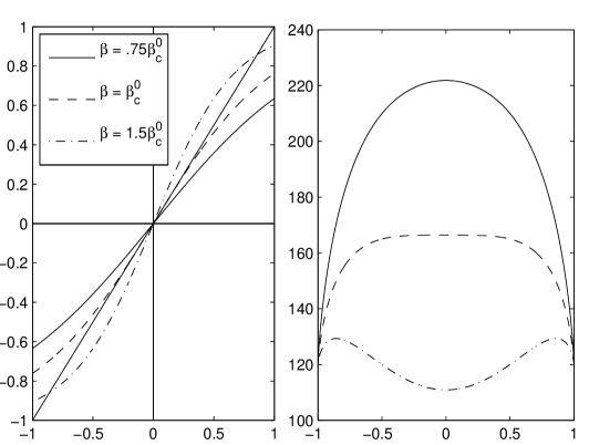
Figure 1: Left: The LHS and RHS for several values of $\beta$ of equation $(\ref{poleq})$. Right: Corresponding plots of the free energy. For all plots $\Omega=0$.

For $\beta<\beta_{c}^{0}<0$ there exist non-zero maximizers of the free energy $\sigma^{-}<0$, $\sigma^{+}>0$; the tanh function is odd, thus $\sigma^{-}=-\sigma^{+}$(figure (1)). The free energy is symmetric here so we need only consider fixed points $\sigma^{+}$ and $\sigma=0$. Consider the Taylor series of the free energy around zero

$$0 < \Phi(\sigma)-\Phi(0)$$ (31)

$$= (K+2\pi Tk_{B})\sigma^{2}+\frac{4\pi}{3}Tk_{B}\sigma^{4}+O\left(\sigma^{6}\right)$$ (32)

We therefore have a polarized ordered state for $\beta<\beta_{c}^{0}<0,$ which corresponds to solid-body rotating flow. A standard symmetry-breaking phase transition is thus predicted by the fixed point equation in this Bragg mean field model, in agreement with both the simple mean field theory [19] and Lim’s spherical model [12], [5], [15], [1], [4].
We have established the result,

Proposition 1: In the non-rotating case of the Bragg model, there is a negative temperature phase transition to a solid-body-rotating ordered state for $\beta<\beta_{c}^{0}=-2\pi/K<0.$ For all other values of the temperature - positive and negative - the most probable state is a mixed vorticity state.

Rotating

In the rotating regime the free energy can be approximated by a series as

$$\Psi_{T,\Omega}\left(\sigma\right)=-4\pi Tk_{B}\ln{2}+2\Omega\sigma+\left(K+2\pi Tk_{B}\right)\sigma^{2}+\frac{\pi Tk_{B}}{3}\sigma^{4}+O\left[\sigma^{6}\right]$$ (33)

For $\Omega>0$, and independent of whether the temperature is positive or negative, the RHS of the fixed point equation $(\ref{poleq})$ is zero at

$$\bar{\sigma}_{1}=\frac{-2\pi\Omega}{K}<0,$$ (34)

since $K>0.$ Moreover, it is easy to see that the zero $\bar{\sigma}_{1}$ satisfies

$$-1<\bar{\sigma}_{1}<0$$ (35)

if and only if planetary spin $\Omega$ - taken to be non-negative by convention - satisfies the condition

$$0<\Omega<\Omega_{cc}=\frac{K}{2\pi}$$ (36)

where $\Omega_{cc}>0$ is independent of temperature - that is, planetary spins are not too large. This condition turns out to be significant for the determination of the fixed points of $(\ref{poleq})$ in the rotating case which separates naturally into positive and negative temperature subcases considered next.

6.0.1 Positive temperatures

In the case of positive temperatures, by virtue of the property that the RHS of $(\ref{poleq})$ is decreasing in $\sigma_{1}$ and the fact that it is bounded between $\pm 1,$ there is always a fixed point $\sigma_{1}$ of $(\ref{poleq})$ satisfying

$$-1<\sigma_{1}<0.$$

By virtue of the shape of the graph of RHS of $(\ref{poleq}),$ this fixed point also satisfies

$$\bar{\sigma}_{1}<\sigma_{1}<0.$$ (37)

Furthermore, as $\beta\rightarrow\infty$, $\sigma_{1}\searrow\max{\left(\bar{\sigma}_{1},-1\right)}$. Since the zero $\bar{\sigma}_{1}$ satisfies

$$-1/2<\bar{\sigma}_{1}<0$$ (38)

if the planetary spin $\Omega$ is smaller than the threshold value

$$\Omega_{c}=\frac{K}{4\pi}>0,$$ (39)

we deduce from equation (37) that the fixed point also satisfies

$$-1/2<\sigma_{1}<0$$ (40)

for planetary spins smaller than $\Omega_{c}.$ From the fixed point equation(30) we find a phase transition where $\sigma<-1/2$ at positive critical temperature

$$T^{+}\left(\Omega\right)k_{B}=\frac{4\pi\Omega-K}{2\pi\ln{3}}$$

Thus, because $\Omega_{c}$ is independent of the inverse temperature $\beta>0,$ we have established the following result where we have taken the cutoff $|\sigma_{1}|=1/2$ to separate mixed states from ordered states,

Proposition 2:  (a) The most probable state in the Bragg model is the mixed vorticity state for all positive temperatures when planetary spins are smaller than $\Omega_{c}$ - there are therefore no phase transitions in positive temperatures in this case. (This is shown in figure (5) where the fixed points are plotted vs $T$ for very small $\Omega<\Omega_{c}.)$ (b) On the other hand for planetary spins that are not small, that is

$$\Omega\geq\Omega_{c}=\frac{K}{4\pi},$$ (41)

the fixed point $\sigma_{1}(\beta)\in(-1,0)$ has continuously increasing long range order as temperature decreases (see figure 4 below) and below$T_{c}^{+}(\Omega)>0,$ the statistical equilibria $\sigma_{1}<-1/2$ is an organized counter-rotating physical flow.

This is in agreement with the result obtained in the simple mean field approach in the case of positive temperatures [19]. Properties of the first threshold value of planetary spin are clearly shown in figure (2) and figure 3 where fixed points and free energy respectively are plotted vs $T$ for planetary spin $\Omega=\Omega_{c}$.

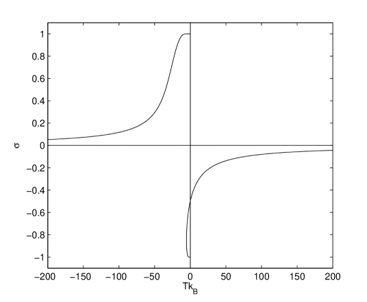
Figure 2: A graph of $\sigma$ vs $Tk_{B}$ when $\Omega=\Omega_{c}$.

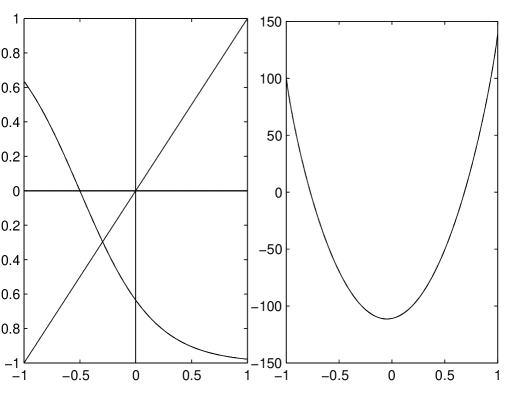
Figure 3: LEFT: A graph of the fixed point when $\beta>0,\Omega=\Omega_{c}$. RIGHT: The free energy

6.0.2 Transition between positive and negative temperatures with large $|T|$

For all values of planetary spins $\Omega,$ the most probable state changes smoothly through mixed states between high positive temperatures $T\gg 1$ and large-absolute-valued negative temperatures $T\ll-1$. At $T\gg 1,$ the preferred mixed state or fixed point has a slight negative angular momentum - it is slightly anti-rotating. For $T\ll-1,$ it is the reverse - the fixed point is a mixed state with a slight positive angular momentum or pro-rotation bias. These facts are clearly shown in figures (4) and (5) for several distinct values of $\Omega.$

6.0.3 Negative temperatures

We divide the analysis for negative temperatures into two natural categories - where the fixed point equation has the possibility of multiple fixed points and where it always have exactly one fixed point. In both categories, as negative $T$ increases (or decreases in absolute value), and for all values of planetary spin, the slightly pro-rotating mixed state described in the last subsection gives way continuously to a strongly pro-rotating state at $\beta^{-}(\Omega)<0$ - this is chosen to be the value of $\beta$ for which the fixed point $\sigma_{1}(\beta^{-})=0.5.$ This is clearly depicted in figures 2, 4 and 5 for several values of the planetary spin.

Solving (30) for $Tk_{B}$ gives

$$Tk_{B}=\frac{2\pi\Omega+\sigma K}{\pi\ln\left(\frac{1-\sigma}{1+\sigma}\right)}.$$ (42)

Thus,

$$\beta^{-}(\Omega)=\frac{-2\pi\ln{3}}{4\pi\Omega+K}$$ (43)

However, figures 2, (4) and (5) also indicate that there is another temperature threshold when the spin is not too large, namely

$$\beta_{c}^{\Omega}<0$$ (44)

where $\beta_{c}^{\Omega}$ $<0$ is the value for which multiple fixed points appear when $\beta\leq\beta_{c}^{\Omega}$ and when $\Omega<\Omega_{cc}$ - both defined below. We can find an estimate for $\beta_{c}^{\Omega}$. Critical value leading to the apearance of two more counter-rotating solutions of (30) is given by

$$0=\frac{dTk_{B}}{d\sigma}=\frac{K\left(1-\sigma^{2}\right)\ln\left(\frac{1+\sigma}{1-\sigma}\right)+4\pi\Omega+\sigma 2K}{\pi\left(1-\sigma^{2}\right)\left(\ln\left(\frac{1-\sigma}{1+\sigma}\right)\right)^{2}}$$ (45)

from which it follows

$$\beta_{c}^{\Omega}=\frac{-2\pi}{K\left(1-\sigma^{2}\right)}|_{\sigma=\sigma^{\Omega}}$$ (46)

An approximation of the numerator on the RHS of 45 by a third order polynomial in $\sigma$ gives

$$\sigma^{\Omega}\approx-\left(\frac{3\pi\Omega}{K}\right)^{1/3}$$ (47)

We can now conclude that

Lemma 3: The critical temperature$T_{c}^{\Omega}$ is increasing in $\Omega$

Proof: Follows imeadiately from (46) and (47)

One fixed point

In the case of negative temperatures, the physical bound $|\sigma_{1}|\leq 1,$ in the fixed point equation implies that there is another threshold on the planetary rotational rate. When

$$\Omega\geq\Omega_{cc}=\frac{V_{1}(K_{11}-K_{12})}{L_{1}}=2\Omega_{c},$$ (48)

there are only pro-rotating solutions $\sigma_{1}>0$ to the fixed point equation because any negative fixed point $\sigma_{1}^{-}<0$ - if they exist - must satisfy

$$\sigma_{1}^{-}<\bar{\sigma}_{1}<0$$

where the zero $\bar{\sigma}_{1}$ must in turn satisfy

$$\bar{\sigma}_{1}<-1$$

in view of (35) and (36), which leads to the contradiction $\sigma_{1}^{-}<-1.$ This is depicted in figure (4) for $\Omega>\Omega_{cc}.$

Thus, we have the result,

Proposition 4:  For large spins $\Omega>\Omega_{cc},$ there is a single negative- temperature transition at $\beta^{-}(\Omega)<0$ between the mixed and the strongly pro-rotating state for $|T|\ll 1.$

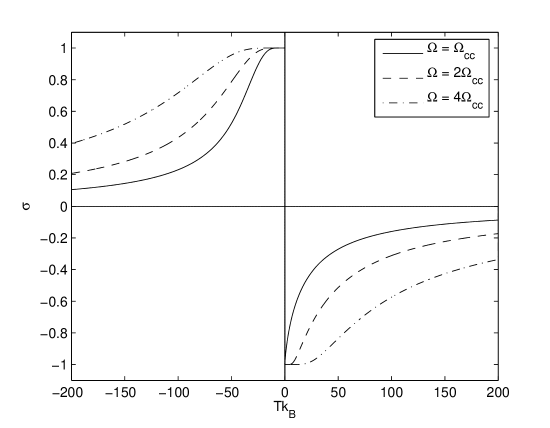
Figure 4: A graph of $\sigma$ vs $Tk_{B}$ when $\Omega>\Omega_{cc}$

Multiple fixed points

On the other hand, when $\Omega<\Omega_{cc},$ it is possible for the argument of tanh to be zero at values of $\bar{\sigma}_{1}$ within the physical range $-1<\bar{\sigma}_{1}<0,$ making it in turn possible to have counter-rotating or mixed- state fixed points that satisfy

$$-1\leq\sigma_{1}<\bar{\sigma}_{1}<0$$

if in addition,

$$\beta\leq\beta_{c}^{\Omega}<0.$$

In the case $\Omega\leq\Omega_{cc},$ and $\beta\leq\beta_{c}^{\Omega},$ there are generically three fixed points due to the structure of tanh, one pro-rotating and in general two others - one of which is strongly counter-rotating and one mixed with a small counter-rotation - which merge into a single degenerate counter-rotating / mixed solution when $\beta=\beta_{c}^{\Omega}$. This last threshold $\beta_{c}^{\Omega}<0$ is a consequence of the fact that $-\beta$ determines the slope of tanh near $0$ and a large enough slope is required in order for the graph of tanh to intersect the line of the identity function.

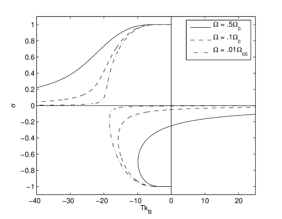
Figure 5: A graph of $\sigma$ vs $Tk_{B}$ when $\Omega_{c}>\Omega>0$.

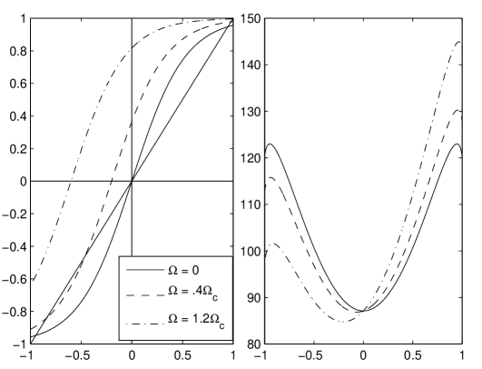
Figure 6: LEFT:Plots of the fixed points RIGHT: The free energy. Both plots are for the same value of $\beta<\beta_{c}^{\Omega}<0$

There is a transition at $\beta^{-}(\Omega)<0$ between the mixed and the strongly pro-rotating state and another negative temperature transition $\beta_{c}^{\Omega}<0$ when $\Omega<\Omega_{cc}$ where aditional critical points arise in (33). The Bragg free energy has a simple form in this case which we can exploit to easily see that the pro-rotating solution has greater free energy than the counter rotating solution in negative temperatures close to zero, as depicted in figure 6 for $\beta>\beta_{c}^{\Omega}.$

In the two domain case, $\Omega>0$ adds a linear term to the free energy functional,

$$\Psi_{T,\Omega}\left(\sigma\right)=\Psi_{T,0}\left(\sigma\right)+2\Omega\sigma$$ (49)

Recall from the nonrotating case that for $0>T>T^{0}_{c}$ the free energy has two maximizers we will denote here as $\bar{\sigma}^{-}$ and $\bar{\sigma}^{+}$; the free energy in this case is even so $\bar{\sigma}^{-}=-\bar{\sigma}^{+}$. Therefore, from Lemma 3 and equation (49),

$$\Psi_{T,\Omega}\left(\bar{\sigma}^{-}\right)<\Psi_{T,\Omega}\left(\sigma^{-}\right)<\Psi_{T,\Omega}\left(\bar{\sigma}^{+}\right)<\Psi_{T,\Omega}\left(\sigma^{+}\right)$$ (50)

It is also of interest to note that $\bar{\sigma}^{-}<\sigma^{-}<0<\bar{\sigma}^{+}<\sigma^{+}.$ In physical terms this implies that the ordered state $\sigma_{1}^{+}>0$ (in which positive relative vorticity dominates the northern hemisphere), is ‘more ordered’ than the symmetric solutions at $\Omega=0$ which is in turn more ordered than the counter-rotating fixed point $\sigma_{1}^{-}<0.$ We have demonstrated

Proposition 5:  For spins not too large, that is if $\Omega\leq\Omega_{cc},$ then for hottest inverse temperature such that $\beta<\beta_{c}^{\Omega}<0,$ there are exactly three fixed points in the Bragg model but the most probable state is pro-rotating such that $\sigma_{1}\nearrow 1.$

6.1 Summary of main results

In summary, the simple two domains case of the fixed point equation predicts that in the rotating problem, there are two critical values of the planetary spin, $\Omega_{c}$ in (39) and $\Omega_{cc}=2\Omega_{c}.$ Below $\Omega_{c}$, there is no transition at positive temperatures and the most probable barotropic flow state is mainly a mixed state (40) with some small amount of counter-rotation which vanishes as temperature increases. For planetary spins above $\Omega_{c},$ there is a continuous positive temperature transition from mixed states at $T>T_{c}^{+}(\Omega)$ to strongly counter-rotating barotropic states at lower positive temperatures.

For all values of spin, there is a smooth transition through mixed states at $\beta=0$ between slightly anti-rotating mixed states for $T\gg 1$ and slightly pro-rotating mixed states for negative $T$ with $|T|\gg 1.$ Again for all values of spin $\Omega$, there is a continuous transition at $\beta^{-}(\Omega)<0$ between mixed states for cooler negative $\beta>\beta^{-}(\Omega)$ and strongly pro-rotating states for hotter $\beta<\beta^{-}(\Omega).$ For large spins $\Omega>\Omega_{cc},$ this is the only possible transition at negative temperatures.

For intermediate to small values of spin, $\Omega<\Omega_{cc},$ there is a negative threshold $\beta_{c}^{\Omega}$ at which the possibility for multiple (meta-stable) thermodynamic equilibria first arises. We argued that when there are multiple fixed points, the pro-rotating branch has the largest free energy and thus continues to be the thermodynamically stable macrostate. We conclude that for all spins, there is a single negative- temperature- transition at $\beta^{-}(\Omega)<0$ to the pro-rotating state for the hottest negative temperatures - those with the smallest absolute values corresponding to the largest kinetic energy.

The complete analysis of the transitions in the non-rotating case and in the rotating case agrees well with the simple mean field theory and Lim’s spherical model.

7 The infinite dimensional nonextensive limit

As noted above, the model does not have an extensive limit from which we can derive intensive quantities. We have therefore bypassed the standard thermodynamic construction and directly built an non-extensive model. Convergence theorems support our continuum model. In this frame work we have had no need to include stipulations on the types configuration of domains. In light of this, we will consider a sequence of domain systems which are constructed from Voronoi cells of a uniform mesh as in Lim and Nebus[15]. This affords us an advantage that we may assume the coarse grained domains to be spatially symmetric. We henceforth refer to the sequence of domain systems and their associated ensembles as a Bragg process. The limiting ensemble of a Bragg process is the space $L_{2}(S^{2})$ of functions $\sigma:S^{2}\mapsto\left[-1,1\right]$, which has an expression of the free energy analogous to the discrete case,

$$\Psi\left[\sigma\right]=-\frac{1}{2}\int dx\int dy\sigma(x)\sigma(y)K(x,y)-\Omega\int dx\sigma(x)L(x)$$

$$+Tk_{B}\int dx\left[\frac{1+\sigma(x)}{2}\ln\frac{1+\sigma(x)}{2}+\frac{1-\sigma(x)}{2}\ln\frac{1-\sigma(x)}{2}\right]$$

from which we can easily recover the fixed point equation. The free energy must be extremized over the subspace of functions constrained by Stokes’ theorem $\Sigma=\left\{\sigma:S^{2}\mapsto[-1,1]|0=\int_{S^{2}}dx\sigma(x)\right\}$. Another physical constraint namely bounded relative enstrophy - the square of the $L_{2}$ norm of the coarse-grained relative vorticity field $\sigma(x)$ - is implicit in the condition that $|\sigma|\leq 1$ in the fixed point equation which can be derived in the continuous case similarly to the above discrete case,

$$\sigma(x)=\tanh{\left[\beta(\Omega L(x)+\lambda)+\beta\int_{S^{2}}dy\sigma(y)K(x,y)\right].}$$ (51)

It is clear from the definition of $K$ (16) that we have recovered the inverse Laplacian $G$ and we can rewrite (51) as

$$\Delta\psi=\tanh{\left[\beta\left(\Omega L(x)+\lambda+\psi\right)\right]}$$ (52)

where $\psi$ is the course grained stream function. From this form, remembering that $L(x)$ is proportional to the first spherical harmonic and $\left\langle\Delta\psi\right\rangle=0$ we see that $\lambda=0$. Indeed, for any $\psi$ we have $\lambda=0$ implies $\left\langle\tanh{\left[\beta\left(\Omega L(x)+\lambda+\psi\right)\right]}\right\rangle=0$ and,

$$\frac{d}{d\lambda}\left\langle\tanh{\left[\beta\left(\Omega L(x)+\lambda+\psi\right)\right]}\right\rangle\\ =\left\langle\frac{d}{d\lambda}\tanh{\left[\beta\left(\Omega L(x)+\lambda+\psi\right)\right]}\right\rangle$$

$$=\left\langle\beta\cosh^{-2}{\left[\beta\left(\Omega L(x)+\lambda+\psi\right)\right]}\right\rangle$$

serves to show the average is monotonic in $\lambda$.

While the original discrete model was limited in its degrees of freedom, we now have a continuum of freedom for the spin since now the coarse-grained state is given by a bounded function $\sigma(x)$ in $L_{2}(S^{2})$ with zero circulation $\int_{S^{2}}dx\sigma(x)=0$. Further the Bragg estimation of interaction energy became very accurate in the continuum model. The price paid, like in all mean field models, is the artifact of the entropy estimation. However, the Shannon entropy of a binary variable is exactly what enables our derivation of the tanh fixed point equation above. The figure below shows the spin states of some thermodynamic regimes obtained numerically.

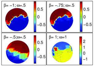
Figure 7: Some fixed point solutions

8 Conclusion

In conclusion it must be emphasized that the combined angular momentum of the fluid and solid sphere is conserved even when that of the fluid alone is not. Similarly, without loss of generality for the purposes here, we can assume that the complex torque mechanism responsible for coupling fluid to sphere is conservative, and thus, the combined energy of the fluid-sphere system is conserved.

In taking the mass of the rotating sphere to be infinite here and in [12], [5], we have essentially modeled the statistical mechanics of the coupled fluid-sphere problem as one having separate reservoirs for angular momentum and energy. It was shown in [12] and [19] that the particular form of the kinetic energy functional for coupled barotropic flow on a sphere allows us to conveniently combine these two reservoirs into one so there is only one inverse temperature $\beta.$ Introducing a distinct reservoir for angular momentum, that is, imposing a separate canonical constraint on the angular momentum of the fluid will not change the physics but will add to the clutter in the resulting model.

We remark here that a series of experiments on decaying and forced-damped (or stationary) quasi-2D turbulence in square domains with no-slip and stressless boundaries - see [7] and references therein - have highlighted the role of variable angular momentum in inverse cascades to self-organized structures. In particular, normal forces at the boundary of the square can in principle produce a torque without requiring shear or the presence of friction at the boundary. This conservative mechanism for angular momentum transfer between fluid and boundary - despite the obvious mismatch in geometry - provides the best experimental comparison that we know to the (unresolved) torque mechanism introduced and developed by the first author into the coupled fluid-sphere statistical mechanics models in a series of recent papers.

For a more detailed view of the complex torque mechanism that couples the fluid to the rotating sphere, one will have to invoke the observed and theorized fact that a baroclinic component of the fluid forms Hadley cells driven by non-uniform solar insolation which in turn serves to transfer high momentum fluid in the equatorial region up to the middle atmosphere and mid-latitudes. The planetary boundary layer is a very complex region that is responsible for transferring the solid sphere’s angular momentum to the fluid as it flows towards the equator from mid-latitudes and the fluid’s angular momentum to the sphere between the polar region and mid-latitudes. Any attempt to model this torque mechanism explicitly will result in technical difficulties that can only be resolved by a huge computational effort. Fortunately, the very essence of statistical mechanics - namely coarse-graining - allows us to formulate a viable theory without explicitly resolving this complex torque mechanism.

The results derived by using Bragg’s method are in good agreement with those found through Monte - Carlo simulations of the spherical energy-enstrophy model by Ding and Lim [1], [4] and with a simple mean field theory [19], in the non-rotating, rotating positive temperature and possibly rotating negative temperature problems. More details can be found in the recent book [11] and on the website http://www.rpi.edu/~limc. Further work should be done, however, to refine the multi-dimensional Bragg method and extend it to more complex geophysical flows such as shallow water flows coupled to a rotating sphere. The infinite-dimensional fixed point formulation in the previous section gave us an interesting nonlinear elliptic equation (52) that should be further analyzed. Complementing the work here, the first author recently presented exact solutions to the spherical model for the energy-relative enstrophy theory of the coupled barotropic fluid-sphere system [12], [5].

Acknowledgement
This work is supported by ARO grant W911NF-05-1-0001 and DOE grant DE-FG02-04ER25616.

References

- [1] Xueru Ding and Chjan Lim. Equilibrium phases in a energy- relative enstrophy statistical mechanics model of barotropic flows on a rotating sphere – non- conservation of angular momentum. American Meteorological Society Proceedings, 2006.
- [2] Kerson Huang. Statistical Mechanics Second Edition. John Wiley & Sons, 1988.
- [3] C.C. Lim, Energy extremals and nonlinear stability in an Energy-relative enstrophy theory of the coupled barotropic fluid - rotating sphere system, J. Math Phys. 48(1), 1-21, 2007.
- [4] X. Ding and C.C. Lim, Phase transitions to super-rotation in a coupled Barotropic fluid - rotating sphere system, Physica A 374, 152-164, 2007.
- [5] C.C. Lim, Phase transitions to Super-rotation in a Coupled Fluid - Rotating Sphere System, Proc. IUTAM Symp., Steklov Institute, Moscow, August 2006 (http://www.rpi.edu/~limc/IUTAM06.pdf).
- [6] S.R.Maassen, H. Clercx, and G. van Heijst, Self-organisation of decaying quasi-2D turbulence in stratified fluid in rectangular containers, J Fluid Mech. 495, 19-33, 2003.
- [7] G. van Heijst, H. Clercx, and D. Molenaar, The effects of solid boundaries on confined 2d turbulence, J. Fluid Mech., 554, 411-431, 2006.
- [8] T.S. Lundgren and Y.B. Pointin, Statistical mechanics of 2D vortices, J. Stat Phys. 17, 323 - , 1977.
- [9] J. Miller, Statistical mechanics of Euler equations in two dimensions, Phys. Rev. Lett. 65, 2137-2140 (1990).
- [10] R. Robert and J. Sommeria, Statistical equilibrium states for two-dimensional flows, J. Fluid Mech., 229, 291-310, 1991.
- [11] C.C. Lim and J. Nebus, Vorticity, Statistical Mechanics and Monte-Carlo Simulations, Springer-Verlag New York 2006.
- [12] C.C. Lim, A spherical model for a coupled barotropic fluid - rotating solid sphere system - exact solution, preprint 2006.
- [13] L. Onsager, Statistical Hydrodynamics, Nuovo Cimento Suppl. 6 (1949) 279-289.
- [14] Chjan Lim. Energy maximizers, negative temperatures, and robust symmetry breaking in vortex dynamics on a nonrotating sphere. SIAM, 65(6):2093-2106, 2005.
- [15] Chjan Lim and Joseph Nebus. The spherical model of logarithmic potentials as examined by monte carlo analysis. Physics of Fluids, 16:4020–4027, 2004.
- [16] J.S. Frederiksen and B.L. Sawford, Statistical dynamics of 2D inviscid flows on a sphere, J. Atmos Sci 31, 717-732, 1980.
- [17] R.H. Kraichnan, Statistical dynamics of two-dimensional flows, J. Fluid Mech. 67, 155-175 (1975).
- [18] H. E. Stanley, Introduction to phase transitions and critical phenomena, Oxford University Press, New York, 1971.
- [19] C.C. Lim, Extremal free energy in a simple Mean Field Theory for a Coupled Barotropic fluid - Rotating Sphere System,, accepted by DCDS-A 2006.