New critical behavior in unconventional ferromagnetic superconductors

Abstract

New critical behavior in unconventional superconductors and superfluids is established and described by the Wilson-Fisher renormalization-group method. For certain ordering symmetries a new type of fluctuation-driven first order phase transitions at finite and zero temperature are predicted. The results can be applied to a wide class of ferromagnetic superconducting and superfluid systems, in particular, to itinerant ferromagnets as UGe₂ and URhGe.

I INTRODUCTION

In this paper new critical behavior in unconventional ferromagnetic superconductors and superfluids is established and described. This behavior corresponds to an isotropic ferromagnetic order in real systems but does not belong to any known universality class Uzunov:1993 and, hence, it could be of considerable experimental and theoretical interest. Due to crystal and magnetic anisotropy, a new type of fluctuation-driven first order phase transitions occur, as is shown in the present investigation. The novel fluctuation effects can be observed near finite and zero temperature (“quantum”) phase transitions Uzunov:1993 ; ShopovaPR:2003 in wide class of ferromagnetic systems with unconventional (spin-triplet) superconductivity or superfluidity.

The present study has been performed on the special example of intermetallic compounds UGe₂ and URhGe, where the remarkable phenomenon of coexistence of itinerant ferromagnetism and unconventional spin-triplet superconductivity Sigrist:1991 has been observed Saxena:2000 . For example, in UGe₂, the coexistence phase occurs Saxena:2000 at temperatures $0\leq T<1$ K and pressures $1<P<P_{0}\sim 1.7$ GPa. A fragment of ($P,T$) phase diagrams of itinerant ferromagnetic compounds Saxena:2000 is sketched in Fig. 1, where the lines $T_{F}(P)$ and $T_{c}(P)$ of the paramagnetic(P)-to-ferromagnetic (F) and ferromagnetic-to-coexistence phase (C) transitions are very close to each other and intersect at very low temperature or terminate at the absolute zero ($P_{0},0$). At low temperature, where the phase transition lines are close enough to each other, the interaction between the real magnetization vector $\mbox{\boldmath$M$}(\mbox{\boldmath$r$)}=\{M_{j}(\mbox{\boldmath$r$});j=1,...,m\}$ and the complex order parameter vector of the spin-triplet Cooper pairing Sigrist:1991 , $\psi(\mbox{\boldmath$r$})=\{\psi_{\alpha}(\mbox{\boldmath$r$})=(\psi^{\prime}_{\alpha}+i\psi_{\alpha}^{\prime\prime});\alpha=1,....n/2\}$ ($n=6$) cannot be neglected Uzunov:1993 and, as shown here, this interaction produces new fluctuation phenomena.

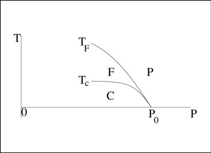
Figure 1: ($P,T$) diagram with a multicritical point $(P_{0},T\sim 0)$ at very low temperature. Para- (P), ferromagnetic (F), and coexistence (C) phases, separated by the lines $T_{f}(P)$ and $T_{c}(P)$ of P-F and F-C phase transitions, respectively.

Both thermal fluctuations at finite temperatures ($T>0$) and quantum fluctuations (correlations) near the $P$–driven quantum phase transition at $T=0$ should be considered but at the first stage one may neglect the quantum effects ShopovaPR:2003 as irrelevant to finite temperature phase transitions ($T_{F}\sim T_{c}>0$). The present treatment of recently derived free energy functional Machida:2001 by the standard Wilson-Fisher renormalization group (RG) Uzunov:1993 shows that unconventional ferromagnetic superconductors with isotropic magnetic order ($m=3$) exhibit a quite particular multi-critical behavior for any $T>0$, whereas the magnetic anisotropy ($m=1,2$) generates fluctuation-driven first order transitions (see Sec. III and IV).

As shown in Sec. II certain terms in the general free energy Hamiltonian Shopova:2003 , which are relevant for the mean-field analysis Machida:2001 ; Shopova:2003 become irrelevant within the RG framework. This leads to a considerable simplification of the RG treatment but on the other side specific symmetry properties of the relevant Hamiltonian terms make the same RG treatment quite nontrivial (Sec. III). The RG study is performed by the known $\epsilon$-expansion (see, e.g., Ref. Uzunov:1993 ).

A particular feature of the present theoretical consideration is the breakdown of usual $\epsilon$-expansion in the one-loop approximation for RG equations $(\epsilon=6-d)$. Thus, the latter cannot yield conclusive results and one is forced to derive the two-loop RG equations. The higher order of the theory restores the $\epsilon$-expansion in a modified form - expansion in non-integer powers ($\epsilon^{1/4},\epsilon^{1/2},\dots$) of $\epsilon$. In the framework of two-loop RG equations one obtains the above mentioned new critical behavior.

This theoretical scenario looks quite similar to the breakdown of the usual $\epsilon$-series and the ${\tilde{\epsilon}}$-expansions in non-integer powers of ${\tilde{\epsilon}}=(4-d)$, known for the first time from the theory of critical phenomena in anisotropic disordered systems (see, e.g., Ref. Lawrie:1987 ). It should be emphasized that the mentioned similarity between the present theoretical analysis and that in certain disordered systems cannot be extended beyond some general features of the $\epsilon$-expansions. The mechanism leading to the ${\tilde{\epsilon}}=(4-d)$-expansion in non-integer powers of ${\tilde{\epsilon}}$ in anisotropic disordered systems is quite different from the mechanism revealed here. The latter is a result of the particular symmetry of the interaction between the fields $\psi$ and $M$.

In order to re-derive the results in Sec. III, one should carefully take into account all the relevant dependencies of the perturbation integrals on the parameters of the theory. For this reason here the relevant perturbation contributions to the Hamiltonian vertex parameters are presented in a general form. In certain cases, the perturbation integrals are calculated for zero values of the external wave vectors, or, for zero values of certain Hamiltonian parameters Uzunov:1993 ; Aharony:1974 . In such cases some of the integrals give equal contributions to the respective RG equations, but in other cases, for example, the investigation of the RG stability matrix, one should carefully take into account all the differences in the contributions of the same integrals. The calculation of elements of the linearized RG stability matrix is made through the exact dependence of the perturbation terms on the parameters of the Hamiltonian and for this aim one needs to know the perturbation integrals in their initial general form. In all other aspects, the present consideration follows the standard prescriptions, described in Ref. Aharony:1974 and applied to the study of complex systems by means of RG and $\epsilon$-expansions in non-integer power of $\epsilon$ (see, e.g., Ref. Lawrie:1987 ). In spite of the specific features of the present analysis, it does not contradict to the usual concepts and interpretations of $\epsilon$-series (see, e.g., Ref.  Lawrie:1987 ). In this paper some integrals appear for the first time in the RG theory of complex systems. These integrals together with known ones are evaluated to the accuracy needed for the RG analysis in two-loop approximation (See Sec. III). In RG studies in higher orders of the loop expansion some additional relevant terms of the same integrals should be calculated and used. In order to facilitate the reproducibility of the results and further investigations, some details of the calculations and an extended discussion of the most important stages of the RG investigation are presented (Sec. III and IV).

These remarks are important throughout the RG analysis: (1) the calculation of fixed point (FP) coordinates, (2) the calculation of elements of the RG stability matrix, and (3) the calculation of critical exponents, including the stability ones. Besides, the derivation of the RG equations should be made with a considerable attention for reasons explained in Sec. III. Note, that the RG investigation can be performed in an alternative way, namely, the RG can be applied to a new effective Hamiltonian, which is a functional of the $\psi$-field only. This point is briefly discussed in Sec. II.

The consideration of quantum effects exhibits for the first time an example of a complex quantum criticality characterized by a double-rate quantum critical dynamics (Sec. III.E). In the quantum limit ($T\rightarrow 0$) the fields $M$ and $\psi$ have different dynamical exponents, $z_{M}$ and $z_{\psi}$, and this leads to two different upper critical dimensions: $d_{U}^{\psi}=6-z_{\psi}$ and $d_{U}^{M}=6-z_{M}$. For this reason the more complete theoretical description of quantum effects on the properties of the zero-temperature (multi)critical point meets difficulties (Sec. III.E and Sec. V). The treatment of spin-triplet ferromagnetic superconductors with magnetic anisotropies ($m<3$) and/or crystal symmetry lower than the cubic one requires a somewhat different RG analysis. These systems are considered in Sec. IV. In Sec. V the main results are summarized and discussed.

II EFFECTIVE HAMILTONIAN

Relevant part of the fluctuation Hamiltonian of unconventional ferromagnetic superconductors Machida:2001 ; Shopova:2003 can be written in the form

$${\cal{H}}=\sum_{\mbox{\boldmath$k$}}\left[\left(r+k^{2}\right)|\psi(\mbox{\boldmath$k$})|^{2}+\frac{1}{2}\left(t+k^{2}\right)|\mbox{\boldmath$M$}(\mbox{\boldmath$k$})|^{2}\right]+\frac{ig}{\sqrt{V}}\sum_{\mbox{\boldmath$k$}_{1},{\mbox{\boldmath$k$}_{2}}}{\mbox{\boldmath$M$}}\left({\mbox{\boldmath$k$}}_{1}\right).\left[\psi\left({\mbox{\boldmath$k$}}_{2}\right)\times\psi^{\ast}\left({\mbox{\boldmath$k$}}_{1}+{\mbox{\boldmath$k$}}_{2}\right)\right]$$ (1)

where $V\sim L^{d}$ is the volume of the $d-$dimensional system, the length unit is chosen so that the wave vector $k$ is confined below unity ($0\leq k=|{\mbox{\boldmath$k$}}|\leq 1)$, $g\geq 0$ is a coupling constant, describing the effect of the scalar product of $M$ and the vector product $(\psi\times\psi^{\ast})$ for symmetry indices $n/2=m=3$, and the parameters $r=\alpha_{s}(T-T_{s})$ and $t=\alpha_{f}(T-T_{f})$ are expressed by the critical temperatures of the generic ($g\equiv 0$) superconducting ($T_{s}$) and ferromagnetic ($T_{f}$) transitions (as usual, the parameters $\alpha_{s}$ and $\alpha_{f}$ are positive). As mean field studies indicate Machida:2001 ; Shopova:2003 , $T_{s}(P)$ is much lower than $T_{c}(T)$ and $T_{F}(P)\neq T_{f}(P)$. As shown below the Hamiltonian (1) describes the main fluctuation effects in a close vicinity of critical points in spin-triplet ferromagnetic superconductors. It is convenient to choose units, in which $k_{B}=1$, and the upper cutoff for the magnitude $k=|\mbox{\boldmath$k$}|$ of the wave vectors in Eq. (1) is equal to unity. Some perturbation expansions within the RG investigation, in particular, those for isotropic systems ($n/2=m=3$) can be performed with the help of known representation $\varepsilon_{j\alpha\beta}$ of the components $(\psi\times\psi^{\ast})_{j}$ of the respective vector product in Eq. (1).

The fourth order terms ($M^{4},|\psi|^{4},M^{2}|\psi|^{2}$) in the total free energy (Hamiltonian) Machida:2001 ; Shopova:2003 have not been included in Eq. (1) as they are irrelevant to the present investigation. The simple dimensional analysis shows that the $g-$term in Eq. (1) corresponds to a scaling factor $b^{3-d/2}$ and, hence, becomes relevant below the upper borderline dimension $d_{U}=6$, whereas fourth order terms are scaled by a factor $b^{4-d}$ as in the usual $\phi^{4}-$theory and are relevant below $d<4$ ($b>1$ is a scaling number) Uzunov:1993 . Therefore, we should perform the RG investigation in spatial dimensions $d=6-\epsilon$, where the $g$–term in Eq. (1) describes the only relevant fluctuation interaction. Besides, the total fluctuation Hamiltonian Machida:2001 ; Shopova:2003 contains off-diagonal terms of the form $k_{i}k_{j}\psi_{\alpha}\psi^{\ast}_{\beta}$; $i\neq j$ and/or $\alpha\neq\beta$. Using a convenient loop expansion these terms can be completely integrated out from the partition function to show that they modify the parameters ($r,t,g$) of the theory but they do not affect the structure of the model (1). So, such terms change auxiliary quantities, for example, the coordinates of the RG fixed points (FPs) but they do not affect the main RG results for the stability of the FPs and the values of the critical exponents. Here these off-diagonal gradient terms will be ignored.

The mean-field investigation of the total Hamiltonian shows that the $g$-term in Eq. (1) triggers the spin-triplet superconductivity ($M$-trigger mechanism Shopova:2003 ). The fourth order terms, mentioned above, do not play such a crucial role. They merely stabilize the ordered phases, provide a correct shape of the ($P,T$) phase domains for the specific crystal and magnetic symmetries. Neglecting these terms one looses the opportunity to describe the equilibrium order $\langle\mbox{\boldmath$M$}\rangle=\mbox{\boldmath$M$}-\delta\mbox{\boldmath$M$}$ and $\langle\psi\rangle=\psi-\delta\psi$, but as shown above, the main fluctuation effects in a close vicinity of the phase transition points can be totally taken into account. Here the attention is focussed on the behavior above the phase transition points where $\langle\mbox{\boldmath$M$}\rangle=\langle\psi\rangle=0$, and hence, $\mbox{\boldmath$M$}\equiv\delta\mbox{\boldmath$M$}$ and $\psi\equiv\delta\psi$.

The simplest theory with upper critical dimension $d_{U}=6$ is that of a classic scalar field $\varphi$ with $\varphi^{3}$-interaction (see, e.g., Ref. Uzunov:1993 ). Quite more complex problem, where $d_{U}=6$ and an expansions in powers of $\epsilon=(6-d)$ are used arises in the theory of tricritical Lifshitz points Uzunov:1993 ; Uzunov:1985 . In all these cases the upper critical dimension $d_{U}$ is determined by a simple dimensional analysis in the so-called tree approximation Uzunov:1993 and/or by a check of singularities of the relevant perturbation integrals (See Sec. III). The two mentioned examples are from theories of a single (vector or scalar) field whereas the present theory (1) describes two fields. Here the critical dimension $d_{U}=6$ is a result of the simple fact that the total power of fields in interaction ($g$-) term in Eq. (1) is equal to three. Thus one may suppose that some of the results in this paper could be applied to critical phenomena in improper ferroelectrics Gufan:1980 , where interactions of two fields ($\varphi_{1}$ and $\varphi_{2}$) of type $\varphi_{1}\varphi^{2}_{2}$ also occur and the upper critical dimension is $d_{U}=6$. The present investigation will demonstrate, however, that for such interaction of two fields and upper critical dimension $d_{U}=6$, the RG analysis can lead to different results depending on the specific symmetry of the interaction term. The outcomes are two: a lack of stable FPs and physical arguments leading to a prediction of first order phase transitions, or, the presence of a stable FP and, hence, a stable critical behavior. While the particular symmetry of interaction term provides a new stable FP and, hence, a new critical behavior for symmetry indices $n/2=m=3$, one cannot be certain that the same prediction can be made for ferroelectrics without a specific investigation.

One may consider several cases: (i) isotropic systems, namely, cubic crystal symmetry and isotropic magnetic order, when all field components $\psi_{\alpha}$ and $M_{j}$ can be different zero ($n/2=m=3$), (ii) anisotropic systems when the total number $(m+n/2)$ of field components is less than six. Note that the case (i) is of major interest to real systems, where fluctuations of all field components are possible, despite the presence of crystal and magnetic anisotropy that nullifies some of the equilibrium field components.

The functional integral over the fields $M_{j}(\mbox{\boldmath$k$})$ in the partition function $Z=\int D\psi\mbox{\boldmath$M$}\mbox{exp}(-H/T)$ can be exactly calculated, for example, by the total summation of perturbation series in powers of the interaction parameter $g$. In result, one will obtain a new effective Hamiltonian ${\tilde{H}}(\psi)$, which is a functional of a single field - $\psi$. In this new $\psi$-theory the effects of the magnetic ($M$-) subsystem will be “hidden” in the vertex parameters of ${\tilde{H}}(\psi)$. The effective Hamiltonian can also be treated by RG but this task is beyond the scope of the present consideration. The Hamiltonian (1) explicitly describes the fluctuations of the magnetization $M$ and this is the advantage with respect to ${\tilde{H}}(\psi)$.

Figure 2: One loop diagrammatic contributions to the re-normalized correlation functions $\langle|\psi_{\alpha}|^{2}\rangle$ and $\langle|M_{j}|^{2}\rangle$, and to the $g$-term in Eq. (1); ($\bullet$) represents the $g$-interaction, the thin legs represent $M_{j}(\mbox{\boldmath$k$})$, the tick legs with incoming and outcoming arrows stand for the field components $\psi_{\alpha}(\mbox{\boldmath$k$})$ and $\psi_{\alpha}^{\ast}(\mbox{\boldmath$k$})$, respectively; the internal thin and thick lines represent the bare correlation functions $\langle|\psi_{\alpha}|^{2}\rangle_{0}$ and $\langle|M_{j}|^{2}\rangle_{0}$, respectively.

Figure 3: Two loop diagrammatic contributions to the correlation function $\langle|\psi_{\alpha}(\mbox{\boldmath$k$})|^{2}\rangle$. The symbols have been explained in Fig. 2. The arrows of the thick lines have been omitted.

Figure 4: Two loop diagrammatic contributions to the correlation function $\langle|M_{j}(\mbox{\boldmath$k$})|^{2}\rangle$. The symbols have been explained in Fig. 2. The arrows of the thick lines have been omitted.

Figure 5: A sum of two loop diagrams of order $g^{5}$ with a zero contribution to the renormalization of the $g$-term in Eq. (1). The symbols have been explained in Fig. 2.

Figure 6: Two loop diagrammatic contributions to the $g$-term in Eq. (1). The arrows of the thick lines have been omitted.

III ISOTROPIC SYSTEMS

III.1 RG equations

Following Ref. Uzunov:1993 ; Aharony:1974 ; Lawrie:1987 here we derive the Wilson-Fisher RG equations for isotropic systems ($n/2=m=3$), described by the Hamiltonian (1), up to the two-loop order. The main results from the RG analysis of anisotropic systems $(n/2+m<6)$ can be obtained within the one-loop order and this point will be discussed in Sec. IV. The one loop contributions to the RG equations are shown by diagrams in Fig. 2. The two loop diagrammatic contributions to the renormalized correlation functions $\langle|\psi_{\alpha}(\mbox{\boldmath$k$})|^{2}\rangle$ and $\langle|M_{j}(\mbox{\boldmath$k$})|^{2}\rangle$ are shown in Fig. 3 and 4, respectively. Although the perturbation theory of the Hamiltonian (1) is developed in a standard way, i.e., by an expansion in powers of the interaction parameter $g$, the derivation of the two-loop terms in the RG equations is quite nontrivial because of the special symmetry properties of the interaction $g$-term. For example, some diagrams with opposite arrows of internal lines, as the couple shown in Fig. 5, have opposite signs and compensate each other. The terms bringing contributions to the $g$–vertex are shown diagrammatically in Fig. 6.

In Figs. (2) - (6) the thin external legs and thin internal lines, corresponding to the field components $M_{j}(\mbox{\boldmath$k$})$ and the bare correlation function $\langle|M_{j}(\mbox{\boldmath$k$})|^{2}\rangle_{0}$, respectively, can always be supplied with incoming and/or outcoming arrows as this has been made for the thick legs and lines, representing the fields $\psi_{\alpha}(\mbox{\boldmath$k$})$ and $\psi_{\alpha}^{\ast}(\mbox{\boldmath$k$})$, and the bare correlation function $\langle|\psi_{\alpha}(\mbox{\boldmath$k$})|^{2}\rangle_{0}$, respectively. The thin lines in Figs. (2) - (6) can take any orientation, because the magnetization $\mbox{\boldmath$M$}(\mbox{\boldmath$x$})$ is a real vector and, hence, the Fourier amplitudes of the field components, $M_{j}(\mbox{\boldmath$k$})$, obey the relation $M^{\ast}_{j}(\mbox{\boldmath$k$})=M_{j}(-\mbox{\boldmath$k$})$. In Figs. (2) - (6) the arrows of thin lines and legs are omitted but one should have in mind that in practical calculations with the help of these diagrams, arrows of any orientation can be used.

The RG equations have been derived in the following general form:

$$r^{\prime}=b^{2-\eta_{\psi}}\left\{r-2J_{sf}(r,t;0)g^{2}-2\left[2B_{1}(r,t,0)+2B_{2}(r,t,0)+B_{3}(r,t,0)\right]g^{4}\right\}$$ (2)

$$t^{\prime}=b^{2-\eta_{M}}\left\{t-2J_{ss}(r,r;0)g^{2}-2\left[A_{1}(r,t,0)+4A_{2}(r,t,0)\right]g^{4}\right\},$$ (3)

$$g^{\prime}=b^{3-d/2-\eta_{\psi}-\eta_{M}/2}\left\{g+J_{3}(r,t)g^{3}+\left[D_{1}(r,t)+4D_{2}(r,t)+2D_{3}(r,t)+2D_{4}(r,t)\right]g^{5}\right\},$$ (4)

$$b^{\eta_{\psi}}=1-2a_{sf}g^{2}-(2b_{1}+2b_{2}+b_{3})g^{4}$$ (5)

and

$$b^{\eta_{M}}=1-2a_{ss}g^{2}-2(a_{1}+2a_{2})g^{4}.$$ (6)

Here $b>1$ is a scaling number, $\eta_{\psi}$ and $\eta_{M}$ are the Fisher exponents (anomalous dimensions of the fields $\psi$ and $M$, respectively), and the perturbation integrals are given by

$$J_{sf}(r,t,\mbox{\boldmath$k$})=\int^{\prime}\frac{d^{d}p}{(2\pi)^{d}}\frac{1}{(p^{2}+t)\left[(\mbox{\boldmath$p$}+\mbox{\boldmath$k$})^{2}+r\right]},$$ (7)

$$J_{ss}(r,r,\mbox{\boldmath$k$})=J_{sf}(r,r,\mbox{\boldmath$k$}),$$ (8)

$$J_{3}(r,t)=\int^{\prime}\frac{d^{d}p}{(2\pi)^{d}}\frac{1}{(p^{2}+r)^{2}(p^{2}+t)},$$ (9)

$$A_{1}(r,t,\mbox{\boldmath$k$})=\int^{\prime}\frac{d^{d}p_{1}d^{d}p_{2}}{(2\pi)^{2d}}\frac{1}{(p^{2}_{1}+r)(p^{2}_{2}+r)\left[(\mbox{\boldmath$p$}_{1}-\mbox{\boldmath$p$}_{2})^{2}+t\right]\left[(\mbox{\boldmath$p$}_{1}+\mbox{\boldmath$k$})^{2}+r\right]\left[(\mbox{\boldmath$p$}_{2}+\mbox{\boldmath$k$})^{2}+r\right]},$$ (10)

$$A_{2}(r,t,\mbox{\boldmath$k$})=\int^{\prime}\frac{d^{d}p_{1}d^{d}p_{2}}{(2\pi)^{2d}}\frac{1}{(p^{2}_{1}+r)^{2}\left[(\mbox{\boldmath$p$}_{1}+\mbox{\boldmath$p$}_{2})^{2}+r\right]\left[(\mbox{\boldmath$p$}_{1}+\mbox{\boldmath$k$})^{2}+r\right]\left[(\mbox{\boldmath$p$}_{2}^{2}+t\right]},$$ (11)

$$B_{1}(r,t,\mbox{\boldmath$k$})=\int^{\prime}\frac{d^{d}p_{1}d^{d}p_{2}}{(2\pi)^{2d}}\frac{1}{(p^{2}_{1}+r)^{2}\left[(\mbox{\boldmath$p$}_{1}+\mbox{\boldmath$p$}_{2})^{2}+r\right]\left[(\mbox{\boldmath$p$}_{1}+\mbox{\boldmath$k$})^{2}+t\right]\left[(\mbox{\boldmath$p$}_{2}^{2}+t\right]},$$ (12)

$$B_{2}(r,t,\mbox{\boldmath$k$})=\int^{\prime}\frac{d^{d}p_{1}d^{d}p_{2}}{(2\pi)^{2d}}\frac{1}{(p^{2}_{1}+t)^{2}\left[(\mbox{\boldmath$p$}_{1}+\mbox{\boldmath$p$}_{2})^{2}+r\right]\left[(\mbox{\boldmath$p$}_{1}+\mbox{\boldmath$k$})^{2}+r\right]\left[(\mbox{\boldmath$p$}_{2}^{2}+r\right]},$$ (13)

$$B_{3}(r,t,\mbox{\boldmath$k$})=\int^{\prime}\frac{d^{d}p_{1}d^{d}p_{2}}{(2\pi)^{2d}}\frac{1}{(p^{2}_{1}+r)(p^{2}_{2}+t)\left[(\mbox{\boldmath$p$}_{1}-\mbox{\boldmath$p$}_{2})^{2}+r\right]\left[(\mbox{\boldmath$p$}_{1}+\mbox{\boldmath$k$})^{2}+t\right]\left[(\mbox{\boldmath$p$}_{2}+\mbox{\boldmath$k$})^{2}+r\right]},$$ (14)

$$D_{1}(r,t)=\int^{\prime}\frac{d^{d}p_{1}d^{d}p_{2}}{(2\pi)^{2d}}\frac{1}{(p^{2}_{1}+t)(p^{2}_{2}+t)(p_{1}^{2}+r)^{2}\left[(\mbox{\boldmath$p$}_{1}+\mbox{\boldmath$p$}_{2})^{2}+r\right]^{2}},$$ (15)

$$D_{2}(r,t)=\int^{\prime}\frac{d^{d}p_{1}d^{d}p_{2}}{(2\pi)^{2d}}\frac{1}{(p^{2}_{1}+t)(p^{2}_{2}+t)(p_{1}^{2}+r)^{3}\left[(\mbox{\boldmath$p$}_{1}+\mbox{\boldmath$p$}_{2})^{2}+r\right]},$$ (16)

$$D_{3}(r,t)=\int^{\prime}\frac{d^{d}p_{1}d^{d}p_{2}}{(2\pi)^{2d}}\frac{1}{(p^{2}_{1}+t)^{2}(p^{2}_{1}+t)^{2}(p_{2}^{2}+r)\left[(\mbox{\boldmath$p$}_{1}+\mbox{\boldmath$p$}_{2})^{2}+r\right]},$$ (17)

$$D_{4}(r,t)=\int^{\prime}\frac{d^{d}p_{1}d^{d}p_{2}}{(2\pi)^{2d}}\frac{1}{(p^{2}_{1}+t)(p^{2}_{2}+t)(p_{1}^{2}+r)^{2}(p_{2}^{2}+r)\left[(\mbox{\boldmath$p$}_{1}+\mbox{\boldmath$p$}_{2})^{2}+r\right]},$$ (18)

In Eqs. (5) and (6), $a_{sf},a_{ss},a_{1},a_{2},b_{1},b_{2}$ and $b_{3}$ are differences of integrals, given by the rule

$$y_{l}(r,t)=\left\{\frac{1}{k^{2}}\left[Y_{l}(r,t,\mbox{\boldmath$k$})-Y_{l},t,0)\right]\right\}_{k=0},$$ (19)

where $Y_{l}$ denotes one of the integrals $J_{sf}$, $J_{ss}$, $A_{j}$ or $B_{j}$, and $y_{l}(r,t)$ stands for $\equiv a_{l}$ or $b_{l}$ and accordingly, the index $l$ denotes either the symbols $sf$, $ss$ or the numbers $j=1,\dots,3$. In Eqs. (7)-(18) $\int^{\prime}$ denotes an integration in restricted domains of wave numbers Uzunov:1993 , for example, for the integral $A_{1}$ this domain is given, as implied by the terms in the denominator of the integrand, by the inequalities $1/b\leq p_{i}\leq 1$, $1/b\leq|\mbox{\boldmath$p$}_{1}-\mbox{\boldmath$p$}_{2}|\leq 1$, $1/b\leq|\mbox{\boldmath$p$}_{i}+\mbox{\boldmath$k$}|\leq 1$, where the external wave vector $k$ obeys the condition $0\leq k<1/b$, and $i=1,2.$

The general RG Eqs. (2) - (6) are the starting point of the present RG analysis in two loop approximation. The same Eqs. (2) - (6) can be considered as reliable stage in the derivation and analysis of RG equations in higher orders of the loop expansion. The integrals (7) - (18) correspond to the most general diagrammatic representation of the respective perturbation terms given in Figs. 2-6 with the only difference that the dependence of the integrals $D_{j}(r,t,\mbox{\boldmath$k$}_{1},\mbox{\boldmath$k$}_{2})$ on the external wave vectors $\mbox{\boldmath$k$}_{1}$ and $\mbox{\boldmath$k$}_{2}$ has been neglected as irrelevant for the RG treatment Uzunov:1993 , namely, $D_{j}(r,t)$ in Eqs. (15) - (18) denotes $D_{j}(r,t,0,0)$ for any $j=1,\dots,4$. For $d=6$ the integrals $J_{3}(0,0)$, $D_{j}(0,0)$ exhibit infrared logarithmic divergencies at $b=\infty$, which means that the upper critical dimension is $d_{U}=6$ and the $\epsilon$-expansion should be developed in powers of $\epsilon=(6-d)$. This conclusion is in a total conformity with the dimensional analysis, mentioned in Sec. II.

In the framework of the two loop approximation certain simplifications of Eqs. (2)-(6) can be made without any effect on the final results of the RG analysis  Uzunov:1993 ; Aharony:1974 ; Lawrie:1987 . One can set $D_{j}(r,t)\approx D_{j}(0,0)\equiv D_{j}$ and, hence, $D_{2}=D_{3}\equiv C_{1}(b)$, and $D_{1}=D_{4}\equiv C_{2}(b)$, where

$$C_{1}(b)=\int^{\prime}\frac{d^{d}p_{1}d^{d}p_{2}}{(2\pi)^{2d}}\frac{1}{p^{8}_{1}p^{2}_{2}(\mbox{\boldmath$p$}_{1}+\mbox{\boldmath$p$}_{2})^{2}},$$ (20)

and

$$C_{2}(b)=\int^{\prime}\frac{d^{d}p_{1}d^{d}p_{2}}{(2\pi)^{2d}}\frac{1}{p^{6}_{1}p^{4}_{2}(\mbox{\boldmath$p$}_{1}+\mbox{\boldmath$p$}_{2})^{2}}.$$ (21)

Moreover, setting $r=t=0$ in Eqs. (5) and (6) one obtains that

$$(2b_{1}+2b_{2}+b_{3})=(4a_{2}+a_{1}).$$ (22)

For the needs of the two loop RG analysis, the relevant $b$-dependence of the integrals (7) - (18) has been obtained in the following form:

$$J_{sf}=\frac{K_{d}}{4}\left[(2+\epsilon)(1-b^{-2})-4(r+t)\mbox{ln}b-2\epsilon b^{-2}\mbox{ln}b\right]$$ (23)

$$a_{sf}=-\frac{K_{d-1}}{32}\left[\left(2+\frac{16\kappa\epsilon}{\pi}\right)\mbox{ln}b-(b^{2}-1)(r+t)+\epsilon(\mbox{ln}b)^{2}\right],$$ (24)

where

$$\kappa=\int^{\pi}_{0}dy\;\mbox{sin}^{4}y\left[\mbox{ln}\left(\mbox{sin}y\right)\right]\left(4\mbox{cos}^{2}y-1\right),$$ (25)

$$a_{ss}(r,t)=a_{sf}(r,r),$$ (26)

$$J_{3}=\frac{K_{d}}{2}\left[2\mbox{ln}b+\epsilon(\mbox{ln}b)^{2}-(b^{2}-1)(2r+t)\right]$$ (27)

$$a_{1}=-\frac{3K^{2}_{d-1}}{512}\left[\mbox{ln}b+2(\mbox{ln}b)^{2}\right]$$ (28)

$$a_{2}=\frac{K^{2}_{d-1}}{3072}\left[11\mbox{ln}b+6(\mbox{ln}b)^{2}-9(b^{2}-1)\right],$$ (29)

$$C_{1}=\frac{K_{d-1}K_{d}}{192}\left[9(b^{2}-1)-11\mbox{ln}b-6(\mbox{ln}b)^{2}\right],$$ (30)

$$C_{2}=\frac{3K_{d-1}K_{d}}{64}\left[\mbox{ln}b+2(\mbox{ln}b)^{2}\right],$$ (31)

where $K_{d}=2^{1-d}\pi^{-d/2}/\Gamma(d/2)$. Note the following useful formulae for $r=t=0$: $A_{1}(0,0,0)=B_{3}(0,0,0)$, where

$$A_{1}(0,0,0)=\frac{7}{32}K_{d}K_{d-1},$$ (32)

$A_{2}(0,0,0)=B_{1}(0,0,0)=B_{2}(0,0,0)$, where

$$A_{2}(0,0,0)=\frac{3}{32}K_{d}K_{d-1}\mbox{ln}b,$$ (33)

$$\frac{\partial A_{1}}{\partial r}=-4C_{2},\;\;\frac{\partial A_{2}}{\partial r}=-3C_{1}-C_{2},$$ (34)

$$\frac{\partial A_{1}}{\partial t}=-\frac{3K_{d}K_{d-1}}{16}\mbox{ln}b,\;\;\;\;\frac{\partial A_{2}}{\partial t}=-C_{2},$$ (35)

$$\frac{\partial B_{1}}{\partial r}=-2C_{1}-C_{2}\;\;\;\;\frac{\partial B_{2}}{\partial r}=-2C_{2}-C_{1},$$ (36)

$$\frac{\partial B_{3}}{\partial r}=-2C_{2}-\frac{3}{16}K_{d}K_{d-1}\mbox{ln}b,$$ (37)

$$\frac{\partial B_{1}}{\partial t}=-C_{1}-C_{2},$$ (38)

and

$$\frac{\partial B_{2}}{\partial t}=-C_{1},\;\;\;\frac{\partial B_{3}}{\partial t}=-2C_{2}.$$ (39)

III.2 One loop approximation

Neglecting the $g^{4}$-terms in Eqs. (2) and (3) as well as the $g^{5}$-terms in Eq. (6), using the respective integrals $a_{sf}$ and $s_{ss}$ as given by Eqs. (24)-(26) to the zero approximation in $\epsilon=(6-d)$, $r$, and $t$, we obtain that

$$\eta_{\psi}=\eta_{M}=\frac{K_{d-1}}{8}g^{\ast 2},$$ (40)

where $g^{\ast}$ is any FP value of the vertex parameter $g$. The one loop FP values $r^{\ast}$ and $t^{\ast}$ are obtained by Eqs. (2) and (3) where one should neglect the $g^{4}$-terms. The result is

$$r^{\ast}=t^{\ast}=K_{d}g^{2}.$$ (41)

Finally, neglecting the $g^{5}$-terms in Eq. (4) the equation for the possible FP values $g^{\ast}$ of $g$ is obtained. Taking the integral $J_{3}$ from Eq. (27) to zeroth order in $\epsilon$, $r$, and $t$ one obtains that $g^{\ast}$ is determined by the zeros of the following simple equation:

$$g^{\ast}=b^{(\epsilon-3\eta)/2}\left(g^{\ast}+g^{\ast 3}K_{d}\mbox{ln}b\right).$$ (42)

Using the expansion $b^{x}\approx 1+\mbox{ln}b$, and bearing in mind that $K_{6}=1/64\pi^{3}$ and $K_{5}=16K_{6}/3$, i.e., that $K_{5}=16K_{6}/3$, one easily obtains that Eq. (42) has the simple form

$$\epsilon g^{\ast}=0.$$ (43)

For $\epsilon\neq 0$ this equation yields only a Gaussian FP (GFP) ($g^{\ast}\equiv g_{G}=0$, $r_{G}=t_{G}=0$), which is stable for dimensions $d>6$ but is unstable for $d<6$. As usual the GFP describes exponents, corresponding to the Gaussian model for $d<6$ and mean-field exponents for $d>6$. For example, one may use Eqs. (2)-(4) to obtain that the correlation length exponents $\nu_{\psi}$ and $\nu_{M}$, corresponding to the correlation lengths of the $\psi$- and $M$-subsystems, respectively, have no $\epsilon$-corrections $(\nu_{\psi}=\nu_{M}=1/2)$, and that the stability exponent, corresponding to the parameter $g$, is given by $y_{g}=\epsilon/2$.

Further, Eq. (43) shows the first particular property of the present RG analysis which has no analog in other systems. For $d=d_{U}=6$, Eq. (43) allows an arbitrary value of $g^{\ast}$ within the framework of usual physical conditions. This means that for $d=6$ a new FP exists and is characterized by a real coordinate $g^{\ast}>0$, which has no specified value and can take any positive real value. This object can be called arbitrary FP (in short, AFP). Note, that complex and negative real values of $g^{\ast}$ are outside the physical domain of values of parameter $g$. FPs with such coordinates are usually called unphysical (UFP) Lawrie:1987 . The exponents $\eta_{\psi}$ and $\eta_{M}$ and the FP coordinates $r_{A}$ and $t_{A}$ are given by Eqs. (40) and (41), where $g^{\ast}\in(0,\infty)$. The exponents corresponding to AFP can be calculated in a standard way Uzunov:1993 . The results are: $\nu_{1}=(1/2-5g^{2}/384\pi^{3})$, $\nu_{2}=(1/2+g^{2}/96\pi^{3})$, and $y_{g}=0$. It is seen that in one loop approximation AFP has a marginal stability $(y_{g}=0)$. This means that the stability properties of this FP should be investigated in two loop order of the theory but this is beyond the aims of this consideration. AFP exists only at dimensions $d=6$ and, hence, it has no real physical significance. Rather, such FPs are of pure academic interest. Thus, there is no real motivation for its further investigation. In the remainder of this paper only FP with some physical significance and stability in dimensions $d<6$ will be considered.

III.3 Nontrivial FP in two loop approximation

With the help of Eq. (22), (24) -(26), (28) and (29), Eqs. (5) and (6) can be solved with respect to the exponents $\eta_{\psi}$ and $\eta_{M}$. One obtains that the respective equations for these exponents are identical and, hence, the solutions should be equal $\eta\equiv\eta_{\psi}=\eta_{M}$. In the respective equation for the exponent $\eta$, the terms containing factors $(b^{2}-1)$, see Eqs. (24) and (29), compensate one another and only terms containing $b$-dependent factors of type $\mbox{ln}b$ and $(\mbox{ln}b)^{2}$ remain. Expanding $\eta$ to fourth order in $g$, namely using

$$\eta=\alpha_{1}g^{\ast^{2}}+\alpha_{2}g^{\ast 4},$$ (44)

the following equation for the coefficients $\alpha_{1}$ and $\alpha_{2}$ are obtained

$$\left(-\eta+\frac{K_{d-1}}{8}g^{2}+\frac{\kappa\epsilon K_{d-1}}{\pi}g^{2}-\frac{13K_{d-1}^{2}}{768}g^{4}\right)\mbox{ln}b+\left(\frac{\epsilon K_{d-1}}{16}g^{2}-\frac{\alpha_{1}^{2}}{2}g^{4}+\frac{K^{2}_{d-1}}{128}g^{4}\right)\left(\mbox{ln}b\right)^{2}=0$$ (45)

(hereafter in this Section the superscript ($\ast$) of $g^{\ast}$ will be often omitted). The Eq. (45) is an expansion in powers of $g^{2}$ and contains terms of types: $g^{2}\mbox{ln}b$, $g^{4}\mbox{ln}b$, $g^{4}(\mbox{ln}b)^{2}$, $\epsilon g^{2}\mbox{ln}b$, and $\epsilon g^{2}(\mbox{ln}b)^{2}$. These terms can be grouped in three sums of terms of three types: $g^{2}\mbox{ln}b$, $g^{4}\mbox{ln}b$, and $g^{4}(\mbox{ln}b)^{2}$. Having in mind that Eq. (45) should be satisfied for any $b>1$, all sums of the mentioned types should be equal to zero. Taking into account Eq. (44) and setting the sum of terms of type $g^{2}\mbox{ln}b$ in Eq. (45) equal to zero, one easily checks the one loop result $\alpha_{1}=K_{d-1}g^{\ast 2}/8$; c.f. Eq. (40). Now one should set the sum of terms of type $g^{4}\mbox{ln}b$ equal to zero. This yields the following equation for $g$:

$$\left(\alpha_{2}+\frac{13K_{d-1}^{2}}{768}\right)g^{2}=\frac{\kappa K_{d-1}}{\pi}\epsilon.$$ (46)

Now putting the sum of terms of type $(\mbox{ln}b)^{2}$ equal to zero one finds

$$\left(\alpha_{1}^{2}-\frac{K^{2}_{d-1}}{64}\right)g^{2}=\frac{K_{d-1}}{8}\epsilon.$$ (47)

Eq. (47) reproduces the one loop result for $\alpha_{1}$, only if the r.h.s term is small compared to the l.h.s. ones, namely, if $g^{2}\sim\epsilon^{y}$, where $y<1$. The shape of Eq. (46) is in a conformity with this assumption. In fact, both Eqs. (46) and (47) show that the opposite supposition ($y\geq 1$) does not allow the existence of FPs of type $g^{\ast}>0$. Accepting the hypothesis $y<1$, and neglecting the r.h.s term in Eq. (46), one gets $\alpha_{2}=-13K_{d-1}^{2}/768$, and, hence, Eq. (44) takes the form

$$\eta=\frac{K_{d-1}}{8}g^{2}-\frac{13K_{d-1}^{2}}{768}g^{4},$$ (48)

where $g\equiv g^{\ast}>0$.

In order to find the FP values $g^{\ast}\sim\epsilon^{y}>0$ of parameter $g$, the RG Eq. (4) should be investigated. Using the relations between the integrals $D_{j}(0,0)$ and $C_{1}$ and $C_{2}$, as discussed in Sec. III.B, this equation takes the form

$$g^{\prime}=b^{(\epsilon-3\eta)/2}g\left[1+J_{3}g^{2}+3(2C_{1}+C_{2})g^{4}\right].$$ (49)

Setting in Eq. (49) $g^{\prime}=g\equiv g^{\ast}$ and the values of integrals $J_{3}$, $C_{1}$ and $C_{2}$, given by Eqs. (27), (30), and (32), respectively, one obtains an equation for $g>0$, which contains terms with three different $b$-dependent factors: $(b^{2}-1)$, $\mbox{ln}b$ and $(\mbox{ln}b)^{2}$. The two terms with factors $(b^{2}-1)$ cancel each other, the sum of terms with $(\mbox{ln}b)$-factors become equal to zero, as should be, if the nonzero FP value of $g$ is given by

$$g^{\ast}=8\left(3\pi^{3}\right)^{1/2}\left(2\epsilon/13\right)^{1/4}.$$ (50)

The terms of type $g^{4}(\mbox{ln}b)^{2}$ compensate one another, provided Eq. (50) for the FP value of $g$ takes place. Note, that the assumption $g^{2}\sim\epsilon^{y}$ with $y<1$ leads to $\epsilon g^{2}\ll g^{4}$ and, therefore, terms of order $\epsilon g^{2}\sim\epsilon^{1+y}$ and order $\epsilon^{2}$ in the FP equation for $g$ are small and can be safely ignored.

Thus the assumption $g^{\ast 2}\sim\epsilon^{y}$ yields an essentially new nontrivial FP (50) for $y=1/2$. In the framework of this new scheme of RG investigation the two loop order gives RG results up to the first order in $\epsilon$ whereas the one loop order can be used for calculation within an accuracy of order $\epsilon^{1/2}$.

With the help of Eqs. (2) and (3) as well as Eqs. (8), (23), (32), (33) and the relation between the integrals $B_{j}$ and $A_{1}$ and $A_{2}$, one can easily obtain the FP coordinates

$$r^{\ast}=K_{d}g^{2}+\frac{g^{4}}{48\pi^{6}}+0(g^{4}b^{-2}\mbox{ln}b),$$ (51)

$r^{\ast}=t^{\ast}$, or, using Eq. (50),

$$r^{\ast}=t^{\ast}=3\sqrt{\frac{2\epsilon}{13}}+\frac{1536}{13}\epsilon.$$ (52)

III.4 Critical exponents in two loop approximation

Using Eqs. (48)and (50) the critical exponent $\eta$ can be written in the form

$$\eta=2\sqrt{\frac{2\epsilon}{13}}-\frac{2}{3}\epsilon.$$ (53)

The critical exponents $\nu_{\psi}$ and $\nu_{M}$ of the correlation lengths of magnetic and superconduction subsystems, respectively, as well as the stability exponent $y_{g}$ describing the stability of the FP (50) with respect to the interaction parameter $g$, can be obtained as eigenvalues of the linearized stability matrix ${\hat{\mu}}=\left(\partial\mu^{\prime}_{i}/\partial\mu_{j}\right)$ of the RG transformation (2) - (4); here $\mbox{\boldmath$\mu$}=\left(\mu_{1},\mu_{2},\mu_{3}\right)=\left(r,t,g\right)$ is a notation of a vector in the parameter space $(r,t,g)$ of the Hamiltonian (1). Following Refs. Uzunov:1993 ; Lawrie:1987 ; Aharony:1974 , the matrix elements $\mu_{11}=(\partial r^{\prime}/\partial r)$, $\mu_{12}=(\partial r^{\prime}/\partial t)$, $\mu_{13}=(\partial r^{\prime}/\partial g)$,…, are obtained in the form:

$$\mu_{11}=b^{2-\eta+2x+7x^{2}/3}\left\{1+x^{2}\left[3(b^{2}-1)+4(\mbox{ln}b)^{2}\right]\right\},$$ (54)

where $x=K_{d}g^{2}$,

$$\mu_{12}=2xb^{2-\eta+4x/3}\left\{\mbox{ln}b+x\left[(b^{2}-1)-\frac{2}{9}\mbox{ln}b\right]\right\},$$ (55)

$$\mu_{13}=\mu_{23}=-2xb^{2-\eta+4x}\left[1+\frac{14}{3}x\right],$$ (56)

$$\mu_{21}=4xb^{2-\eta+x}\left\{\mbox{ln}b+\frac{x}{2}\left[3(b^{2}-1)-\frac{5}{3}\mbox{ln}b\right]\right\},$$ (57)

$$\mu_{22}=b^{2-\eta+4x^{2}}\left[1+4x^{2}(\mbox{ln}b)^{2}\right],$$ (58)

$$\mu_{31}=2\mu_{32}=\frac{1-b^{2}}{3}xg,$$ (59)

and

$$\mu_{33}=b^{(\epsilon-3\eta)/2+x-91x^{2}/36}\left\{1+x^{2}\left[(b^{2}-1)-\frac{8}{9}(\mbox{ln}b)^{2}\right]\right\}.$$ (60)

The solution of the eigenvalue equation $|{\hat{\mu}}-\lambda{\hat{I}}|=0$ is quite simple for GFP, where $\eta=x=0$. But the solution of the same problem for the nontrivial FP, given by Eqs. (50) and (52), is obtained by quite lengthy calculation. Here the main steps of this calculation will be outlined. It seems convenient to emphasize that this treatment does not depart from the calculational schemes known from preceding papers Lawrie:1987 ; Aharony:1974 .

Having in mind that $x=K_{d}g^{2}$ and $\eta$ in Eqs. (54)-(60) can be represented by $\epsilon$ as given by Eq. (50) and (53), the coefficients of the algebraic equation of third order for $\lambda$ are calculated as functions of $\epsilon$. The three roots ($\lambda_{1},\lambda_{2},\lambda_{3}$) of the eigenvalue equation are calculated in powers of $\epsilon^{1/2}$:

$$\lambda=\beta_{0}+\beta_{1}\epsilon^{1/2}+\beta_{2}\epsilon.$$ (61)

The calculation of the eigenvalues $\lambda_{j}=A_{j}(b)b^{y_{j}}$ of the matrix ${\hat{\mu}}$ should be performed very carefully, in particular, by focussing a special attention to the behavior of the large dangerous terms of type $b^{2}$ and $b^{2}(\mbox{ln}b)$, ($b\gg 1$) Aharony:1974 in the elements $\mu_{ij}$ of the matrix $\mu$. In the course of the calculation the most part of these terms cancel one another and, hence, have no effect on the final results for the critical exponents. As usual Aharony:1974 , some of these terms produce large scaling amplitudes $A_{j}(b)$. As in the usual $\phi^{4}$–theory Aharony:1974 the amplitudes $A_{j}$ depend on the scaling factor $b$. The result for the eigenvalues is

$$\lambda_{1,2}=b^{y_{1,2}}\left(1+\frac{27}{13}b^{2}\epsilon\right),$$ (62)

and

$$\lambda_{3}=b^{y_{3}}-\frac{16}{13}(\mbox{ln}b)^{2}\epsilon,$$ (63)

where the exponents

$$y_{1}=2+10\sqrt{\frac{2\epsilon}{13}}+\frac{197}{39}\epsilon,$$ (64)

$$y_{2}=2-8\sqrt{\frac{2\epsilon}{13}}+\frac{197}{39}\epsilon,$$ (65)

and

$$y_{3}=-\epsilon,$$ (66)

have been identified in the following way: $y_{1}\equiv y_{r}$, $y_{2}\equiv y_{t}$ and $y_{3}\equiv y_{g}$. The negative sign of $y_{g}$ for $d<6$ means that the nontrivial FP (50) is stable and describes a critical behavior.

The correlation length critical exponents $\nu_{\psi}=1/y_{r}$ and $\nu_{M}=1/y_{t}$, corresponding to the fields $\psi$ and $M$, are

$$\nu_{\psi}=\frac{1}{2}-\frac{5}{2}\sqrt{\frac{2\epsilon}{13}}+\frac{103}{156}\epsilon,$$ (67)

$$\nu_{M}=\frac{1}{2}+2\sqrt{\frac{2\epsilon}{13}}-\frac{5\epsilon}{156}.$$ (68)

These exponents describe quite particular multi-critical behavior, which differs from the numerous examples known so far. For $d=3$, $\nu_{\psi}$ = 0.78, which is somewhat above the usual value, $\nu\sim 0.6\div 0.7$ near a standard phase transition of second order Uzunov:1993 but $\nu_{M}=1.76$ at the same dimension ($d=3$) is unusually large. The fact that the Fisher’s exponent Uzunov:1993 $\eta$ is negative for $d=3$ does not create troubles because such cases are known in complex systems, for example, in conventional superconductors Halperin:1974 . Perhaps, a direct extrapolation of the results from the present $\epsilon$-series is not completely reliable because of the fact that the series has been derived under the assumptions of $\epsilon\ll 1$ and under the conditions $\epsilon^{1/2}b<1$, $\epsilon^{1/2}(\mbox{ln}b)\ll 1$, provided $b>1$. These conditions are stronger than those in the usual $\phi^{4}$-theory Uzunov:1993 ; Aharony:1974 . Using the known relation Uzunov:1993 $\gamma=(2-\eta)\nu$, the susceptibility exponents for $d=3$ take the values $\gamma_{\psi}=2.06$ and $\gamma_{M}=4.65$. These values exceed even those corresponding to the Hartree approximation Uzunov:1993 ($\gamma=2\nu=2$ for $d=3$) and can be easily distinguished in experiments.

Note, that here the interpretation of the $\epsilon$-series and, in particular, extrapolations of $\epsilon$-results up to $\epsilon=3$ should be made with a caution and according to the remarks presented in Ref. Lawrie:1987 . The extrapolations of results for critical exponents, for example, Eqs. (67) and (68), to finite values of $\epsilon$ are reliable Lawrie:1987 , if and only if $\epsilon$-terms give a small correction to the value of the respective exponent. For example, the $\epsilon$-corrections in Eq. (68) do not satisfy this rule for $\epsilon=3$ and, hence, the result for $\nu_{M}$ for $d=3$, given by Eq. (68), seems unreliable. But the Eq. (68) is an useful result, which indicates that the value of the exponent $\eta_{M}$ in real three dimensional systems, is large compared to that given by usual theories and this is a reliable conclusion. Let us emphasize that this relatively large value of the exponent $\nu_{M}$ has a physical explanation in the fact the $g$-term includes the first-order power of $M$. The relatively low power of $M$ in the $g$-term in Eq. (1) is the reason for unusually strong magnetic fluctuation effects on the critical behavior. These effects are responsible for the relatively large values of the critical exponents, in particular, for the large values of the exponents $\nu_{M}$ and $\gamma_{M}$. This example has been given to show the way, in which the present results should be interpreted in discussion of real three dimensional systems.

III.5 Notes about the quantum criticality at zero temperature

The critical behavior discussed so far may occur in a close vicinity of finite temperature multi-critical points ($T_{c}=T_{f}>0$) in systems possessing the symmetry of the model (1). In certain systems, as shown in Fig. 1, this multi-critical points may occur at $T=0$. In the quantum limit ($T\rightarrow 0$), or, more generally, in the low-temperature limit [$T\ll\mu;\mu\equiv(t,r);k_{B}=1$] the thermal wavelengths of the fields $M$ and $\psi$ exceed the inter-particle interaction radius and the quantum fluctuations become essential for the critical behavior ShopovaPR:2003 ; Hertz:1976 .

The quantum effects can be considered by RG analysis of comprehensively generalized version of the model (1), namely, the action ${\cal{S}}$ of the referent quantum system. The generalized action is constructed with the help of the substitution $(-{\cal{H}}/T)\rightarrow S[{\mbox{\boldmath$M$}}(q),\psi(q)]$. The description will be given in terms of the (Bose) quantum fields $\mbox{\boldmath$M$}(q)$ and $\psi(q)$, which depend on the $(d+1)$-dimensional vector $q=(\omega_{l},{\mbox{\boldmath$k$}})$; $\omega_{l}=2\pi lT$ is the Matsubara frequency ($\hbar=1;l=0,\pm 1,\dots$). The $k$-sums in Eq. (1) should be substituted by respective $q$-sums and the inverse bare correlation functions ($r+k^{2}$) and ($t+k^{2}$) in Eq. (1) contain additional $\omega_{l}-$dependent terms, for example ShopovaPR:2003 ; Hertz:1976

$$\langle|\psi_{\alpha}(q)|^{2}\rangle^{-1}=|\omega_{l}|+k^{2}+r.$$ (69)

The bare correlation function $\langle|M_{j}(q)|^{2}\rangle$ contains a term of type $|\omega_{l}|/k^{\theta}$, where $\theta=1$ and $\theta=2$ for clean and dirty itinerant ferromagnets, respectively Hertz:1976 .

Quantum dynamics of the field $\psi$ is described by the bare value $z=2$ of dynamical critical exponent $z=z_{\psi}$ whereas the quantum dynamics of the magnetization corresponds to $z_{M}=3$ (for $\theta=1$), or, to $z_{M}=4$ (for $\theta=2$). This means that the classical-to-quantum dimensional crossover at $T\rightarrow 0$ is given by $d\rightarrow(d+2)$ and, hence, the system exhibits a simple mean field behavior for $d\geq 4$. Just below the upper quantum critical dimension $d_{U}^{(0)}=4$ the relevant quantum effects at $T=0$ are represented by the field $\psi$ whereas the quantum $(\omega_{l}$–) fluctuations of magnetization are relevant for $d<3$ (clean systems), or, even for $d<2$ (dirty limit) Hertz:1976 . This picture is confirmed by the analysis of singularities of relevant perturbation integrals. Therefore, the quantum fluctuations of the field $\psi$ have a dominating role for spatial dimensions $d<4$.

Taking into account the quantum fluctuations of the field $\psi$ and completely neglecting the $\omega_{l}$–dependence of the magnetization $M$, $\epsilon_{0}=(4-d)$–analysis of the generalized action ${\cal{S}}$ has been performed within the one-loop approximation (order $\epsilon_{0}^{1}$). In the classical limit ($r/T\ll 1$) one re-derives the results, already reported above together with an essentially new result, namely, the value of the dynamical exponent $z_{\psi}=2-(2\epsilon/13)^{1/2}$, which describes the quantum dynamics of the field $\psi$. In the quantum limit ($r/T\gg 1$, $T\rightarrow 0$), static phase transition properties are affected by the quantum fluctuations, in particular, in isotropic systems ($n/2=m=3$). In this case, the one-loop RG equations, corresponding to $T=0$, are not degenerate and give definite results. The RG equation for $g$,

$$g^{\prime}=b^{\epsilon_{0}/2}g\left(1+\frac{g^{2}}{24\pi^{3}}\mbox{ln}b\right),$$ (70)

yields two FPs: (a) a Gaussian FP ($g_{G}=0$), which is unstable for $d<4$, and (b) a FP $(g^{2})^{\ast}=-12\pi^{3}\epsilon_{0}$, which is unphysical [$(g^{2})^{\ast}<0$] for $d<4$ and unstable for $d\geq 4$. Thus the new stable critical behavior, corresponding to $T>0$ and $d<6$, disappears in the quantum limit $T\rightarrow 0$.

At absolute zero ($T=0$) and any dimension $d>0$ the $P-$driven phase transition (Fig. 1) is of first order. This can be explained as a mere result of the limit $T\rightarrow 0$. The only role of the quantum effects is the creation of the new unphysical FP (b). In fact, the referent classical system described by ${\cal{H}}$ from Eq. (1) also looses its stable FP (8) in the zero-temperature (classical) limit $T\rightarrow 0$ but does not generate any new FP, because of the lack of $g^{3}$-term in the equation for $g^{\prime}$; see Eq. (13). At $T=0$ the classical system has purely mean field behavior ShopovaPR:2003 , which is characterized by a Gaussian FP ($g^{\ast}=0$) and is unstable towards $T$–perturbations for $0<d<6$. This is a usual classical zero temperature behavior, where the quantum correlations are ignored. For the standard $\phi^{4}-$ theory this picture holds true for $d<4$.

One may suppose that the quantum fluctuations of the field $\psi$ are not sufficient to ensure a stable quantum multi-critical behavior at $T_{c}=T_{F}=0$ and that the lack of such behavior is a result of neglecting the quantum fluctuations of $M$. One may try to take into account these quantum fluctuations by quite special approaches from the theory of disordered systems, where additional expansion parameters are used to ensure the marginality of the fluctuating modes at the same borderline dimension $d_{U}$. It may be conjectured that the techniques, known from the theory of disordered systems with extended impurities, cannot be straightforwardly applied to the present problem and, perhaps, a completely new approach should be introduced.

IV ANISOTROPIC SYSTEMS

For anisotropic systems, mentioned in Sec. II as case (ii), the RG analysis leads to different results. The RG equations have no stable FP for dimensions $d<6$ and, therefore, one may conclude, quite reliably, that the $M_{j}\psi_{\alpha}\psi_{\beta}$-interactions in the Hamiltonian (1) induce fluctuation-driven first order phase transitions. The RG result for a lack of FP is not enough to make conclusions about the order of the phase transition, but in our case there are additional strong heuristic arguments as well as arguments from preceding mean-field investigations Shopova:2003 . The heuristic argument is that the account of anisotropy effects often leads to change of the phase transition order from second order phase transition, when such effects are ignored to a first order phase transition, when the anisotropy is properly taken into account (see, e.g., Ref. Uzunov:1993 ). Besides, a recent mean field study shows that first order phase transitions and multi-critical points are likely to occur in both isotropic and anisotropic ferromagnetic superconductors for broad variations of the theory parameters $(r,t,g,...)$. These non-RG arguments strongly support the present point of view that the lack of FP of RG equations for anisotropic systems can reliably be interpreted as indication for fluctuation-driven first order phase transitions in dimensions $d<6$ and, in particular, for $d=3$.

Now, one has to prove that RG equations, corresponding to anisotropic systems do not exhibit stable FP for $d<6$. The case (ii) of anisotropic systems, mentioned in Sec. II, contains several subclasses of systems. For example, one may have cubic crystal anisotropy with $XY$ magnetic symmetry ($M_{1},M_{2},0$), i.e., magnetic symmetry index $m=2$, or, magnetic anisotropy of Ising type: $(0,0,M_{3})$, i.e., $m=1$. Another example is the tetragonal crystal anisotropy, where the symmetry index for the superconducting order is $n/2=2$, i.e., $(\psi_{1},\psi_{2},0)$ and the magnetic symmetry can be of two types: XY order symmetry ($m=2$) and Ising symmetry ($m=1$). These and other examples of anisotropic systems with total symmetry index $(n/2+m)<6$ can be considered separately to prove the lack of stable FP in each of the cases.

We shall demonstrate the lack of stable FP for $d<6$ for uniaxial (Ising) magnetic anisotropy $(0,0,M_{3})$ and cubic crystal symmetry ($n/2=3$). In this case, the one loop RG equations have the form

$$r^{\prime}=b^{2-\eta}\left[r-J_{sf}(r,t,0)\right],$$ (71)

$$t^{\prime}=b^{2-\eta_{3}^{\prime}}\left[r-2J_{ss}(r,r,0)\right],$$ (72)

and

$$g^{\prime}=b^{3-(d+\eta_{1}+\eta_{2}+\eta_{M})/2}\left[g+J_{3}(r,t)g^{3}\right],$$ (73)

where the exponents $\eta_{1}\;(=\eta)$, $\eta_{2}\;(=\eta)$ and $\eta_{M}$ correspond to the fields components $\psi_{1}$, $\psi_{2}$, and $M_{3}$, respectively. The exponents $\eta_{1}$ and $\eta_{2}$ are equal because the equations for them are the same

$$b^{\eta_{1,2}}=1-a_{sf}g^{2}.$$ (74)

From Eq. (74) one obtains $\eta_{1}=\eta_{2}\equiv\eta=K_{d-1}g^{2}/16$. Because of this equality of $\eta_{1}$ and $\eta_{2}$, Eq. (71), which describes the RG transformations of the two Hamiltonian terms of type $r|\psi_{1}|^{2}$ and $r|\psi_{2}|^{2}$, is the same. This fact ensures a self-consistency of RG transformation for the parameter $r$. The one loop equation for the exponent $\eta_{M}$ is given by Eq. (7), provided the $g^{4}$-term in the r.h.s. of this equation is ignored. Thus one finds that $\eta_{M}=2\eta=K_{d-1}g^{2}/8$ as is in isotropic systems.

It should be emphasized that the perturbation series does not give self energy contributions to the $|\psi_{3}|^{2}$-term. That is why the RG transformation is performed after a simple procedure of integration out of this field in the functional integral for the system partition function. The integration is exact as the respective integral is Gaussian. The effect is an irrelevant contribution to the system free energy. Thus, the field component $\psi_{3}$ is redundant in this consideration and does not participate in the RG transformation. On the other hand, if one keeps the field component $\psi$ in this RG transformation and considers it at the same footing as the other fields $(\psi_{1},\psi_{2},M_{3})$ the resulting RG transformation of the term $(r+k^{2})|\psi_{3}(k)|^{2}$ in Eq. (1) will produce a transformation for the parameter $r$, $r^{\prime}=b^{2}r$, which contradicts to the relation (71). Hopefully, this is not the right way of RG treatment and here its discussion should be understood only as a note of caution.

Using Eq. (73), Eq. (27) for the integral $J_{3}$ to zeroth order in $\epsilon$, $r$, and $t$, as well as the above results for the exponents $\eta$ and $\eta_{m}$, one can easily obtain FPs. The GFP ($g_{G}=0$) exists and is stable for $d>6$. The second FP is given by $g^{\ast 2}=-96\pi^{3}\epsilon$, which means that this FP is unphysical for $\epsilon>0$, i.e., for dimensions $d<6$. For $d>6$ this FP is physical, i.e., $g^{\ast}$ has a real positive value but for these high dimensions it is unstable towards the parameter $g$ ($y_{g}=-11\epsilon/2>0$ for $\epsilon<0$). In this way we proved the lack of stable FP for dimensions $d<6$. The result cannot be changed in the next orders of the loop expansion.

The RG analysis, performed above, is valid also for systems with uniaxial magnetic anisotropy ($0,0,M_{3}$) and tetragonal crystal symmetry, $(\psi_{1},\psi_{2},0)$. The only difference is that in these systems the redundant field component $\psi_{3}$ is equal to zero and one does not need to perform a functional integration over redundant fields.

For tetragonal symmetry and bi-axial (XY) magnetic anisotropy $(M_{1},M_{2},0)$, the $g-$term in Eq. (1) is equal to zero and, hence, Eq. (1) describes a simple Gaussian fluctuations. In this case one must consider the fluctuation effects coming from the fourth order terms in the general effective Hamiltonian Machida:2001 ; Shopova:2003 . These terms may lead to the appearance of familiar types of FPs, which describe bicritical and tertracritical points of phase transitions (see, e.g., Ref. Uzunov:1993 ).

A reliable conclusion for the fluctuation-driven first order phase transition in systems with cubic crystal symmetry and XY magnetic order $(M_{3}\equiv 0)$ can be made only after a check by the one loop RG investigation, but the results established so far imply that the appearance of stable FP in such systems is quite unlikely. The common difference in the results from one loop RG equations for isotropic and anisotropic unconventional ferromagnetic superconductors is in number factors and scaling exponents of type $b^{\eta}$ in the respective RG equations. The new stable FP (50) occurs as a result of quite special set of number coefficients and scaling factors in the RG equations, which is not the case in anisotropic systems; c.f. the one loop order terms in Eqs. (2)-(6) on one hand and the terms in Eqs. (71)-(74) on the other hand.

V CONCLUSION

The general RG equations for ferromagnetic superconductors with spin-triplet Cooper pairing were derived and analyzed up to the second order in the loop expansion. For cubic crystals with isotropic magnetic order a new universality class of critical behavior was predicted. The main features of this new critical behavior were established and the critical exponents were calculated. It has been shown that lower crystal and magnetic symmetry produces different fluctuation effect - a fluctuation change of the phase transition order. The way of interpretation of the results and the extrapolation of $\epsilon$-series to real dimensions ($d=3$) have been discussed at the end of Sec. III.D. The strong fluctuation interactions of type $M_{j}\psi_{\alpha}\psi_{\beta}$ have a crucial effect on the quantum criticality at zero temperature and some new features of this quantum phase transitions have been outlined in Sec.III.E. The complete understanding of this quantum phase transition requires further theoretical investigations and, perhaps, some new ideas of calculation. As mentioned in Sec. III.E, the satisfactory consideration of the quantum fluctuations of both fields $M$ and $\psi$ requires a new RG approach, in which one should either consider the difference $(z_{M}-z_{\psi})$ as an auxiliary small parameter or invent a completely new theoretical scheme of description. This problem is quite general and presents a challenge to the theory of quantum phase transitions ShopovaPR:2003 . Within this research the present author has not been able to give a comprehensive solution of the problem and, hence, the discussion of quantum effects presented in Sec. III.E should be accepted as a preliminary outline of general problems, rather than a report of a complete description of this type of quite complex quantum phase transitions.

The results can be of use in interpretations of recent experiments Pfleiderer:2002 in UGe₂, where the magnetic order is uniaxial (Ising symmetry) and the experimental data, in accord with the present consideration, indicate that the C-P phase transition is of first order. Systems with isotropic magnetic order are needed for an experimental test of the newly described multicritical behavior. The present results can be applied to any natural system of the same class of symmetry, although this report is based on particular example of itinerant ferromagnetic compounds.

ACKNOWLEDGEMENTS

The author thanks for the hospitality of JINR-Dubna, MPI-PKS-Dresden, and ICTP-Triest where parts of this research have been carried out. Financial support by grants No. P1507 (NFSR, Sofia) and No. G5RT-CT-2002-05077 (EC, SCENET-2, Parma) is also acknowledged.

References

- (1) See, e.g. D. I. Uzunov, Theory of Critical Phenomena (World Scientific, Singapore, 1993); A. Palissetto and E. Vicary, Phys. Rep. C 368, 549 (2002).
- (2) D. V. Shopova, and D. I. Uzunov, Phys. Rep. C 379, 1 (2003).
- (3) M. Sigrist and K. Ueda, Rev. Mod. Phys. 63, 239 (1991).
- (4) For UGe2, see: S. S. Saxena et al., Nature 406, 587 (2000); A. Huxley et al., Phys. Rev. B63, 144519 (2001). For URhGe, see: D. Aoki et al., Nature 413, 613 (2001).
- (5) K. Machida and T. Ohmi, Phys. Rev. Lett. 86, 850 (2001); M. B. Walker and K. V. Samokhin, Phys. Rev. Lett. 88, 207001 (2002).
- (6) D. V. Shopova, and D. I. Uzunov, Phys. Lett. A 313, 139 (2003); D. V. Shopova, and D. I. Uzunov, Phys. Rev. B 72, 024531 (2005); D. V. Shopova, and D. I. Uzunov, Bulg. J. of Phys. 32, 81 (2005); D. V. Shopova and D. I. Uzunov, in Progress in Ferromagnetism Research, ed. by V. N. Murray (Nova Science Publishers, New York, 2006), Ch. 10, p. 223.
- (7) C. Pfleiderer and A. D. Huxley, Phys. Rev. Lett. 89, 147005 (2002); A. Harada et al., J. of Phys. Soc. Jap. 74, 2675 (2005).
- (8) A. D. Bruce, M. Droz, and A. Aharony, J. Phys. C: Solid State Physics, 7, 3673 (1974).
- (9) T. C. Lubensky, Phys. Rev. B11, 3573 (1975); I. D. Lawrie, Y. T. Millev, and D. I. Uzunov, J. Phys. A: Math. Gen. 20, 1599 (1987); (E) ibid, 20, 6159 (1987).
- (10) N. S. Tonchev, D. I. Uzunov, Physica A 134, 265 (1985).
- (11) Yu. M. Gufan and V. I. Torgashev, Fiz. Tv. Tela 22, 1629 (1980) [Sov. Phys. Solid State 22, 951 (1980)]; Yu. M. Gufan and V. I. Torgashev, Sov. Phys. Solid State 23, 1129 (1981); L. T. Latush, V. I. Torgashev, and F. Smutny, Ferroelectrics Letts. 4, 37 (1985); J-C. Tolédano and P. Tolédano, The Landau Theory of Phase Transitions (World Scientific, Singapore, 1987).
- (12) B. I. Halperin, T. C. Lubensky, and S. K. Ma, Phys. Rev. Lett. 32, 292 (1974).
- (13) J. A. Hertz, Phys. Rev. B 14, 1165 (1976).