Quantum spin Hall effect in three dimensional materials:
Lattice computation of Z₂ topological invariants and its application to Bi and Sb

Abstract

We derive an efficient formula for Z₂ topological invariants characterizing the quantum spin Hall effect. It is defined in a lattice Brillouin zone, which enables us to implement numerical calculations for realistic models even in three dimensions. Based on this, we study the quantum spin Hall effect in Bi and Sb in quasi-two and three dimensions using a tight-binding model.

Quantum spin Hall (QSH) effect KanMel05a ; KanMel05b ; BerZha05 ; QWZ05 ; SSTH05 has been attracting much current interest as a new device of spintronics MNZ03 ; Sin04 ; KMGA04 ; WKSJ04 . It is a topological insulator Wen89 ; Hatsugai04 ; Hatsugai05 analogous to the quantum Hall (QH) effect, but it is realized in time-reversal (${\cal T}$) invariant systems. While QH states are specified by Chern numbers TKNN82 ; Koh85 , QSH states are characterized by Z₂ topological numbers KanMel05b .

Graphene has been expected to be in the QSH phase KanMel05a ; KanMel05b . However, recent calculations have suggested that the spin-orbit coupling in graphene is too small to reveal the QSH effect experimentally YYQZF06 ; MHSSKM06 . Recently, it has been pointed out that Bi thin film is another plausible material for QSH effect Mur06 . Also by the idea of adiabatic deformation of the diamond lattice, it has been conjectured that Bi in three dimensions (3D) is in a topological phase FKM06 .

While systems in two dimensions (2D) are characterized by a single Z₂ topological invariant, four independent Z₂ invariants are needed in 3D MooBal06 ; Roy0607 ; FKM06 . This makes it difficult to investigate realistic models, in which complicated many-band structure is involved. Therefore, for the direct study of Bi in 3D as well as for the search for other materials, to establish a simple and efficient computational method of Z₂ invariants in 3D is an urgent issue to be resolved.

In this paper, we present a method of computing Z₂ invariants based on the formula derived by Fu and Kane FuKan06 together with the recent development of computing Chern numbers in a lattice Brillouin zone FHS05 ; SWSH06 ; FukHat06 . This method is simple enough to compute Z₂ invariants even for realistic 3D systems. Based on this, we study a tight-binding model for Bi and Sb.

First, we derive a lattice version of the Fu-Kane formula FuKan06 . To this end, we restrict our discussions, for simplicity, to systems in 2D, where a single Z₂ invariant is relevant. Let ${\cal T}$ be the time-reversal transformation ${\cal T}=i\sigma^{2}K$, and assume that the Hamiltonian in the momentum space ${\cal H}(k)$ transforms under $\cal T$ as ${\cal T}H(k){\cal T}^{-1}={\cal H}(-k)$. Let $\psi(k)=(|1(k)\rangle,\cdots,|2M(k)\rangle)$ denote the $2M$ dimensional ground state multiplet of the Hamiltonian: ${\cal H}(k)|n(k)\rangle=E_{n}(k)|n(k)\rangle$ Hatsugai04 ; Hatsugai05 . Assuming that the many-body energy gap is finite, we focus on topological invariants under the U$(2M)$ transformation

$$\psi(k)\rightarrow\psi(k)U(k),\ \ U(k)\in\text{U}(2M).$$ (1)

As discussed KanMel05b ; FukHat06 , the pfaffian defined by $p(k)={\rm pf}\Psi^{\dagger}({\cal T}\Psi)$ characterizes the topological phases of ${\cal T}$ invariant systems. To be precise, the systems belong to topological insulator if the number of zeros of the pfaffian in half the Brillouin zone is 1 (mod 2), and belong to simple insulator otherwise. This number has been referred to as Z₂ invariant. It should be noted that under Eq. (1), the pfaffian $p(k)$ transforms as $p(k)\to e^{-i\phi(k)}p(k)$, where $\phi(k)$ is the U(1) part of U$(2M)$ defined through the relation $e^{i\phi(k)}\equiv\det U(k)$.

Recently, Fu and Kane FuKan06 have shown that the Z₂ invariant is expressed alternatively by

$$D =\frac{1}{2\pi i}\left[\oint_{\partial{\cal B}^{-}}A-\int_{{\cal B}^{-}}F\right],$$ (2)

where ${\cal B}^{-}=[-\pi,\pi]\otimes[-\pi,0]$ (See Fig. 1), and where $A$ and $F$ is, respectively, the Berry gauge potential and associated field strength defined by $A={\rm Tr\,}\psi^{\dagger}d\psi$ and $F=dA$ Hatsugai04 ; Hatsugai05 . Notice that the gauge transformation (1) yields $A\to A+id\phi$. This implies that the gauge of the Berry gauge potential can be fixed by the condition that the pfaffian $p(k)$ is real positive. Note also that $A(-k)=A(k)$ holds in this gauge. This is a kind of ${\cal T}$ constraint, as stressed by Fu and Kane FuKan06 . The zeros of $p(k)$ thus serve as an obstruction of the gauge fixing Roy0604 .

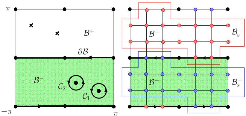
Figure 1: Left: The Brillouin zone, where shaded region denotes ${\cal B}^{-}$. The thick lines indicate the boundary of ${\cal B}^{-}$. The integration over ${\cal C}_{j}$ gives a winding number. Right: A lattice on the Brillouin zone. The sites in ${\cal B}_{\rm s}^{-}$, ${\cal B}_{\rm s}^{+}$, and ${\cal B}_{\rm s}^{0}$ are denoted by blue, red, and black circles, respectively. The shaded region denotes the plaquettes in ${\cal B}^{-}$.

In systems with breaking ${\cal T}$ symmetry like QH effect, such an obstruction gives in general a nontrivial Chern number. Contrary to this, in systems under consideration, the Chern number always vanishes due to ${\cal T}$ invariance. Even in this case, an obstruction occurs in the Brillouin zone as long as the zeros of the pfaffian exist. Since the zeros occur at the time reversed pairs of points $\pm k_{j}^{*}$, the vortices around these pairs are opposite and therefore cancel each other, giving vanishing Chern number. Nevertheless the sum of vorticities in half the Brillouin zone, e.g., in $\cal B^{-}$, just gives the number of zeros of $p(k)$ (mod 2). Imagine, for example, that two zeros exist in ${\cal B}^{-}$. Since they are generically first order zeros, the winding numbers are $\pm 1$. Then their sum is restricted to $\pm 2$ and 0, which can be denoted as “0 mod 2”. It thus turns out that the Fu-Kane formula (2) counts the vorticities in half the Brillouin zone. So far we have discussed in a specific gauge, but in any other gauge, $D$ changes by 2, provided that the gauge keeps ${\cal T}$ constraint. Therefore, $D$ is indeed a Z₂ topological invariant. It has also a topological stability against small perturbation as long as the many-body gap is finite. As we will show below, this expression for Z₂ invariant is convenient for numerical computations.

Define a lattice on the Brillouin zone,

$$k_{\ell}=\pi(j_{1}/N_{1},j_{2}/N_{2}),\quad j_{\mu}=-N_{\mu},\cdots,N_{\mu}.$$ (3)

The sites labeled by $k_{\ell}$ are divided into three sets, ${\cal B}_{\rm s}^{\pm}$ and ${\cal T}$ invariant sites ${\cal B}_{\rm s}^{0}$ denoted by red, blue and black circles in Fig. 1, respectively. Here, $\cal T$ invariant sites are specified by the property that ${\cal T}H(k_{\ell}){\cal T}^{-1}=H(k_{\ell})$. As a ${\cal T}$ constraint, we choose the states at $-k_{\ell}\in{\cal B}_{\rm s}^{+}$ as their Kramers doublets at $k_{\ell}\in{\cal B}_{\rm s}^{-}$. Suppose that at $k_{\ell}$ the spectrum is arranged as $\varepsilon_{n}(k_{\ell})\leq\varepsilon_{n+1}(k_{\ell})$. Then the states at $-k_{\ell}$ can be constrained as

$$|n(-k_{\ell})\rangle={\cal T}|n(k_{\ell})\rangle,\quad\mbox{for}\quad k_{\ell}\in{\cal B}_{\rm s}^{-}.$$ (4)

On the other hand, both of the Kramers doublets are included in ${\cal B}_{\rm s}^{0}$: The spectrum in this set can be arranged in general as $\varepsilon_{2n-1}(k)=\varepsilon_{2n}(k)\leq\varepsilon_{2n+1}(k)\cdots$. Therefore, we enforce the constraint

$$|2n(k_{\ell})\rangle={\cal T}|2n-1(k_{\ell})\rangle,\quad\mbox{for}\quad k_{\ell}\in{\cal B}_{\rm s}^{0}.$$ (5)

With these constrained states, we define a link variable

$$U_{\mu}(k_{\ell})={\cal N}_{\mu}^{-1}(k_{\ell})\det\psi^{\dagger}(k_{\ell})\psi(k_{\ell}+\hat{\mu}),$$ (6)

where ${\cal N}_{\mu}^{-1}(k_{\ell})=|\det\psi^{\dagger}(k_{\ell})\psi(k_{\ell}+\hat{\mu})|$, and associated field strength through a plaquette variable

$$F_{12}(k_{\ell}) =\ln U_{1}(k_{\ell})U_{2}(k_{\ell}+\hat{1})U_{1}^{-1}(k_{\ell}+\hat{2})U_{2}^{-1}(k_{\ell}),$$ (7)

where $F_{12}$ is defined within the branch $F_{12}/i\in(-\pi,\pi)$.

The sum of $F_{12}$ over ${\cal B}^{-}$ can be written as a similar formula to Eq. (2). To see this, it is convenient to define a gauge potential via $A_{\mu}(k_{\ell})=\ln U_{\mu}(k_{\ell})$ also in the branch $A_{\mu}(k_{\ell})/i\in(-\pi,\pi)$. Then the field strength can be rewritten as

$$F_{12}(k_{\ell}) =\Delta_{1}A_{2}(k_{\ell})-\Delta_{2}A_{1}(k_{\ell})+2\pi in_{12}(k_{\ell}),$$ (8)

where integral field $n_{12}(k_{\ell})$ has been introduced so as to match the branches of both sides Luescher99 ; FSW01 ; FHS05 . Thus, we reach

$$\sum_{k_{\ell}\in{\cal B}^{-}}F_{12}(k_{\ell})=\sum_{k_{\ell}\in\partial{\cal B}^{-}}A_{1}(k_{\ell})+2\pi i\sum_{k_{\ell}\in{\cal B}^{-}}n_{12}(k_{\ell}),$$ (9)

where the sums of $F_{12}$ and of $n_{12}$ are over the plaquettes in the shaded region denoted by ${\cal B}^{-}$ in Fig. 1. The sum of $A_{\mu}$ is over the links of the boundary of ${\cal B}^{-}$ specified by thick lines in Fig. 1. Therefore, a lattice version of $D$ is

$$D_{\rm L} \equiv\frac{1}{2\pi i}\left[\sum_{k_{\ell}\in\partial{\cal B}^{-}}A_{1}(k_{\ell})-\sum_{k_{\ell}\in{\cal B}^{-}}F_{12}(k_{\ell})\right]$$

$$=-\sum_{k_{\ell}\in{\cal B}^{-}}n_{12}(k_{\ell}).$$ (10)

This formula for the Z₂ invariants is one of the main results of this paper. Indeed this formula has the following desired properties. Firstly, it is strictly integral. Secondly, though the ground state multiplet can be mixed by Eq. (1), it is SU$(2M)$ invariant. Finally, it changes by 2 under the remaining U$(1)$ transformation, and hence, it is Z₂ invariant. The last property will be proved elsewhere, though it is not difficult.

In 3D, it has been shown that the phases of ${\cal T}$ invariant systems are classified by four independent Z₂ invariants MooBal06 ; Roy0607 ; FKM06 . To compute them, let us define six two-dimensional tori, according to Moore and Balents MooBal06 . For example, fix the third momentum to $k_{3}=0$ or $\pi$, then we have two tori spanned by $k_{1}$ and $k_{2}$ which we denote $Z_{0}$ and $Z_{\pi}$ torus, respectively. Applying the previous techniques, we can compute two Z₂ invariants $D_{\rm L}$ which are referred to as $z_{0}$ and $z_{\pi}$. In the same way, we have six invariants $x_{0}$, $x_{\pi}$, $y_{0}$, $y_{\pi}$, $z_{0}$, and $z_{\pi}$ living on six tori $X_{0}$, $X_{\pi}$, $Y_{0}$, $Y_{\pi}$, $Z_{0}$, and $Z_{\pi}$, respectively. There are two constraints, however: $x_{0}x_{\pi}=y_{0}y_{\pi}=z_{0}z_{\pi}$ (mod 2), and therefore, four invariants among six are independent MooBal06 . According to Fu et al. FKM06 , we choose them as $\nu_{0}=x_{0}x_{\pi}$, $\nu_{1}=x_{\pi}$, $\nu_{2}=y_{\pi}$, and $\nu_{3}=z_{\pi}$, and denote them as $\nu_{0};(\nu_{1}\nu_{2}\nu_{3})$. As is known in the QH effects, non-trivial structures of topological ordered states are hidden in the bulk and play physical roles near the boundaries as chracteristic edge states Hat93 . Based on the principle, by investigating the relationship between the Z₂ invariants and surface states, Fu et al. have clarified that there are basically three phases; simple band insulator, weak topological insulator (WTI) which is topological but weak against disorder, and more robust strong topological insulator (STI) FKM06 .

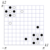
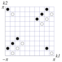
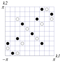
Figure 2: The $n$-field configurations for Bi (left two panels) and Sb (right two panels) computed by the gauge that the pfaffian is real positive. The first and third (second and fourth) show the configurations on the $Z_{0}$ ($Z_{\pi}$) torus. The white and black circles denote $n_{12}=1$ and $-1$, respectively, while the blank denotes 0. These read $z_{0}=2$ and $z_{\pi}=0$ for Bi, and $z_{0}=0$ and $z_{\pi}=1$ for Sb.

Recently, Murakami Mur06 has pointed out the possibility of QSH effect in Bi. Though Bi is a semimetal, the valence band and conduction band keep the direct gap throughout the Brillouin zone. Fu et al. have studied solvable tight-binding models with the diamond structure, and predicted that the valence band of Bi is characterized by the WTI phase specified 0;(111), based on the observation that the structure of Bi can be viewed as an adiabatically distorted cubic lattice toward the diamond lattice. However, since a realistic tight-binding model including $s$ and $p$ orbitals with nearest neighbor, second neighbor, and third neighbor hoppings has indeed complicated band structure, we calculate the Z₂ invariants directly for heavy group V elements.

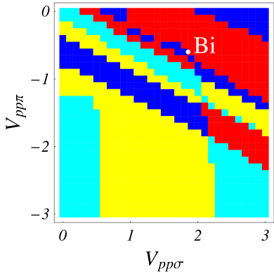
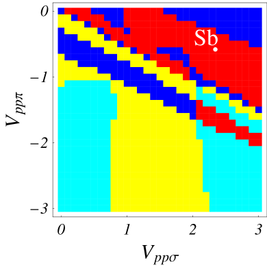
Figure 3: Phase diagrams of Bi (left) and Sb (right) as functions of $V_{pp\sigma}$ and $V_{pp\pi}$. Other parameters are the same as those in Ref. LiuAll95 . The colored regions denote different phases: red for 1;(111), yellow for 1;(000), lightblue for 0;(111), and blue for 0;(000). The white points indicate the position of the parameters for Bi and Sb in Ref. LiuAll95 .

In what follows, we investigate real materials by the tight-binding models in Ref. LiuAll95 . We first discuss the phase of Bi which is attracting much interest. We show in Fig. 2 examples of the $n$-field configuration computed for Bi. Though these calculations are for rather coarse $10\times 10$ lattice, we have checked that finer ones indeed reproduce the same Z₂ invariants and our formula is actually convergent even in this mesh size. For Bi, these figures tell that $z_{0}=z_{\pi}=0$ mod 2. The other Z₂ invariants are also 0 mod 2, and it turns out that the valence bands of Bi in 3D is specified by 0;(000) phase. This result is contradictory to the conjecture by Fu et al. mentioned-above. This suggests that along adiabatic distortion of the lattice, some topological changes should occur. Indeed, a slight change of the Slater-Koster parameters can lead to different phases. Among adjustable 14 parameters LiuAll95 , crucial ones may be $V_{pp\sigma}$ and $V_{pp\pi}$, nearest neighbor hopping parameters between $p$ orbitals. We show in Fig. 3 the phase diagram of Bi to discuss the stability of the phase. This diagram tells that Bi is located in a small island of 0;(000) phase embedded in 1;(111) phase. We also understand this feature from a small direct gap of Bi, 12 meV, at the $L$ point LiuAll95 . With varying the parameters, this gap soon closes and the phase of Bi changes from trivial phase into STI phase. We conclude that Bi in 3D dose not show the QSH effect, though it locates quite near the phase boundary with STI.

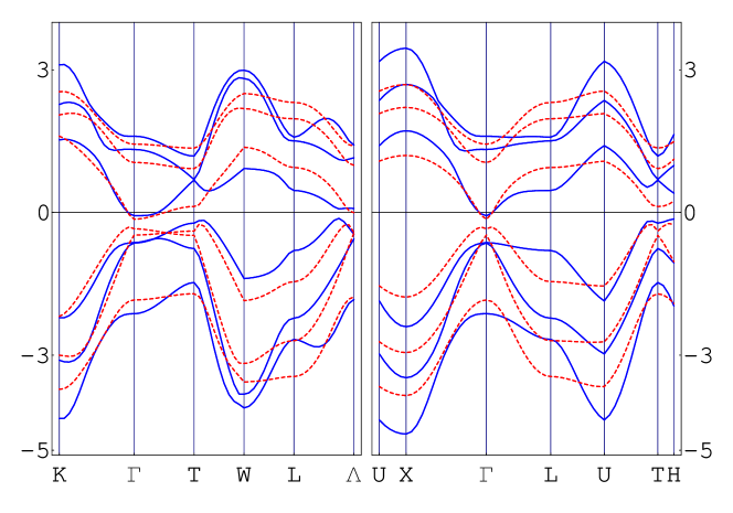
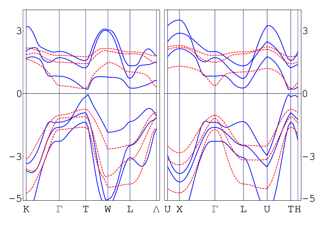
Figure 4: Band structure of Bi (upper) and Sb (lower). Bi: The blue lines are energies at $f=0.5$ and the red-dotted lines are at $f=0.1$. Sb: The blue lines at $f=0.7$ and the red-dotted lines at $f=0.1$. There are other bands around $-10$ eV associated mainly with $s$ orbitals which are omitted in these figures.

On the other hand, decreasing the thickness, a semimetal-semiconductor transition occurs, and Murakami has suggested that Bi thin film would be in QSH phase Mur06 . To study the quasi 2D systems, and also to clarify the discrepancy between our result and the conjecture by Fu et al., we next investigate the effects of dimensionality on the present model. We replace the Slater-Koster parameters $V^{\prime}_{\alpha}$ ($\alpha=ss\sigma,sp\pi,pp\sigma,pp\pi$) for second neighbor hopping in Ref. LiuAll95 by $fV^{\prime}_{\alpha}$ with a uniform factor $f$. This factor $f$ can effectively control the dimensionality into [111] direction, interpolating between Murakami’s model at $f=0$ and the 3D model at $f=1$.

We show in Fig. 4 the band structure of Bi with $f=0.5$ and $0.1$. At $f=1$ (See Ref. LiuAll95 ), the overlap energy (indirect gap) is $\Delta E=-12$ meV. With decreasing $f$, a semimetal-semiconductor transition occurs at $f\sim 0.99$. Fig. 4 confirms that Bi is indeed a semiconductor at $f=0.5$ and $0.1$ whose overlap energy is $\Delta E=56$ and $90$ meV, respectively.

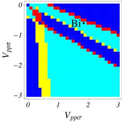
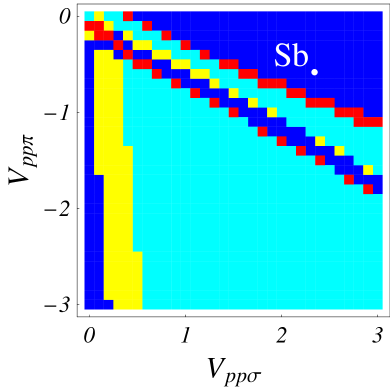
Figure 5: Phase diagrams of Bi (upper panel) and Sb (lower panel) for $f=0.1$ as functions of $V_{pp\sigma}$ and $V_{pp\pi}$.

Near $f=0.993$, the phase of Bi changes from 0;(000) into 1;(111). With further decreasing $f$ and enhancing the two-dimensionality, topological change occurs again near $f\sim 0.223$, and the system becomes 0;(111), as shown in Fig. 5. This is just the phase predicted by Fu et al. FKM06 . Therefore, we suggest that the adiabatic distortion of the diamond lattice leads to Bi thin film, and along the change of the dimensionality, the adiabatic distortion does not work, giving rise to gap-closing and resultant topological changes. We also conjecture that STI phase is very stable along the change of $f$, and could be observed by experiments.

Sb is also a semimetal with a larger gap at the $L$ point LiuAll95 . We show in Fig. 3 the phase diagram of Sb. It turns out that Sb belongs to the 1;(111) phase even in 3D. Its location is far from the phase boundary with 0;(000) and therefore, it is rather stable. We show in Fig. 4 the band structure of Sb. With decreasing $f$, a semimetal-semiconductor transition also occurs at $f\sim 0.89$. Along the change of $f$, topological change occurs once: Near $f\sim 0.54$, the phase changes from 1;(111) into 0;(000), and no 0;(111) phase is observed throughout. Therefore, the phase of Sb thin film is 0;(000), different from Bi. In Fig. 5, we show the phase diagram of Sb for $f=0.1$. However, it should be stressed that with appropriate thickness, $0.54\leq f\leq 0.89$, Sb is a semiconductor in STI phase and hence should show QSH effect.

Finally, we comment on the relationship between the method presented in this paper and the previous one in Ref. FukHat06 . While in the present calculation link variables are defined with respect to the momentum, the previous calculation has been implemented with respect to twist angles by imposing a spin-dependent twisted boundary condition. For systems with appropriate strength of spin-orbit coupling, the present computation is more efficient, but for systems with very small spin-orbit coupling as well as with inversion symmetry, the previous computation by the use of the twisted boundary condition gives more reliable results. In this sense, both methods are complementary to each other. Details will be published elsewhere.

We also mention that recently Fu and Kane FuKan06b have reached the similar conclusion of the phases of Bi and Sb by making the use of inversion symmetry of the system. We stress here that our method can apply to any systems, even without inversion symmetry.

This work was supported in part by Grant-in-Aid for Scientific Research (Grant No. 17540347, No. 18540365) from JSPS and on Priority Areas (Grant No.18043007) from MEXT. YH was also supported in part by the Sumitomo foundation.

References

- (1) C.L. Kane and E.J. Mele Phys. Rev. Lett. 95, 226801 (2005).
- (2) C.L. Kane and E.J. Mele Phys. Rev. Lett. 95, 146802 (2005).
- (3) B. A. Bernevig and S.-C. Zhang, cond-mat/0504147.
- (4) X.-L. Qi, Y.-S. Wu, and S.-C. Zhang, cond-mat/0505308.
- (5) L. Sheng, D.N. Sheng, C.S. Ting, and F.D.M. Haldane, cond-mat/0506589.
- (6) S. Murakami, N. Nagaosa, and S.-C. Zhang, Science 301, 1348 (2003); Phys. Rev. Lett. 93, 156804 (2004).
- (7) J. Sinova, D. Culcer, Q. Niu, N.A. Sinitsyn, T. Jungwirth, and A.H. MacDonald, Phys. Rev. Lett. 92, 126603 (2004).
- (8) Y.K. Kato, R.C. Myers, A.C. Gossard, and D.D. Awschalom, Science, 306, 1910 (2004).
- (9) J. Wunderlich, B. Kästner, J. Sinova, and T. Jungwirth, Phys. Rev. Lett. 94, 047204 (2005).
- (10) X.G. Wen, Phys. Rev. B 40, 7387 (1989).
- (11) Y. Hatsugai, J. Phys. Soc. Jpn. 73, 2604 (2004).
- (12) Y. Hatsugai, J. Phys. Soc. Jpn. 74, 1374 (2005).
- (13) D.J. Thouless, M. Kohmoto, M.P. Nightingale, and M. den Nijs, Phys. Rev. Lett. 49, 405 (1982).
- (14) M. Kohmoto, Ann. Phys. 160, 355 (1985).
- (15) Y. Yao, F. Ye, X.-L. Qi, S.-C. Ahang, and Z. Fang, cond-mat/0606350.
- (16) H. Min, J.E. Hill, N.A. Sinitsyn, B.R. Sahu, L. Kleinman, and A.H. MacDonald, cond-mat/0606504.
- (17) S. Murakami, cond-mat/0607001.
- (18) L. Fu, C.L. Kane, and E.J. Mele, cond-mat/0607699.
- (19) J.E. Moore and L. Balents, cond-mat/0607314.
- (20) R. Roy, cond-mat/0607531.
- (21) L. Fu and C.L. Kane, cond-mat/0606336.
- (22) T. Fukui, Y. Hatsugai, and H. Suzuki, J. Phys. Soc. Jpn. 74, 1674 (2005).
- (23) D.N. Sheng, Z.Y. Weng, L. Sheng, and F.D.M. Haldane, cond-mat/0603054.
- (24) T. Fukui and Y. Hatsugai, cond-mat/0607484.
- (25) R. Roy, cond-mat/0604211.
- (26) Y. Hatsugai, Phys. Rev. Lett. 71, 3697 (1993).
- (27) M. Lüscher, Nucl. Phys. B 549, 295 (1999).
- (28) T. Fujiwara, H. Suzuki, and K. Wu, Prog. Theor. Phys. 105, 789 (2001).
- (29) Y. Liu and R.R. Allen, Phys. Rev B 52, 1566 (1995).
- (30) L. Fu and C.L. Kane, cond-mat/0611341.