Determination of the spatial TDR-sensor characteristics in strong dispersive subsoil using 3D-FEM frequency domain simulations in combination with microwave dielectric spectroscopy

Abstract

The spatial sensor characteristics of a 6cm TDR flat band cable sensor section was simulated with finite element modelling (High Frequency Structure Simulator-HFSS) under certain conditions: (i) in direct contact to the surrounding material (air, water of different salinities, different synthetic and natural soils (sand-silt-clay mixtures)), (ii) with consideration of a defined gap of different size filled with air or water and (iii) the cable sensor pressed at a borehole-wall. The complex dielectric permittivity $\varepsilon^{\star}(\omega,\tau_{i})$ or complex electrical conductivity $\sigma^{\star}(\omega,\tau_{i})=i\omega\varepsilon^{\star}(\omega,\tau_{i})$ of the investigated saturated and unsaturated soils was examined in the frequency range 50MHz-20GHz at room temperature and atmospheric pressure with a HP8720D- network analyser. Three soil-specific relaxation processes are assumed to act in the investigated frequency-temperature-pressure range: one primary $\alpha$-process (main water relaxation) and two secondary ($\alpha^{\prime}$, $\beta$)-processes due to clay-water-ion interactions (bound water relaxation and the Maxwell-Wagner effect). The dielectric relaxation behaviour of every process is described with the use of a simple fractional relaxation model. 3D finite element simulation is performed with a $\lambda/3$ based adaptive mesh refinement at a solution frequency of 1MHz, 10MHz, 0.1GHz, 1GHz and 12.5GHz. The electromagnetic field distribution, S-parameter and step responses were examined. The simulation adequately reproduces the spatial and temporal electrical and magnetic field distribution. High-lossy soils cause depending on increasing gravimetric water content and bulk density an increase of TDR signal rise time as well as a strong absorption of multiple reflections. Air or water gap work as quasi wave-guide, i.e. the influence by surrounding medium is strongly reduced. Appropriate TDR-travel-time distortions can be quantified.

Keywords: lossy dielectrics, finite element modelling, HFSS, dielectric spectroscopy, fractional relaxation

1 Introduction

Soil science, geophysical prospecting, agriculture, hydrology, archeology and geotechnical engineering have benefited greatly from developments in radio and microwave technology. Electromagnetic techniques are used to estimate soil and rock physical characteristics such as water content, density and porosity ([47], [37], [27], [25]). Both invasive methods, such as time domain reflectometry ([49], [40], [15]) and cross borehole radar [10], and noninvasive methods, such as capacity methods ([46], [25], [27]) and ground penetrating radar ([24], [2], [42], [6], [13]) are used. Common to all these techniques is the fact that electromagnetic wave interaction depends on dielectric properties of rock or soil deposit through which it travels, which are influenced by chemical composition, mineralogy, structure, porosity, geological age and forming conditions. Besides, several additions like ubiquitous water have an effect on the dielectric properties.

In particular, knowledge of the spatial and temporal variability of water saturation in soils is important to obtain improved estimates of water flow (and its dissolved components) through the vadose zone. Due to its accuracy and potential for automated measurement, TDR has become one of the standard methods to measure spatial and temporal variability of water contents in laboratory soil cores and experimental field plots [15]. For this purpose, the object of numerous experimental and theoretical investigations is the development of general dielectric mixing models for a broad class of soil textures and structures ([49], [43], [50]). Mostly, these empirical, numerical or theoretical models base on the assumption of a constant dielectric permittivity of the soil as a function of volumetric water content in a narrow frequency range around 1GHz ([44], [48], [4], [9], [39]). However, the strong frequency dependence in the dielectric relaxation behaviour below 1GHz due to a certain amount of swelling clay minerals in nearly each real soil is considered only insufficiently ([30], [15], [32], [25]).

The type of multi-scale structure renders the analysis of dynamic data in clays rather complex. The problem has been addressed both by experimental and modelling techniques. Besides broadband dielectric spectroscopy on clay-water suspensions microscopic simulations of clays have been an active field of research since the late 1980s and began with simulations at ambient temperature and pressure, of clays with various cationic species. More recently, several studies appeared dealing with non-ambient conditions (increased temperatures and pressures), which are primarily linked to the issue of storage of radioactive waste or bore-hole stability [35]. Previous experimental and modelling results suggest that clay-water systems have multiple relaxation processes, such as interfacial polarizations around the clay particles and rotational relaxation of bound and free $H_{2}O$. Therefore, the dielectric behavior is expected to be complicated. Useful and precise dielectric information may only be obtained when each relaxation process is extracted from the complicated overall behavior based on the measurement of the complex dielectric permittivity over a broad frequency range and at high resolutions ([22], [21], [34], [33]).

In the present study, the the dielectric relaxation behaviour of the investigated saturated and unsaturated soils was examined in the frequency range 50MHz-20GHz. To parameterize the dielectric spectra three soil-specific relaxation processes are assumed to act as a function of water saturation and porosity in the investigated frequency-temperature-pressure range: one primary $\alpha$-process (main water relaxation) and two secondary ($\alpha^{\prime}$, $\beta$)-processes due to clay-water-ion interactions (bound water relaxation and the Maxwell-Wagner effect). The dielectric relaxation behaviour of every process is described with the use of a simple fractional relaxation model ([22], [21], [23], [19], [16]). The chosen approach enables a characterization of the dielectric relaxation behaviour with the separation in the observed relaxation processes in dependence of the porosity and the water content.

A simplification frequently utilized in TDR applications is the use of an idealized equivalent circuit for the sensor without consideration of losses due to the skin-effect or radiation from the sensor as well as the assumption of a homogeneous sensitivity distribution along the sensor ([15], [20], [45], [28]). In addition, a frequently arising problem in various applications is the direct contact between sensor, e.g. a flexible band cable, and surrounding medium. An air or water gap between sensor and soil leads to dramatic under or overestimation of water content. A suitable tool for an examination of this specific problems offers three-dimensional numeric finite element simulation ([28]). For these reasons, in this study the spatial sensor characteristics of a 6cm TDR flat band cable sensor section was simulated with electromagnetic finite element modelling (Ansoft-HFSS^TM , High Frequency Structure Simulator). In order to carry out the finite element calculations as realistically as possible, the measured frequency-dependent dielectric permittivity was considered. Moreover, the simulations were performed under certain conditions: (i) in direct contact to surrounding material, (ii) with consideration of a defined gap of variable size filled with air or water and (iii) cable sensor pressed at a borehole-wall.

2 Theoretical Background

Time domain reflectometry measures the propagation velocity of a broadband step voltage pulse (typical values: rise time $t_{r}\approx 70ps$, sampling increment $\Delta t\approx 20ps$) with a bandwidth of around 20kHz to  25GHz (Nyquist-frequency: $f_{max}=0.5/\Delta t$). But due to the limitations of used connectors, type of the TDR device, coaxial cable type and length the effective bandwidth is reduced distinctly [31]. Under atmospheric conditions the velocity of this signal is a function of the frequency $\omega=2\pi f$ and temperature $T$ dependent effective relative complex permittivity $\varepsilon_{{\mbox{eff}}}^{\star}(\omega,T)=\varepsilon_{\mbox{eff}}^{\prime}(\omega,T)-j\varepsilon_{\mbox{eff}}^{\prime\prime}(\omega,T)$ of the material through which it travels. The overall losses $\varepsilon_{\mbox{eff}}^{\prime\prime}(\omega,T)=\varepsilon_{d}^{\prime\prime}(\omega,T)+\frac{\sigma_{DC}(T)}{\omega\varepsilon_{0}}$ of the material which have to be considered result from the dielectric losses $\varepsilon_{d}^{\prime\prime}(\omega,T)$ and the conductive losses $\frac{\sigma_{DC}(T)}{\omega\varepsilon_{0}}$ due to a direct current electrical conductivity $\sigma_{DC}(T)$. Here, $\varepsilon_{0}$ is the permittivity of free space and $j^{2}=-1$ is the imaginary unit. It is often convenient to consider the analogy of propagation phase velocity and attenuation of an electromagnetic plane wave (see [49], [6], [15], [41]):

$$v_{P}(\omega,T)=c\sqrt{2}\left({\sqrt{\sqrt{\varepsilon^{\prime}_{{\mbox{eff}}}(\omega,T)^{2}+\varepsilon^{\prime\prime}_{{\mbox{eff}}}(\omega,T)^{2}}+\varepsilon^{\prime}_{{\mbox{eff}}}(\omega,T)}}\right)^{-1}$$ (1)

$$\beta(\omega,T)=\omega\sqrt{\sqrt{\varepsilon^{\prime}_{{\mbox{eff}}}(\omega,T)^{2}+\varepsilon^{\prime\prime}_{\mbox{eff}}(\omega,T)^{2}}-\varepsilon^{\prime}_{\mbox{eff}}(\omega,T)}\cdot\left({c\sqrt{2}}\right)^{-1}$$ (2)

where $c=\sqrt{\varepsilon_{0}\mu_{0}}^{-1}$ is the velocity of light and $\mu_{0}$ the magnetic permeability of vacuum. Hence, any modulation of an electromagnetic wave in a real medium will propagate at a group velocity according to the Rayleigh equation ([11], [12]):

$$v_{g}=\frac{{d\omega}}{{dk}}=v_{P}\left[{1-\frac{f}{{v_{P}}}\frac{{dv_{P}}}{{df}}}\right]^{-1}$$ (3)

herein, $k$ denotes the wave number. The flat band cable of length $l$ consists of three strip conductors embedded in a polyethylene band (see [20], [27] for details). The effective group or phase velocity of the signal $v^{\prime}_{P}$ in a perfect dielectric (pure real dielectric constant $\varepsilon_{r}=\varepsilon_{\mbox{eff}}^{\star}=\hbox{const}$ without dispersion and conducting losses) surrounding the cable sensor is in principle only a crude approximation of the real material properties especially at frequencies $f<1GHz$ and $f>10GHz$ (c.f. Fig. 1)

$$v^{\prime}_{P}=v_{g}=\frac{{2l}}{t}=\frac{c}{{\sqrt{\varepsilon_{r}}}}$$ (4)

where $t$ is two way travel time. Considering anomalous dispersion equation (4) is referred to as a high frequency approximation of phase velocity (Fig. 1). In contrast the high frequency attenuation approximation $\beta_{h}\left(\omega,T\right)$ for real soils frequently used in ground penetrating radar applications works considerably well (c.f. [6], Fig. 1)

$$\beta_{h}\left(\omega,T\right)=\frac{{\omega\varepsilon_{0}\varepsilon^{\prime\prime}_{{\mbox{eff}}}(\omega,T)}}{{\sqrt{\varepsilon^{\prime}_{{\mbox{eff}}}(\omega,T)}}}\frac{Z_{0}}{2}$$ (5)

• 
  

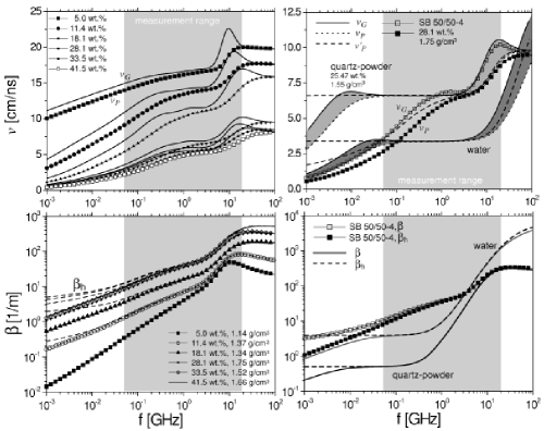
Figure 1: (top) Phase velocity $v_{P}$, high frequency approximation $v_{p}^{\prime}$, corresponding group velocity $v_{g}$ as well as (bottom) attenuation $\beta$ and corresponding high frequency approximation $\beta_{h}$ of (left) a sand-bentonite mixture (SB 50/50 1-6) with different gravimetric water content $\theta_{g}$ and bulk density $\varrho$ (see section 3, Tab. 2, Fig. 5). (right) Comparison of natural water with $\sigma_{DC}=0.18S/m$, a mikrosil quartz powder and SB 50/50-4 (see Tab. 1 and 2 below). The calculations were carried out under utilization of the measured dielectric permittivity.

with impedance $Z_{0}=c\mu_{0}$ of vacuum. We now consider the soil as a four-phase medium composed of: air, quartz grain, water and clay. In the particular case of spatial TDR the surrounding medium in the direction oft the band cable is described by a relative effective permittivity $\varepsilon^{\star}_{\mbox{eff}}(x,\omega,T,p)$. It depends on position $x$, angular frequency $\omega$ and contribution due to several relaxation processes via relaxation time $\tau(T,p)$ on absolute temperature $T$ and pressure $p$ ([22], [30])

$$\tau_{i}(T,p)=\kappa_{i}\frac{h}{{k_{B}T}}\exp\left({\frac{{E_{a,i}(T,p)}}{{RT}}}\right)$$ (6)

Herein, $h$ denotes the Planck-constant, $k_{B}$-Boltzmann constant, $\kappa_{i}\approx 1$ the transmission coeffitient, $R$ gas constant and $E_{a,i}(T,p)=\Delta G_{i}(T,p)+T\Delta S_{i}(T,p)$ activation energy with free enthalpy $\Delta G_{i}(T,p)$ and activation entropy $\Delta S_{i}(T,p)$ of the $i$-th process ([22], [21]). Dielectric loss spectra of saturated and unsaturated soils very often show a marked deviation from simple Debye-behaviour ([17], [19], [22], [25]). Based on the theory of fractional time evolutions Hilfer [16] derived a Jonscher type function [23] for the complex frequency dependent dielectric permittivity of amorphous and glassy materials

$$\tilde{\varepsilon}_{{\mbox{eff}},i}(\omega,\tau_{i})-\varepsilon_{\infty}=\frac{{\Delta\varepsilon_{i}(T)}}{{\left({j\omega\tau_{i}}\right)^{\alpha_{i}}+\left({j\omega\tau_{i}}\right)^{\beta_{i}}}}$$ (7)

with high frequency limit of permittivity $\varepsilon_{\infty}$, relaxation strength $\Delta\varepsilon_{i}(T)$ as a function of temperature, angular frequency $\omega$ and stretching exponents $0\leq\alpha_{i},\beta_{i}$ similar to the familiar empirical Havriliak and Negami [14], Cole-Cole [3], Cole-Davidson [5] or Kohlrausch-Williams-Watts ([26], [51]) dispersion and absorption functions. For the particular case $\alpha_{i}=0$ and $\beta_{i}=1$ (7) transforms to the Debye model.

3 Material and Experiments

• 

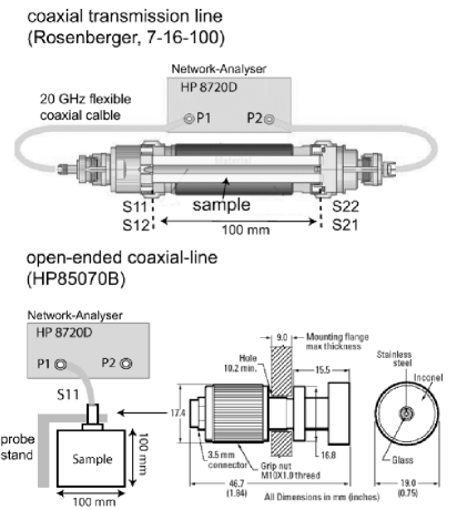
Figure 2: Schematic diagram of the experimental set-up for measuring the dielectric permittivity: (top) longitudinal section of the coaxial transmission line with an outer diameter of the inner conductor $d_{i}=7mm$, an inner diameter of the outer conductor $d_{o}=16mm$ and a length $l=100mm$, (bottom) open-ended coaxial-line (HP85070B).

The complex effective dielectric permittivity $\varepsilon_{\mbox{eff}}^{\star}$ of saturated and unsaturated soils was examined in the frequency range 50MHz-20GHz at room temperature and atmospheric pressure with a HP8720D- network analyser. This was performed using a combination of open-ended coaxial-line (HP85070B) and coaxial transmission line technique (sample holder (7x16x100)mm³) (Fig. 2). The synthetic soil samples were incrementally wetted from air dry up to saturation with natural water and equilibrated 12h. From the prepared sample a subsample was taken with a retaining ring (hight 100 mm, inner diameter 100 mm). The retaining ring was used as the sample holder for the HP85070B probe. Care was taken to pack the soil in the transmission line to a homogeneous bulk density $\varrho$ and to a constant volume. After each dielectric measurement bulk density $\varrho$ as well as gravimetric water content $\theta_{g}$ were determined. The measured complex S-parameter values $S_{ij}$ were used to calculate complex dielectric permittivity with a commercial software (HP 85070/71C Materials Measurement Software) after calibration with open, short, and load standards.

Different natural and synthetic soils were investigated. Here, we present our results for synthetic soil SB50/50. It is a mixture of 50wt.% sand (grain size $<$2mm) and 50 wt.% bentonite (Calcigel: 71wt.% Ca- dioctahedral smectite, 9wt.% illite/dioctahedral mica, 1wt.%kaoline, 1wt.% chlorite, 9wt.% quartz, 5wt.% feldspar, 2wt.% calcite, 2wt.% dolomite).

Ca- dioctahedral smectites are clay minerals, i.e. they consist of individual crystallites the majority of which are $<$2$\mu$m in largest dimension. The crystal structure of clays has been established from X-ray diffraction studies for almost all types of common clays. Smectite crystallites themselves are three-layer clay minerals. Individual clay layers consist of fused sheets of octahedra of Al³⁺ or Mg²⁺ oxides and tetrahedra of Si⁴⁺ oxides. Substitution of Al³⁺, Mg²⁺ or Si⁴⁺ with lower valence ions results in an overall negative charge on the layers, which is then compensated by cationic species (counterions, in the current case $Ca^{2+}$) between clay layers (interlayers) ([29], Fig. 3).

• 

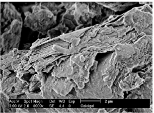
Figure 3: SEM-EDX micrograph of the investigated bentonite Calcigel, Philips XL30 ESEM-FEG.

Table 1: Physical properties of the investigated bentonite (^♭[8]) in comparison to the commercial Mikrosil quartz powder (type 350, median grain size 11$\mu m$).

	Ca-Bentonite	Mikrosil
Dry density $\varrho_{d}$	1.33 g/cm3	0.69 g/cm3
Specific surface area	493 m2/g(♭)	0.38 m2/g
Density	2.847 g/cm3	2.65 g/cm3
Cation exchange capacity	62.0 meq/100g(♭)

Under increasing relative humidity the compensating ions become hydrated and the spacing between individual layers increases. While the detailed swelling characteristics of a smectite (interlayer spacing as a function of relative humidity) depends crucially on the charge of the clay layers (magnitude and localisation) and the nature of the compensating ion, in general, it occurs in three stages. Swelling begins in a step-wise manner (discrete layers of water formed in the interlayer, states referred to as monolayer/monohydrated, bilayer/ bihydrated, etc.), becomes continuous thereafter and in the extreme a colloidal suspension of clay particles ($<$10 aligned layers) is formed. Beyond the microscopic scale, aggregates of aligned clay layers form particles of the order of 10 nm - 1000 nm in size, with porosities on the meso- (8 nm - 60 nm) and macroscale ($>$60 nm) ([35] and citations in it). In Tab. 1 the physical and chemical properties of the used bentonite calcigel are summarized.

• 

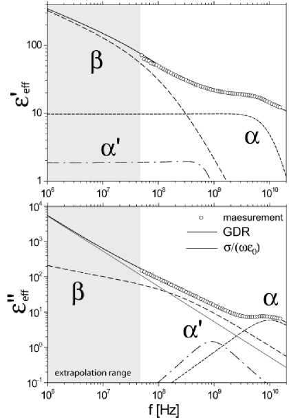
Figure 4: Complex relative dielectric permittivity $\varepsilon^{\star}_{\mbox{eff}}=\varepsilon^{\prime}_{\mbox{eff}}-j\varepsilon^{\prime\prime}_{\mbox{eff}}$ as a function of frequency of sand-bentonite-mixture SB50/50-4 with GDR-fit under consideration of three relaxation processes: one primary $\alpha$-process (main water relaxation) and two secondary ($\alpha^{\prime},\beta$)-processes due to clay-water-ion interactions (bound water relaxation and the Maxwell-Wagner effect). In this way it was possible to separate the singe relaxation processes and to extrapolate the dielectric permittivity to 1MHz.

Three relaxation processes are assumed to act in the investigated frequency-temperature-pressure range: one primary $\alpha$-process (main water relaxation) and two secondary ($\alpha^{\prime},\beta$)-processes due to clay-water-ion interactions (bound water relaxation and the Maxwell-Wagner effect, see Fig. 4). The effective permittivity of a multiphase soil-mixture $\varepsilon^{\star}_{\mbox{eff}}$ can be determined by the complex relative permittivity of water $\varepsilon^{\star}_{w}$, bound water $\varepsilon^{\star}_{bw}$, the contribution due to clay-water-ion interaction $\varepsilon^{\star}_{clay}$ as well as the real and constant permittivity of quartz grain $\varepsilon_{sand}$ and air ([47], [37], [44], [48], [22], [21], [4]). The dielectric relaxation behaviour of each process is described by a fractional relaxation model according to (7) considering relaxation time distributions $H(\tau)$. This allows the complete spectrum to fit as a function of water content $\theta_{g}$ and bulk density $\varrho$ at constant temperature and pressure with the use of a generalized dielectric response (GDR, Fig. 4 and 5):

$$\varepsilon_{\mbox{eff}}^{\star}(\omega)-\varepsilon_{\infty}=\sum\limits_{i=1}^{3}{\frac{{\Delta\varepsilon_{i}}}{{\left({j\omega\tau_{i}}\right)^{\alpha_{i}}+\left({j\omega\tau_{i}}\right)^{\beta_{i}}}}}-j\frac{{\sigma_{DC}}}{{\omega\varepsilon_{0}}}$$ (8)

• 

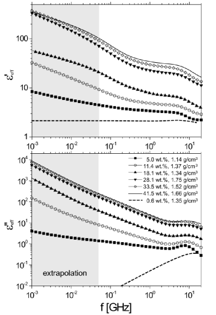
Figure 5: Dispersion and absorption curve of sand-bentonite-mixture (SB50/50) for seven gravimetric water contents $\theta_{g}$ and bulk densities $\varrho$.

Table 2: Parameters of the three relaxation processes from GDR-fitting ($i=[\alpha,\alpha^{\prime},\beta]$); gravimetric water content $w$, bulk density $\varrho$, porosity $n$, water saturation $S_{w}$ and volumetric water content $\theta=S_{w}n$ of SB-50/50.

• 	50-0	50-1	50-2	50-3	50-4	50-5	50-6	Mikrosil
  $w$ $[\%]$	0.6	5	11.4	18.1	28.1	33.5	41.5	25.47
  $\varrho$ $[g/cm^{3}]$	1.35	1.14	1.37	1.34	1.75	1.52	1.66	1.55
  $n$	0.5	0.6	0.55	0.59	0.53	0.62	0.64	0.56
  $S_{w}$	0.02	0.09	0.25	0.34	0.66	0.54	0.63	0.71
  $\theta$ $[\%]$	0.81	5.42	13.84	19.86	35.36	33.86	40.3	39.48
  $\varepsilon_{\infty}$	1.03	1.15	1.23	2.07	3.38	3.77	6.69	1.26
  $\Delta\varepsilon_{\alpha}$	0.86	0.05	0.01	0.13	5.44	3.67	19.57	16.73
  $\tau_{\alpha}$ $[ps]$	4.99	9.18	8.44	7.43	6.06	8.74	9.8	9.25
  1-$\beta_{\alpha}$	0.004	0.004	0.07	0.025	0.075	0.091	0.095	0.002
  $\alpha_{\alpha}$ (fixed)	0	0	0	0	0	0	0	0
  $\Delta\varepsilon_{\alpha^{\prime}}$	0.25	2.16	3.18	5.06	10.31	19.7	5.77	2.09
  $\tau_{\alpha^{\prime}}$ $[ps]$	5.37	9.64	9.34	9.63	9.93	9.7	9.32	0.27
  1-$\beta_{\alpha^{\prime}}$	0.004	0.081	0.081	0.075	0.003	0.082	0.034	0.048
  $\alpha_{\alpha^{\prime}}$ (fixed)	0	0	0	0	0	0	0	0
  $\Delta\varepsilon_{\beta}$	0.05	1.57	4.9	11.06	43.35	62.17	74.99	0.87
  $\tau_{\beta}$ $[ns]$	98.46	0.5	0.6	0.51	0.52	0.65	0.83	22.6
  1-$\beta_{\beta}$	0.65	0.99	0.56	0.69	0.66	0.68	0.74	0.92
  $\alpha_{\beta}$ (fixed)	1	1	1	1	1	1	1	1
  $\sigma_{DC}$ $[mS/cm]$	6.68E-5	0.03	0.05	0.75	3.37	4.62	5.31	0.12

A Shuffled Complex Evolution Metropolis (SCEM-UA) algorithm is used to find best GDR fitting parameters [15], Tab. 2). This algorithm is an adaptive evolutionary Monte Carlo Markov Chain method inspired by the SCE-UA global optimization algorithm of [7] and combines the strengths of the Metropolis algorithm [36], controlled random search [38], competitive evolution [18], and complex shuffling [7] to obtain an efficient estimate of the most optimal parameter set, and its underlying posterior distribution, within a single optimization run. The resulting relative error of each parameter is less than 3%.

• 

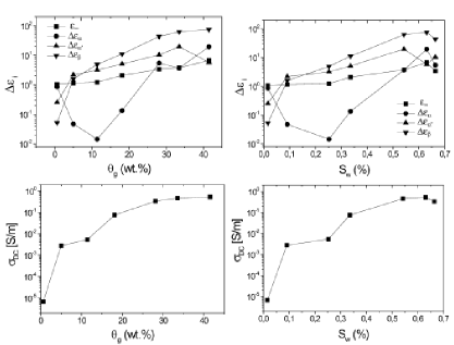
Figure 6: (top) Relaxation strength $\Delta\varepsilon_{i}$ of the i-th process in comparison to the relative high frequency permittivity $\varepsilon_{\infty}$ as a function (left) of gravimetric water content and (right) water saturation $S_{w}$. (bottom) Apparent direct current electrical conductivity $\sigma_{DC}$.

The relaxation parameters obtained from GDR-fit are presented in Fig. 6. Relaxation strength $\Delta\varepsilon_{i}$ of each process and relative high frequency permittivity $\varepsilon_{\infty}$ depend on moisture content. Above a gravimetric water content of $\approx 30wt.\%$ the $\alpha^{\prime}$-process decrease and the $\alpha$-process strongly increase. This suggest an increase of the primary $\alpha$-relaxation at the expense of the bound water process $\alpha^{\prime}$. In contrast at the highest saturation level of 0.66 at a porosity of 0.53 primary $\alpha$ and low frequency $\beta$-process decrease. Relaxation time $\tau_{i}$ and distribution parameter $\beta_{i}$ are nearly constant. An exception represents sample 50-0 which shows clear deviation from the general trend but because of the very low gravimetric water content of 0.6 wt%. Without swelling an increasing saturation reduces the gas-filled pore space, while the effective pore space available for the fluid becomes larger. This leads to the simple calibration models mentioned in the introduction to determine the volumetric water content with dielectric measurements. Due to the swelling of the clay minerals in the process of the hydration the distribution of immobile and effective pore space cannot be considered as constant. A circumstance which complicate a careful realization of accurate measurements is the fact that a multitude of variables of the measurement conditions and the sample preparation essential determine the intensity of the swelling and the resulting change of the pore structure ([1]).

The results show the potential of the chosen approach but a detailed explanation of this complex behavior is beyond the scope of this paper. In general, there is a need of further systematic investigations by broadband dielectric spectroscopy of saturated and unsaturated soils under consideration of the swelling process and with an utilisation of microscopic modelling.

• 

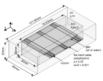
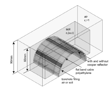
Figure 7: Model geometry of (top) flat band cable surrounded by saturated and unsaturated soil with a gap filled with air or water and (bottom) cable sensor pressed at a borehole-wall with air or soil as borehole filling.

4 HFSS-Simulations

The transfer or scattering function $S_{ij}(\omega)$ of the flat band cable section (Fig. 7) was simulated by finite element modelling (commercial software from Ansoft: High Frequency Structure Simulator-HFSS) under certain conditions: (i) in direct contact to the surrounding material (air, water of various salinities, different synthetic and natural soils (sand-silt-clay mixtures)), (ii) with consideration of a defined gap of various size (total high 2 mm, 3 mm, 5 mm, 7 mm or 10 mm) filled with air or distilled water and (iii) cable sensor pressed at a borehole-wall.

In HFSS tangential element basis function interpolates field values from both nodal values at vertices and on edges. Surfaces of the structure (air-box) in the y-z an x-y plane are radiation boundaries and the second-order radiation boundary condition is used

$$\nabla\times\vec{E}_{t}=jk_{0}\vec{E}_{t}-\frac{j}{k_{0}}\nabla_{t}\times(\nabla_{t}\times\vec{E}_{t})+\frac{j}{k_{0}}\nabla_{t}(\nabla_{t}\bullet\vec{E}_{t})$$ (9)

where $\vec{E}_{t}$ is the component of the E-field that is tangential to the surface and $k_{0}$ is the free space phase constant. The second-order radiation boundary condition is an approximation of free space. The accuracy of the approximation depends on the distance between the boundary and the object from which the radiation emanates. For this reason a sensitivity analysis was carried out for a total height of the structure between 20 mm and 50 mm in dependence of the material properties. The influence of the boundary layer for the simulation into air can be neglected for a distance from the cable sensor greater than 12 mm so a minimum height of 25 mm is used.

Surfaces in the x-z plane are wave ports. HFSS assumes that each wave port is connected to a semi-infinitely long waveguide that has the same cross-section and material properties as the port. When solving for the S-parameters, HFSS assumes that the structure is excited by the natural field patterns (modes) associated with these cross-sections. The 2D field solutions generated for each wave port serve as boundary conditions at those ports for the 3D problem. The final field solution computed must match the 2D field pattern at each port.

• 

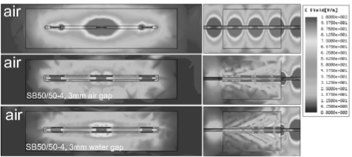
Figure 8: Electric field distribution $@12.5GHz$ for the investigated flat band cable surrounded by air, sand-bentonite-mixture (SB 50/50-4) with $\theta_{g}=$28.14wt.% and $\rho=1.79g/cm^{3}$ as well as a defined 3mm air or water gap. (left) Cross section, (right) longitudinal section of middle conductor.

The simulation is performed with a $\lambda/3$ based adaptive mesh refinement at solution frequency of 1 MHz, 10 MHz, 0.1 GHz, 1 GHz and 12.5 GHz. Broadband complex S-Parameter are calculated with an interpolating sweep in frequency range 1 MHz - 12.5 GHz with extrapolation to DC. The electromagnetic field distribution, S-parameter and step response (200 ps rise time) of the structure were computed in reflection and transmission mode.

• 

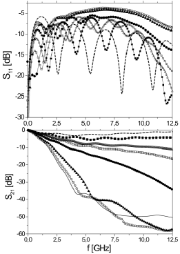
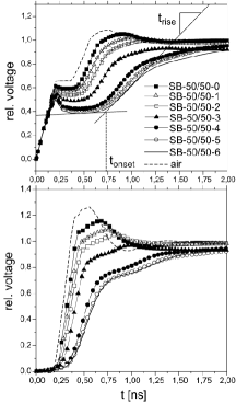
Figure 9: (left) Input return loss magnitude or reflection coefficient $S_{11}$ and forward transmission or transmission coefficient $S_{21}$ as well as (right) TDR-waveform in reflection and transmission mode for simulated flat band cable structure, surrounded by air and sand bentonite mixture of various water contents and bulk densities (see Tab. 2).

5 Discussion

The simulation adequately reproduces the spatial and temporal electrical and magnetic field distribution in comparison with 2D-FE investigations of [20] (Fig. 8). Fig. 9 represents reflection and transmission factor as well as the corresponding TDR waveform for the sand-bentonite mixture at various water contents and bulk densities in reflection and transmission mode. As a reference material the simulation results for the cable sensor surrounded by air are included. As expected, the appropriate resonances in the reflection coefficient $S_{11}$ shift with rising water content to deeper frequencies and the attenuation increases. In time domain onset travel-time as well as rise time of the TDR signals are analyzed. As is clearly recognizable in both reflection and transmission mode, onset time increase and rise time decrease with rising water content.

Qualitatively the numerical calculation shows that sensitivity characteristic of the cable sensor changes along the sensor in dependents of the dielectric relaxation behavior of the surrounding material (Fig. 8). The investigated high-lossy sand-bentonite mixture cause in dependence of increasing gravimetric water content $\theta_{g}$ and bulk density $\varrho$ an increase of TDR signal rise time as well as a strong absorption of multiple reflections. This leads to a frequency dependent decrease of spatial resolution and penetration depth (sensitivity region around the sensor) along the flat band cable and fixed maximal length of the moisture-sensor available for application.

Coupling problems caused by air or water gaps lead to dramatic travel time distortion even for very small gaps (Fig. 10). The air filled gap with a thickness of 0.25mm on both sides of the cable sensor already leads to the drastic underestimation of water content of 36%. In contrast a drastic overestimation occurs in the case of a water filled gap for the same gap size. Further increasing gap size leads to a maximum in the characteristic (anomal behavior) at a gap thicknesses of approximately 2.7 mm, whereby up to the complete filling of the structure with water the effective dielectric constant decrease and the rise time increase. An explanation of this effect and the consequences linked with it are however still pending and require further numerical and experimental investigations. Moreover, with HFSS it is not possible to consider an exchange of material between air or water-filled gap and surrounding medium.

As a consequence the gap work as quasi waveguide, i.e. the influence of the surrounding medium is strongly reduced but changes in dielectric properties along the cable sensor are reproduced.

• 

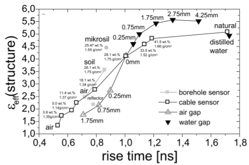
Figure 10: Real effective relative permittivity $\varepsilon_{\mbox{eff}}=2l/t_{\mbox{onset}}$ according to equation (4) plotted against TDR rise time $t_{\hbox{rise}}$ (in reflection mode) for all sensor configurations and investigated cases.

6 Conclusion

In this study, the spatial sensor characteristics of a 6cm TDR flat band cable section is simulated with finite element modelling in combination with dielectric spectroscopy.

For this purpose the dielectric relaxation behaviour of saturated and unsaturated soils is examined in the frequency range 50MHz-20GHz. The dielectric relaxation behaviour is described with the use of a generalized fractional relaxation model. With this approach the frequency depended dielectric permittivity is determined based on a parametrization of each relaxation processes as a function of water content and porosity. This enables a development of improved calibration strategies. However, there is a need of further systematic investigations by broadband dielectric spectroscopy of saturated and unsaturated soils under consideration of the swelling process and with an utilisation of microscopic modelling.

The three-dimensional numeric finite element simulation in HFSS provide an informative basis of the sensor characteristics under consideration of the frequency dependence of the measured complex dielectric permittivity. It is shown, that an air or water gap between sensor and soil leads to dramatic under or overestimation of water content already for a gap thickness of 0.25 mm upper and below the cable sensor. Therefore, the application of the flat cable as a moisture sensor requires an accurate installation technique of cable-like elements (especially for long sensors). Moreover, the spacial sensitivity characteristics of the cable sensor changes along the sensor in dependents of the dielectric relaxation behavior of the surrounding material. For this reason, the precise determination of soil moisture profiles requires an improved TDR-waveform analysis strategy under consideration of the change of the sensitive area along the cable sensor.

A disadvantage of the used FEM with HFSS is the lack of consideration an exchange of material between air or water-filled gap and surrounding medium. In addition, to achieve sufficient accuracy the numerical simulations with HFSS requires a high degree of computational cost in terms of computational time and memory. Further, theoretical, numerical, and experimental investigations in conjunction with reconstruction algorithms have to point out to what extent the accuracy of water content and porosity profiles can be determined in strong dispersive, high lossy materials.

References

References

- [1] S. S. Agus and T. Schanz. Comparison of Four Methods for Measuring Total Suction. Vadose Zone J, 4(4):1087–1095, 2005.
- [2] A. P. Annan, W. M. Waller, D. W. Strangway, J. R. Rossiter, J. D. Redman, and R. D. Watts. The electromagnetic response of a low-loss, 2-layer, dielectric earth for horizontal electric dipole excitation. Geophysics, 40(2):285–298, 1975.
- [3] K.S. Cole and R.H. Cole. Dispersion and Absorption in Dielectrics. Journal of Chemical Physics, 9(4/41):341–351, 1941.
- [4] Ph. Cosenza and A. Tabbagh. Electromagnetic determination of clay water content: role of the microporosity. Applied Clay Science, 26(1-4):21–36, 2004.
- [5] D. Davidson and R. Cole. Dielectric relaxation in glycerol, propylene glycol, and n-propanol. Journal of Chemical Physics, 19:1484–1490, 1951.
- [6] J.L. Davis and A.P. Annan. Ground-penetrating radar for high-resolution mapping of soil and rock stratigraphy. Geophysical Prospecting, 37:531–551, 1989.
- [7] Q. Duan, S. Sorooshian, and V. Gupta. Effective and efficient global optimization for conceptual rainfall-runoff models. Water Resources Research, 28(4):1015–1031, 1992.
- [8] I. Engelhardt, S. Finsterle, and C. Hofstee. Experimental and Numerical Investigation of Flow Phenomena in Nonisothermal, Variably Saturated Bentonite-Crushed Rock Mixtures. Vadose Zone J, 2(2):239–246, 2003.
- [9] S. R. Evett and G. W. Parkin. Advances in Soil Water Content Sensing: The Continuing Maturation of Technology and Theory. Vadose Zone J, 4(4):986–991, 2005.
- [10] T. Fechner, F. Börner, T. Richter, U. Yaramancy, and B. Weihnacht. Near Surface Geophysics, 23:150–159, 2004.
- [11] B. Forkmann and H. Petzold. Prinzip und Anwendung des Gesteinsradars zur Erkundung des Nahbereiches. VEB Deutscher Verlag für Grundstoffindustrie Leipzig, 1989.
- [12] W. Greiner. Classical Electrodynamics. Springer, 1998.
- [13] S. Hanafy and S. A. al Hagrey. Ground-penetrating radar tomography for soil-moisture heterogeneity. Geophysics, 71(1):K9–K18, 2006.
- [14] S. Havriliak and S. Negami. A complex plane representation of dielectric and mechanical relaxation processes in some polymers. Polymer, 8(4):161–210, 1967.
- [15] T. J. Heimovaara, J.A. Huisman, J. A. Vrugt, and W. Bouten. Obtaining the Spatial Distribution of Water Content along a TDR Probe Using the SCEM-UA Bayesian Inverse Modeling Scheme. Vadose Zone J, 3:1128–1145, 2004.
- [16] R. Hilfer. H-function representations for stretched exponential relaxation and non-debye susceptibilities in glassy systems. Physical Review E (Statistical, Nonlinear, and Soft Matter Physics), 65(6):061510, 2002.
- [17] P. Hoekstra and A. Delaney. Dielectric properties of soils at UHF and microwave frequencies. Journal of Geophysical Research, 79(11):1699–1708, 1974.
- [18] J. H. Holland. Adaptation in natural and artificial systems. The University of Michigan Press, 1975.
- [19] F. Hollender and S. Tillard. Modeling ground-penetrating radar wave propagation and reflection with the jonscher parameterization. Geophysics, 63(6):1933–1942, 1998.
- [20] C. Hübner, S. Schlaeger, R. Becker, A. Scheuermann, A. Brandelik, W. Sch del, and R. Schuhmann. Electromagnetic Aquametry, chapter Advanced measurement methods in time domain reflectometry for soil moisture determination., pages 317–347. Springer, 2005.
- [21] T. Ishida, M. Kawase, K. Yagi, J. Yamakawa, and K. Fukada. Effects of the counterion on dielectric spectroscopy of a montmorillonite suspension over the frequency range Hz. Journal of Colloid and Interface Science, 268(1):121–126, 2003.
- [22] Tomoyuki Ishida, Tomoyuki Makino, and Changjun Wang. Dielectric-relaxation spectroscopy of kaolinite, montmorillonite, allophane, and imogolite under moist conditions. Clays and Clay Minerals, 48(1):75–84, 2000.
- [23] A. K. Jonscher. The universal dielectric response. Nature, 267(5613):673–679, 1977.
- [24] T.J. Katsube and L.S. Collet. The Physics and Chemistry of Minerals and Rocks, chapter Electromagnetic propagation characteristics of rocks, pages 279–295. John Wiley & Sons, 1974.
- [25] T. J. Kelleners, D. A. Robinson, P. J. Shouse, J. E. Ayars, and T. H. Skaggs. Frequency Dependence of the Complex Permittivity and Its Impact on Dielectric Sensor Calibration in Soils. Soil Sci Soc Am J, 69(1):67–76, 2005.
- [26] R. Kohlrausch. Ann. Phys. (Leipzig), 12:393, 1847.
- [27] K. Kupfer. Electromagnetic Aquametry. Springer, 2005.
- [28] P. Leidenberger, B. Oswald, and K. Roth. Efficient reconstruction of dispersive dielectric profiles using time domain reflectometry (TDR). Hydrology and Earth System Sciences, 2:1449–1502, 2005.
- [29] F. Liebau. Structural Chemistry of Silicates. Springer, 1985.
- [30] S. Logsdon and D. Laird. Cation and Water Content Effects on Dipole Rotation Activation Energy of Smectites. Soil Sci Soc Am J, 68(5):1586–1591, 2004.
- [31] S. D. Logsdon. Effect of Cable Length on Time Domain Reflectometry Calibration for High Surface Area Soils. Soil Sci Soc Am J, 64(1):54–61, 2000.
- [32] S. D. Logsdon. Soil Dielectric Spectra from Vector Network Analyzer Data. Soil Sci Soc Am J, 69(4):983–989, 2005.
- [33] S. D. Logsdon. Soil Dielectric Spectra from Vector Network Analyzer Data. Soil Sci Soc Am J, 69(4):983–989, 2005.
- [34] S. D. Logsdon and D. A. Laird. Electrical conductivity spectra of smectites as influenced by saturating cation and humidity. Clays and Clay Minerals, 52(4):411–420, 2004.
- [35] N. Malikova, A. Cadene, V. Marry, E. Dubois, P. Turq, J.-M. Zanotti, and S. Longeville. Diffusion of water in clays - microscopic simulation and neutron scattering. Chemical Physics, 317(2-3):226–235, 2005.
- [36] Nicholas Metropolis, Arianna W. Rosenbluth, Marshall N. Rosenbluth, Augusta H. Teller, and Edward Teller. Equation of state calculations by fast computing machines. The Journal of Chemical Physics, 21(6):1087–1092, 1953.
- [37] G.R. Olhoeft. Electrical properties of rocks. In Y. S. Touloukain and C.Y. Ho, editors, Physical Properties of Rocks and Minerals, pages 257–330. McGRAW-Hill, 1981.
- [38] W. L. Price. Global optimization algorithms for a cad workstation. Journal of Optimization Theory and Applications, 55(1):133–146, 1987.
- [39] C. M. Regalado. A geometrical model of bound water permittivity based on weighted averages: the allophane analogue. Journal of Hydrology, 316:98–107, January 2006.
- [40] D. A. Robinson, S. B. Jones, J. M. Wraith, D. Or, and S. P. Friedman. A Review of Advances in Dielectric and Electrical Conductivity Measurement in Soils Using Time Domain Reflectometry. Vadose Zone J, 2:444–475, 2003.
- [41] D. A. Robinson, M. G. Schaap, D. Or, and S. B. Jones. On the effective measurement frequency of time domain reflectometry in dispersive and nonconductive dielectric materials. Water Resources Research, 41:2007/1–9, 2005.
- [42] J. R. Rossiter, D. W. Strangway, A. P. Annan, R. D. Watts, and J. D. Redman. Detection of thin layers by radio interferometry. Geophysics, 40(2):299–308, 1975.
- [43] C. H. Roth, M. A. Malicki, and R. Plagge. Empirical evaluation of the relationship between soil dielectric constant and volumetric water content as the basis for calibrating soil moisture measurements by . Journal of Soil Science, 43(1):1–13, 1992.
- [44] Timo Saarenketo. Electrical properties of water in clay and silty soils. Journal of Applied Geophysics, 40(1-3):73–88, 1998.
- [45] S. Schlaeger. A fast TDR-inversion technique for the reconstruction of spatial soil moisture content. Hydrology and Earth System Sciences, 9:481–492, 2005.
- [46] Mark S. Seyfried and Mark D. Murdock. Measurement of Soil Water Content with a 50-MHz Soil Dielectric Sensor. Soil Sci Soc Am J, 68(2):394–403, 2004.
- [47] L.C. Shen, W.C. Savre, J.M. Price, and K. Athavale. Dielectric properties of reservoir rocks at ultra-high frequencies. geophysics, 50(4):629–704, 1985.
- [48] A. Sihvola. Electromagnetic Mixing Formulae and Applications. Number 47 in Iee Electromagnetic Waves Series. INSPEC, Inc, 2000.
- [49] G. C. Topp, J. L. Davis, and A.P. Annan. Electromagnetic determination of soil water content: Measurement in coaxial transmission lines. Water Resources Research, 16(3):574–582, 1980.
- [50] G.C. Topp, S. Zegelin, and I. White. Impacts of the Real and Imaginary Components of Relative Permittivity on Time Domain Reflectometry Measurements in Soils. Soil Sci Soc Am J, 64(4):1244–1252, 2000.
- [51] G. Williams and D. C. Watts. Non-symmetrical dielectric relaxation behaviour arising from a simple empirical decay function. Transactions of the Faraday Society, 66:80–85, 1970.