Pairing in Asymmetrical Fermi Systems with Intra- and Inter-Species Correlations

Abstract

We consider inter- and intra-species pairing interactions in an asymmetrical Fermi system. Using equation of motion method, we obtain coupled mean-field equations for superfluid gap functions and population densities. We construct a phase diagram across BCS-BEC regimes. Inclusion of intra-species correlations result in stable polarized superfluid phase on BCS and BCS sides of unitarity at low polarizations. For larger polarizations, we find phase separations in BCS and BEC regimes. A superfluid phase exists for all polarizations deep in BEC regime. Our results should be apply broadly to ultra-cold fermions, nuclear and quark matter.

Pairing in two-species Fermi systems with unequal population is of great current interest and importance across a wide range of fields and systems. Examples are unequal density mixtures of fermionic cold atoms Zwierlein et al. (2006); Partridge et al. (2006); arbitrarily polarized liquid ${}^{3}He$; superconductors in external magnetic field Sarma (1963), in strong spin-exchange field Larkin and Ovchinnikov (1965); Fulde and Ferrell (1964); Takada and Izuyama (1969), or with overlapping bands Suhl et al. (1959); Kondo (1963); isospin asymmetric nuclear matter Sedrakian and Lombardo (2000) and dense quark matter exhibiting color superconductivity Alford et al. (2001). Unequal density cold fermions serve as prototypical systems, providing an unprecedented window into exploring superfluidity with tunable repulsive and attractive interactions. These are attained by sweeping across with s- or p-wave Feshbach resonances, thereby allowing the study of fermion ground states in both BCS and BEC regimes.

Among the outstanding questions in asymmetrical Fermi systems is the nature of the ground state in the BCS and BEC regimes, and whether the BCS superfluid state can sustain any finite imbalance between the species. Thus, it is important to arrive at a plausible phase diagram as a function of pairing interaction strength and species imbalance. Two-species systems are conveniently characterized as two pseudo-spin systems. It is believed that the BCS ground state in a finite magnetic field $h$, is robust against spin polarizations for $h~{}\sim\Delta$, ($\Delta$ being the superconducting gap); beyond this it becomes unstable to a normal state. For equal population cold atom systems, there is theoretical agreement with experiments that find superfluid states in both BCS and BEC regimes with a “smooth crossover” around the “unitarity limit”(diverging singlet scattering length $a_{s}$).

For systems with population imbalance, various theoretical scenarios have been proposed Bedaque et al. (2003); Pao et al. (2006); Sheehy and Radzihovsky (2006a). Mean-field calculations Pao et al. (2006); Sheehy and Radzihovsky (2006a) find the superfluid state to be unstable to phase separation into superfluid and normal states or a mixed phase in the BCS regime; a superfluid state stabilizes however deep in the BEC regime. Currently there is intense experimental efforts in unequal density cold fermion atoms. One experiment Partridge et al. (2006) observed a transition from a polarized superfluid to phase separation at a polarization $\sim 10\%$ near unitarity on the BEC side.

Figure 1: (Color online) Polarization $P$ vs s-wave coupling, $-1/(k_{F}a_{s})$ phase diagram for asymmetrical fermions:(a) with a representative intra-species correlation strength $g_{1}=20$, corresponding to $1/(k_{F}^{3}a_{t})$ = 1.25; (b) without intra-species correlations, $g_{1}=0$ (also obtained in Ref Sheehy and Radzihovsky (2006a)). Vertical line refers to the unitarity limit; PS1, PS2, PS to phase separated regions; N to normal state.

To date, theoretical calculations have mostly considered inter-species s-wave interaction, and have ignored intra-species correlations. Ho et al Ho and Zhai (2006) attempted to incorporate triplet correlations in a somewhat phenomenological manner; Huang et al Huang et al. (2006) recently explored the implications for a FFLO state; Monte Carlo calculations  Carlson and Reddy (2005) hint at a polarized superfluid phase near unitarity.

In this paper, we address the issue of the nature of the zero temperature (T=0) ground state of an asymmetrical Fermi system for arbitrary repulsive/attractive interaction strength and polarization. We also examine if the BCS superfluid state can sustain a finite population imbalance. While the unequal density cold fermion systems may provide a way to test our results, our paper should have a broader appeal, viz. electronic superconductivity, nuclear and quark matter superfluidity, etc. Generally, both inter-species and intra-species correlations may be present in an asymmetrical Fermi system. These may arise from the underlying fermionic potentials (atomic, electronic, nucleon-nucleon, quark-quark) or from effects of the medium, i.e. “induced” interactions Bulgac (2006); Quader (1985). We include the simplest ones allowed by symmetry: s-wave contact interaction between the species, and a p-wave interaction within the species. Following Leggett Leggett (1980) and Eagles Eagles (1969), our discussion is in terms of BCS-type pairing in both the BCS and BEC regimes, with the chemical potentials for the two species determined self-consistently with the pairing gaps. We do a detailed stability analysis of the multitude of states obtained from our equations.

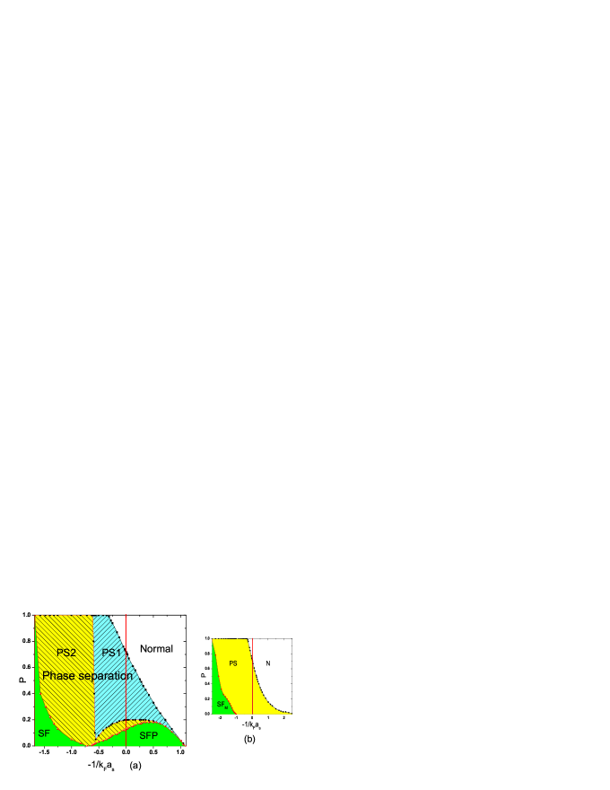
Our findings are dramatically different from those without intra-species correlations, Our proposed phase diagram, Fig. 1a, shows that at T=0, for smaller polarizations, and sufficiently large intra-species correlations, gapped polarized superfluidity (hereafter referred to as SFP) becomes stable on both BCS and BEC sides of the “unitarity” limit. Depending on the inter-species interaction strength, at some polarization, SFP becomes unstable via a 1st-order transition to phase separation, denoted by PS1. PS1 is characterized by a negative “susceptibility”, $\delta P/\delta h$; $P$ being the spin-polarization, and $h$ the difference of the chemical potentials, playing the role of a “magnetic field”. For a given intra-species interaction, and for sufficiently weak inter-species interaction, SFP and PS1 undergo transitions to the normal state on the BCS side. The gapped SFP persists into the BEC regime, sustaining progressively smaller polarizations. Deeper in the BEC regime, we find a superfluid phase (SF) at all polarizations. In the BEC regime, in addition to PS1, we find the existence of a somewhat different phase separated state, PS2, characterized by positive “susceptibility”, but not satisfying requisite superfluid ground state stability criteria.

For our detailed study, we consider a two-species Fermi system with unequal “pseudo-spin” populations. To allow for both inter-species and intra-species correlations, and noting that pseudo-spin rotation invariance would be broken by unequal chemical potentials, we adopt a pairing Hamiltonian given by

$$H = \sum_{k\sigma}\xi_{k\sigma}c_{k\sigma}^{+}c_{k\sigma}$$ (1)

$$+ \sum_{kk^{\prime}q\sigma}\frac{g_{kk^{\prime}}^{\sigma\sigma}}{V}c_{k+q/2\sigma}^{+}c_{-k+q/2\sigma}^{+}c_{-k^{\prime}+q/2\sigma}c_{k^{\prime}+q/2\sigma}$$

$$+ \sum_{kk^{\prime}q}\frac{g_{kk^{\prime}}^{\uparrow\downarrow}}{V}c_{k+q/2\uparrow}^{+}c_{-k+q/2\downarrow}^{+}c_{-k^{\prime}+q/2\downarrow}c_{k^{\prime}+q/2\uparrow}$$

where the pseudospin $\sigma=\uparrow,\downarrow$ denote for example the two hyperfine states of ultracold Fermi atoms. $c_{k\sigma}^{+}$ is the fermion creation operator with kinetic energy $\xi_{k\sigma}=\epsilon_{k\sigma}-\mu_{\sigma}$; $\mu_{\sigma}$ is the chemical potential of each of the species. $g_{kk^{\prime}}^{\uparrow\uparrow}$, and $g_{kk^{\prime}}^{\downarrow\downarrow}$ are the interactions between the up and down spins respectively, and $V$ is the volume. The singlet interaction, $g_{kk^{\prime}}^{\uparrow\downarrow}$ is taken to be a constant, $g_{o}$. This is usually expressed in terms of s-wave scattering length $a_{s}$ using $(4\pi\hbar^{2}a_{s}/m)^{-1}=g_{o}^{-1}+\sum_{k}(2\epsilon_{k})^{-1}$. A mean-field decoupling is attained by introducing three order parameters or gap functions $(\sigma,\sigma^{\prime}=\uparrow,\downarrow)$ given by, $\Delta_{\sigma\sigma^{\prime}}(k,q)=-\sum_{k^{\prime}}g_{kk^{\prime}}^{\sigma\sigma^{\prime}}<c_{-k^{\prime}+q/2\sigma}c_{k^{\prime}+q/2\sigma^{\prime}}>$ This results in a mean-field Hamiltonian given by:

$$H^{MF} = \sum_{k\sigma}\xi_{k\sigma}c_{k\sigma}^{+}c_{k\sigma}-\sum_{k,\sigma}\Delta_{\sigma\sigma}(k,q)c_{k+q/2\sigma}^{+}c_{-k+q/2\sigma}^{+}-\sum_{k,\sigma}\Delta_{\sigma\sigma}^{*}(k,q)c_{-k+q/2\sigma}c_{k+q/2\sigma}-\sum_{k.\sigma}|\Delta_{\sigma\sigma}(k,q)|^{2}/g_{kk}^{\sigma\sigma}$$ (2)

$$- \sum_{k}\Delta_{\downarrow\uparrow}(k,q)c_{k+q/2\uparrow}^{+}c_{-k+q/2\downarrow}^{+}-\sum_{k}\Delta_{\downarrow\uparrow}^{*}(k,q)c_{-k+q/2\downarrow}c_{k+q/2\uparrow}-\sum_{k}|\Delta_{\downarrow\uparrow}(k,q)|^{2}/g_{kk}^{\downarrow\uparrow}$$

We employ the equation of motion method using imaginary time normal and anomalous Matsubara Green’s functions, $G_{\sigma\sigma^{\prime}}(k,\tau)$, $F_{\sigma\sigma^{\prime}}(k,\tau)$, respectively, and our mean-field Hamiltonian, $H^{MF}$. The coupled equations in terms of $\Delta_{\sigma\sigma^{\prime}}$ are given by $G_{\sigma\sigma^{\prime}}(k,\tau)$ and $F_{\sigma\sigma^{\prime}}(k,\tau)$:

$$\partial_{\tau}G_{\sigma\sigma^{\prime}}(k,\tau) = -\delta(\tau)\delta_{\sigma\sigma^{\prime}}-\xi_{k+q/2\sigma}G_{\sigma\sigma^{\prime}}(k,\tau)$$ (3)

$$+\sum_{\sigma^{\prime\prime}}\Delta_{\sigma^{\prime\prime}\sigma}(k,q)F_{\sigma^{\prime\prime}\sigma^{\prime}}(k,\tau)$$

$$\partial_{\tau}F_{\sigma\sigma^{\prime}}(k,\tau) = \xi_{-k+q/2\sigma}F_{\sigma\sigma}(k,\tau)$$ (4)

$$+\sum_{\sigma^{\prime\prime}}\Delta_{\sigma\sigma^{\prime\prime}}^{*}(k,q)G_{\sigma^{\prime\prime}\sigma^{\prime}}(k,\tau)$$

where $\tau$ is the imaginary time variable. These equations may be Fourier transformed in the usual way with $\tau\rightarrow iw_{n}$, $\partial_{\tau}\rightarrow-iw_{n}$, where $iw_{n}=(2n+1)\pi/\beta$ are the Matsubara frequencies, $n$ being an integer and $\beta=1/k_{B}T$.

Here we focus on a superfluid condensate of pairs with zero center-of-mass momentum, $q$. Thus, we do not consider the $q\neq 0$ Fulde-Ferrel-Larkin-Ovchinnikov(FFLO) state Fulde and Ferrell (1964); Larkin and Ovchinnikov (1965), but which may also be studied within this scheme. Solving the Fourier transformed equations at $q=0$, we obtain the 2-point correlation functions:

$$G_{\sigma\sigma^{\prime}}(k,iw_{n}) = \frac{\delta_{\sigma\sigma^{\prime}}f_{\sigma}+\delta_{\sigma-\sigma^{\prime}}(\Delta\Delta_{\uparrow}b_{\downarrow}-\Delta\Delta_{\downarrow}\Delta_{\uparrow})}{D}$$

$$F_{\sigma\sigma^{\prime}}(k,iw_{n}) = \frac{\delta_{\sigma\sigma^{\prime}}f_{\sigma\sigma}+\delta_{\sigma-\sigma^{\prime}}f_{\sigma-\sigma}}{D}$$ (5)

where $f_{\sigma}=\Delta^{2}b_{-\sigma}+\Delta_{-\sigma}^{2}b_{\sigma}-a_{-\sigma}b_{\sigma}b_{-\sigma}$; $f_{\sigma\sigma}=\Delta^{2}\Delta_{-\sigma}+\Delta_{\sigma}\Delta_{-\sigma}^{2}-\Delta_{\sigma}a_{-\sigma}b_{-\sigma}$; $f_{\sigma-\sigma}=\Delta(\Delta^{2}+\Delta_{\sigma}\Delta_{-\sigma}-a_{\sigma}b_{-\sigma})(\delta_{\sigma\downarrow}-\delta_{\sigma\uparrow})$; $D=(\Delta^{2}+\Delta_{\uparrow}\Delta_{\downarrow})^{2}+a_{\uparrow}a_{\downarrow}b_{\uparrow}b_{\downarrow}-\sum_{\sigma}(\Delta^{2}a_{\sigma}+\Delta_{\sigma}^{2}a_{-\sigma})b_{-\sigma}$; with $a_{\sigma}=\xi_{k+q/2\sigma}-iw_{n}$, $b_{\sigma}=-\xi_{-k+q/2\sigma}-iw_{n}$. We have set $\Delta_{\uparrow\uparrow}\equiv\Delta_{\uparrow}$; $\Delta_{\downarrow\downarrow}\equiv\Delta_{\downarrow}$; $\Delta_{\uparrow\downarrow}\equiv\Delta$. The excitation spectrum can be found by examining the poles of the Green’s functions, yielding the quasiparticle energies,

$$E_{k\pm}^{2}=(iw_{n})^{2}=(\alpha\pm\sqrt{\beta})/2$$ (6)

where $\alpha=\xi_{k\uparrow}^{2}+\xi_{k\downarrow}^{2}+2\Delta^{2}+\Delta_{1}^{2}+\Delta_{2}^{2}$, and $\beta=\left[(\xi_{k\uparrow}^{2}-\xi_{k\downarrow}^{2})+(\Delta_{1}^{2}-\Delta_{2}^{2})\right]^{2}+4\Delta^{2}\left[(\xi_{k\uparrow}-\xi_{k\downarrow})^{2}+(\Delta_{1}-\Delta_{2})^{2}\right]$. Various quantities can now be obtained from our 2-point correlation functions. Thus, particle concentrations, $n_{\sigma}$ for the two species ($\sigma=\uparrow,\downarrow$) are given by

$$n_{\sigma} =\sum_{k}\left<c_{k\sigma}^{+}c_{k\sigma}\right>=\sum_{k}\sum_{iw_{n}}\frac{1}{\beta}G_{\sigma\sigma}(k,iw_{n})e^{iw_{n}0^{+}}$$

$$= \sum_{k}\sum_{l=\pm}(-1)^{\lambda}\left[\frac{n_{F}(E_{kl})f_{\sigma}(k,E_{kl})-n_{F}(-E_{kl})f_{\sigma}(k,-E_{kl})}{2E_{kl}(E_{k+}^{2}-E_{k-}^{2})}\right]$$

where $\lambda$ is even for $l=+$, and odd for $l=-$; $n_{F}(E_{kl})$ are the Fermi functions. Likewise the three gaps equations are given by $(\sigma,\sigma^{\prime}=\uparrow,\downarrow)$:

$$\Delta_{\sigma\sigma^{\prime}}=-\sum_{k}g_{kk}^{\sigma\sigma^{\prime}}\sum_{iw_{n}}\frac{1}{\beta}F_{\sigma\sigma^{\prime}}^{*}(k,iw_{n})e^{iw_{n}0^{+}}=-\sum_{k}\sum_{l=\pm}(-1)^{\lambda}g_{kk}^{\sigma\sigma^{\prime}}\left[\frac{n_{F}(E_{kl})f_{\sigma\sigma^{\prime}}(k,E_{kl})-n_{F}(-E_{kl})f_{\sigma\sigma^{\prime}}(k,-E_{kl})}{2E_{kl}(E_{k+}^{2}-E_{k-}^{2})}\right]$$ (8)

The above five equations are coupled, and can be solved self-consistently for the three gap functions, $\Delta,\Delta_{\uparrow},\Delta_{\downarrow}$ for either fixed particle concentrations, $n_{\uparrow}$, $n_{\downarrow}$, or fixed chemical potentials, $\mu_{\uparrow}$, $\mu_{\downarrow}$.

We assume equal masses for the two species, and take the particle spectrum to be $\epsilon_{k}=\hbar^{2}k^{2}/2m$. We adopt standard definitions: polarization, $P=(n_{1}-n_{2})/(n_{1}+n_{2})$; mean chemical potential $\mu=(\mu_{1}+\mu_{2})/2$; chemical potential difference $h=(\mu_{1}-\mu_{2})/2$; Fermi momentum $k_{F\sigma}=(6\pi^{2}n_{\sigma})^{1/3}$. Since $\sum_{k}f(k)\rightarrow\int_{0}^{\infty}f(k)\frac{d^{3}k}{(2\pi)^{3}}\rightarrow\int_{0}^{\infty}k_{F}^{3}f(k/k_{F})\frac{d^{3}(k/k_{F})}{(2\pi)^{3}}$, we can scale quantities having dimension of energy to $\epsilon_{F}$. The inter-species interaction $g_{o}$ is expressed in terms of coupling constant $\eta=-1/(k_{F}a_{s})$. For the intra-species triplet interaction, we take the separable form $g_{kk^{\prime}}^{\sigma\sigma}=g_{1}\omega(k)\omega(k^{\prime})Y_{10}(\hat{k})Y_{10}(\hat{k^{\prime}})$, where we have taken $g_{\uparrow\uparrow}=g_{\downarrow\downarrow}\equiv\tilde{g_{1}}$. More generally the $m=\pm 1$ terms would also be present; however this choice allows us to explore the consequences of intra-species correlations while keeping the calculations tractable. As a check, we also consider different types of momentum dependence: (i) $\omega(k)\propto const$; (ii) $\omega(k)\propto k_{0}k/(k_{0}^{2}+k^{2})$, a generalization of the Nozieres and Schmitt-Rink scheme Noziers and Schmitt-Rink (1985); (iii) $\omega(k)\propto\exp{[-(k/k_{0})^{2}]}$, a Gaussian interaction; $k_{o}$ being a cut-off momentum; these give qualitatively similar behavior. The first two forms of interaction require regularization due to ultraviolet divergence, while the third does not. With regularization, $g_{1}$ can be expressed in terms of a triplet scattering volume $a_{t}$ Iskin and Sa de Melo (2006): $(4\pi\hbar^{2}k_{o}^{2}a_{t}/m)^{-1}=g_{1}^{-1}+\sum_{k}w(k)^{2}/(2\epsilon_{k})$. Thus, $(3n/2\epsilon_{F})\tilde{g_{1}}\equiv g_{1}$ in our plots can be easily expressed in terms of $a_{t}$; e.g. $g_{1}=20$ corresponds to $1/(k_{F}^{3}a_{t})=1.25$.

For arbitrary inter-species s-wave and and intra-species p-wave pairing interactions, and population imbalances, we obtain self-consistent solutions of the $T=0$ gap functions, $\Delta,\Delta_{\uparrow},\Delta{\downarrow}$, and chemical potentials, $\mu_{\sigma}$. On the BCS side, for a given $g_{o}$, the $\uparrow\downarrow$ gap $\Delta$ decreases with increasing intra-species interaction strength $g_{1}$, while at the same time both $\Delta_{\uparrow},\Delta_{\downarrow}$ ($\Delta_{\uparrow}\neq\Delta_{\downarrow}$) increases, crossing at some value of $g_{1}$. The suppression of $\Delta$ is more pronounced at larger polarizations.

A proper construction of the asymmetrical Fermi system phase diagram requires a determination of stable ground states out of the manifold of paired condensates given by our equations Sheehy and Radzihovsky (2006a); Viverit et al. (2000). Accordingly, we carefully consider the stability criteria. The mean-field ground state energy as a function of the gaps at different polarizations, P is given by:

$$E_{G} (\Delta,\Delta_{\uparrow}.\Delta_{\downarrow})=\left<\Psi|H^{MF}|\Psi\right>$$ (9)

$$= E_{o}+\sum_{k\sigma}\left[\xi_{k\sigma}G_{\sigma\sigma}(k,\tau=0^{-})-2\Delta_{\sigma}F_{\sigma\sigma}(k,\tau=0^{-})\right]$$

$$- \sum_{k}2\Delta F_{\downarrow\uparrow}(k,\tau=0^{-})$$

where $E_{o}=-|\Delta_{\uparrow}|^{2}/g_{1}-|\Delta_{\downarrow}|^{2}/g_{1}-|\Delta|^{2}/g_{o}$. To find the stability of the polarized superfluid state SFP, we construct the 3x3 stability matrix out of all partial derivatives $\frac{\partial^{2}E_{G}}{\partial\Delta_{i}\partial\Delta_{j}}$ ($\Delta_{i,j}=\Delta,\Delta_{\uparrow},\Delta_{\downarrow}$), and check for positive definiteness of the determinant of the matrix, and of all its upper-left sub-matrices. We supplement this with analysis of the “susceptibility” $\partial P/\partial h$. Thus, for a given $g_{1}$, the stable polarized superfluid state SFP, in both BCS and BEC regimes, is characterized by $E_{G}$ with a global minimum at non-zero gaps and self-consistently determined values of $\mu_{\sigma}$’s, and $\frac{\partial P}{\partial h}>0$. SFP sustains larger polarizations for progressively larger $g_{1}$.

Similar to the case without intra-species correlations, $g_{1}$, there exists a maximum polarization, $P_{max}$ on the BCS side, beyond which we find no solution to the coupled equations; this determines the SFP/PS1 $\leftrightarrow$ N boundary (Fig. 1a). $P_{max}$ is slightly decreased at unitarity by $g_{1}$. It decreases with increasing $\eta=-1/k_{F}a_{s}$. For a fixed $g_{1}$, close to both BCS and BEC sides of unitarity, and for small polarizations, unlike-spin pairing has appreciable value in the polarized superfluid SFP. However away from unitarity on the BCS side, $\Delta_{\uparrow\downarrow}$ decreases, and $\uparrow\uparrow$ and $\downarrow\downarrow$ pairing becomes more dominant in SFP, as inter-species interaction becomes relatively weak compared to intra-species interaction. On the BEC side away from unitarity, on the other hand, $\Delta_{\uparrow\downarrow}$ is more dominant, and with $\Delta_{\uparrow}$ and $\Delta_{\downarrow}$ becoming negligible, SFP becomes unstable to phase separation, PS2. A SF phase emerges deep in the BCS regime with predominantly unlike-spin pairing at low polarizations and majority spin pairing at higher polarizations.

Figure 2: (Color online) Polarization $P=\frac{n_{\uparrow}-n_{\downarrow}}{n_{\uparrow}+n_{\downarrow}}$ vs $h/\mu=\frac{\mu_{\uparrow}-\mu_{\downarrow}}{\mu_{\uparrow}+\mu{\downarrow}}$ ($h$ acts like a “magnetic field”) for different intra-species strengths $g_{1}$ at a fixed inter-species coupling $\eta=0.25$.

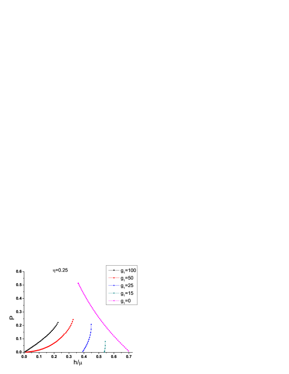
The region PS1 in Fig 1a is characterized by negative “susceptibility”, $\frac{\partial P}{\partial h}$ and doe not satisfy the stability matrix criteria. For a given $P$ and $h$, $E_{G}$ is a maximum at the non-zero gap solutions, separating two local minima – a feature of phase separation into a normal and a superfluid component by 1st-order phase transition. In this context, it is instructive to study $P$ as a function of $h/\mu$ for different values of $g_{1}$, for a fixed $\eta$ (shown in Fig.2 for $\eta=0.25$ (BCS side)). For $g_{1}=g_{1}^{c}\approx 15$, the slope is vertical ($g_{1}^{c}$ is the value of $g_{1}$ at which maximum polarization, $P_{max}$ occurs for a given $\eta$). For $g_{1}\leq g_{1}^{c}$, the slope is negative, corresponding to the BCS superfluid state being unstable to the normal state for $h>\Delta$, but robust against polarization for $h<\Delta$. For $g_{1}>g_{1}^{c}$, the singlet superfluid state can sustain a finite polarization, which exhibits a behavior over the range given by: $P\propto ah+bh^{3}+c$; a,b,c being constants. The linear behavior is achieved for larger values of $g_{1}$, and at low polarizations. In examining $P$ vs $h/\mu$ behavior beyond $P_{max}$, we find, for a given $g_{1}$, two solutions of $P$ corresponding to one value of $h/\mu$. To make a connection to Fig. 1a, obtained for $g_{1}=20$, we note that the allowed range of polarizations for SFP in $P$ vs $h/\mu$ considerations corresponds to the $\eta=0.25$ vertical line, terminating at the SFP-PS1 boundary (Fig 1a). The same line extended from SFP-PS1 boundary to PS1-N boundary correspond to the polarization range bounded by the two solutions of $P$ at a $h/\mu$ in Fig.2. The region PS2 in BEC regime, though characterized by $\frac{\partial P}{\partial h}>0$, is not a stable superfluid phase, since the stability matrix condition cannot be satisfied. The line separating PS1 and PS2 is probably a metastable line, the position of which depends on the p-wave interaction strength.

In summary, we find that the inclusion of intra-species correlations in asymmetrical Fermi systems results in a stable polarized superfluid phase SFP at low polarizations on both BCS and BEC sides of unitarity. We have discussed the nature of the paired states and transition to phase separated states. The SF phase obtained in the deep BEC regime in the case without intra-species correlations, also emerges here with dominant unlike-species pairing, accompanied by weaker majority-species pairing. Our results should be of broad interest as it should be of relevance to any asymmetrical Fermi system, with proper choice of interaction parameters. Here, our choice of parameters appear to agree with cold atom experiment Partridge et al. (2006) that found a SF to PS transition around $\sim 10\%$ polarization around unitarity on the BEC side. Also, the maximum polarization $\sim 70\%$ at unitarity is in agreement with experiments. Further experiments at low polarizations on both sides of unitarity are needed to test our detailed results. Experiments that measure differences in momentum distributions of two species could provide further test. Finally, our phase diagram indicates a tricritical point (SFP,PS1,N phases) at low polarization on the BCS side, in addition to one on the BEC side at $P\sim 1$. This should lead to interesting study of the evolution of these two tricritical points at finite-T; we are exploring these effects.

We would like to thank D. Allender, K. Bedell, J. Engelbrecht, S. Gaudio, R. Hulet, and M. Widom for fruitful comments and discussions. We also acknowledge support from ICAM.

References

- Zwierlein et al. (2006) M. W. Zwierlein, A. Schirotzek, C. H. Schunck, and W. Ketterle, Science 311, 492 (2006).
- Partridge et al. (2006) G. B. Partridge, W. Li, R. I. Kamar, Y. A. Liao, and R. G. Hulet, Science 311, 503 (2006).
- Sarma (1963) G. Sarma, J. Phys. Chem. Solids 24, 1029 (1963).
- Larkin and Ovchinnikov (1965) A. I. Larkin and Y. Ovchinnikov, Sov. Phys. JETP 20 (1965).
- Fulde and Ferrell (1964) P. Fulde and R. A. Ferrell, Phys. Rev. A 135, 550 (1964).
- Takada and Izuyama (1969) S. Takada and T. Izuyama, Prog. Theo. Phys. 41, 635 (1969).
- Suhl et al. (1959) H. H. Suhl, B. T. Matthias, and L. R. Walker, Phys. Rev. Lett. 3, 552 (1959).
- Kondo (1963) J. Kondo, Prog. Theo. Phys. 29, 1 (1963).
- Sedrakian and Lombardo (2000) A. Sedrakian and U. Lombardo, Phys. Rev. Lett. 84, 602 (2000); U. Lombardo, P. Nozieres, P. Schuck, H.-J. Schulze, and A. Sedrakian, Phys. Rev. C 64, 064314 (2001).
- Alford et al. (2001) M. Alford, J. A. Bowers, and K. Rajagopal, Phys. Rev. D 63, 074016 (2001); J. A. Bowers and K. Rajagopal, Phys. Rev. D 66, 065002 (2002); T. Schafer and F. Wilczek, Phys. Rev. D 60, 074014 (1999).
- Bedaque et al. (2003) P. F. Bedaque, H. Caldas, and G. Rupak, Phys. Rev. Lett. 91, 247002 (2003); H. Caldas, Phys. Rev. A 69, 063602 (2004); M. M. Forbes, E. Gubankova, M. V. Liu, and F. Wilczek, Phys. Rev. Lett. 94, 017001 (2005); W. V. Liu and F. Wilczek, Phys. Rev. Lett. 90, 047002 (2003); K. B. Gubbels, M. W. J. Romans, and H. T. C. Stoof (2006).
- Pao et al. (2006) C.-H. Pao, S.-T. Wu, and S.-K. Yip, Phys. Rev. B 73, 132506 (2006); Q. Chen, Y. He, C.-C. Chien, and K. Levin, cond-mat/0608454 (2006); Z.-C. Gu, G. Warner, and F. Zhou, cond-mat/0603091 (2006); M. M. Parish, F. M. Marchetti, A. Lamacraft, and B. D. Simons, cond-mat/0605744 (2006); D. E. Sheehy and L. Radzihovsky, Phys. Rev. Lett. 96, 060401 (2006b).
- Sheehy and Radzihovsky (2006a) D. E. Sheehy and L. Radzihovsky, cond-mat/0608172 (2006a); D. E. Sheehy and L. Radzihovsky, cond-mat/0607803 (2006a).
- Ho and Zhai (2006) T.-L. Ho and H. Zhai, cond-mat/0602568 (2006).
- Huang et al. (2006) X. Huang, X. Hao, and P. Zhuang, cond-mat/0610610 (2006).
- Carlson and Reddy (2005) J. Carlson and S. Reddy, Phys. Rev. Lett. 95, 060401 (2005).
- Bulgac (2006) A. Bulgac, M. M. Forbes,and A. Schwenk, Phys. Rev. Lett. 97, 020402 (2006).
- Quader (1985) K.F. Quader,and K.S. Bedell, J. Low Temp. Phys. 58, 89 (1985).
- Leggett (1980) A. J. Leggett, J. Phys.(Paris) Colloq. 41 (1980).
- Eagles (1969) D. M. Eagles, Phys. Rev. 186, 456 (1969).
- Noziers and Schmitt-Rink (1985) P. Noziers and S. Schmitt-Rink, J. of Low Temp. Phys. 59, 195 (1985).
- Iskin and Sa de Melo (2006) M. Iskin and C.A.R. Sa de Melo, cond-mat/0602157(2006).
- Viverit et al. (2000) L. Viverit, C. J. Pethick, and H. Smith, Phys. Rev. A 61, 053605 (2000).