Rapid granular flows on a rough incline: phase diagram, gas transition, and effects of air drag

Abstract

We report experiments on the overall phase diagram of granular flows on an incline with emphasis on high inclination angles where the mean layer velocity approaches the terminal velocity of a single particle free falling in air. The granular flow was characterized by measurements of the surface velocity, the average layer height, and the mean density of the layer as functions of the hopper opening, the plane inclination angle and the downstream distance $x$ of the flow. At high inclination angles the flow does not reach an $x-$invariant steady state over the length of the inclined plane. For low volume flow rates, a transition was detected between dense and very dilute (gas) flow regimes. We show using a vacuum flow channel that air did not qualitatively change the phase diagram and did not quantitatively modify mean flow velocities of the granular layer except for small changes in the very dilute gas-like phase.

I Introduction

Granular flows are often separated into two categories dealing with (i) dense granular flows where the flow density is not far from the density of static packing (for studies in 2 dimensions see an2001 ; ra2003 ; bede2003 ; ra2004 ; ra2005 or in 3 dimensions see humo1984 ; po1999 ; fopo2001 ; sa1979 ; fopo2003 ; hawa2000 ; gdrmidi2004 ) and (ii) a rapid, very dilute (gas) regime azch1999 , which is often analyzed in terms of a kinetic theory go2003 ). Although flow on a rough inclined plane has become a model experiment because of its simple geometry most of the available research focuses on the dense regime while less data is devoted to characterizing the gas regime and the transition between the dense and very dilute phase regimes.

A granular layer of thickness $h$ on a rough inclined plane starts flowing only if the plane inclination $\theta$ surpasses a critical angle $\theta_{c}$ and stops flowing when $\theta$ is decreased below an angle of repose $\theta_{r}$ (for reviews see: jana1996 ; gdrmidi2004 ; arts2006 ). Experiments in 3 dimensions typically feature a storage container with an opening of height $H$ that influences the volume flow rate of material down the plane po1999 ; fopo2001 ; sa1979 ; fopo2003 ; hawa2000 . The properties of granular flows in this system have been extensively studied when $\theta$ is not much larger than the flow initiation conditions po1999 ; sa1979 ; fopo2003 ; hawa2000 . For $\theta\approx\theta_{r}$ and for small volume flow rates, intermittent flows are observed si2005 including avalanches da2000 and wave-like motion sa1979 ; fopo2003 ; hawa2000 . At somewhat larger $\theta$, the grains flow uniformly with a statistically steady flow velocity that depends on the layer height po1999 ; fopo2003 ; hawa2000 . For still higher $\theta$, the flow properties have not been well studied although an interesting stripe state has been reported fopo2001 ; fopo2002 ; boec2005 . One might expect that the layer density would decrease as $\theta$ is increased because of higher average flow velocity which creates larger shear rates and higher granular temperature. Because the ratio of the down-plane force to the normal force diverges at $\theta=\pi/2$, one might also ask whether a dense phase with a well defined layer thickness continues to exist at large $\theta$.

Flowing granular layers can be described by a set of macroscopic variables that depend on the system control parameters. The two control parameters for granular flow on a rough inclined plane are the hopper opening $H$ and the inclination angle $\theta$. The hopper opening largely influences the volume flow rate from the hopper whereas $\theta$ controls the balance of tangential and normal gravitational force on the layer. An additional parameter that is harder to vary systematically is the roughness of the inclined plane surface. For fixed surface roughness, the flow properties of the layer at fixed $H$ and $\theta$ can be characterized by the surface velocity, the height $h$ and the average density $\rho$. These quantities depend on the control parameters and on each other in a complicated manner. Part of our purpose in this paper is to understand these relationships.

One particular issue for granular flows at high inclination angles was suggested by idealized numerical simulations in which gravitational forcing cannot be balanced by energy dissipation mechanisms, and the flow is predicted to accelerate sier2001 ; sila2003 . Constitutive equations recently proposed for dense granular flows suggest that the effective friction coefficient saturates to a finite value $\mu_{2}$ for high shear rates po1999 ; jofo2005 ; jofo2006 . In this case the flow is expected to accelerate for $\theta$ above $\theta_{2}=$atan$(\mu_{2})$. As we will show in the present work, in accordance with the data presented in po1999 the dense, non-accelerating regime can only be observed up to tan$\theta/$tan$\theta_{2}=0.85$. For the case of density we show, that $\rho$ is observed to decrease substantially from its closed-packed value at plane inclinations starting from tan$\theta/$tan$\theta_{r}=1.45$ (in our case tan$\theta_{2}/$tan$\theta_{r}=1.7$). At very high plane inclinations where a very dilute gas phase is observed the equation of state is certainly much different than for the dense flows and the above criterion is not relevant. For the case of velocity $u$, our characterization of $u$ as a function of downstream distance demonstrates that there is a healing length of order the size of our inclined plane for moderate plane inclinations that complicates a comparison with the predictions for an acceleration threshold. We conclude that because of the limited plane length our data are not complete enough to make a quantitative prediction of the angle up to which stationary flows exist.

As demonstrated in other experiments, air can sometimes have a profound effect on the observed behavior of the granular flow as in, for example, segregation of vertically-vibrated granular materials moch2004 ; moch2005 ; zeho2006 , discharging hourglasses wuma1993 ; muhu2004 , or impact studies lobe2004 . Thus, in order to characterize the properties of granular flow at high inclination angles, it is important to understand how air interacts with the granular flow and to determine the level of fluidization and grain velocity when the role of air drag is no longer negligible.

In this paper, we characterize the flow of relatively mono-dispersed sand particles on a rough inclined plane. The experimental apparatus, that allows for measurements of flow conditions as a function of air pressure, and a characterization of the average terminal velocity of individual grains with different mean sizes and material composition are presented in Sec. II. In Sec. III, we describe our measurements of granular layer velocity, height and density as a function of hopper opening $H$. We summarize our findings in a phase diagram that includes the transition to a gaseous phase. Finally, we conclude with some discussion of the implications and further opportunities for the system of granular flow on an inclined plane.

II Experiment

We start by characterizing the granular material and describing the experimental apparatus used to make quantitative measurements of the flow. For determining the flow properties of the granular layer, we used sand that was sifted with 300 and 500 $\mu$m sieves to yield a mean diameter of $d=400\ \mu$m. We designate this distribution as having a mean of $d=400\ \mu$m and a standard deviation of $50\ \mu$m. We also used finer sand, salt and glass beads to help calibrate the air drag effects.

The experimental setup used for measurements of inclined plane flows is shown in Fig. 1. A glass plate with dimensions 230 cm x 15 cm was set inside a 274 cm long, 20 cm diameter cast-acrylic tube. The leftmost 40 cm of the tube (full with sand in the image) serves as the hopper. The surface of the remaining part (190 cm) of the glass plate was made rough by gluing one layer of grains onto it or by covering the plate with sandpaper that had a characteristic roughness of 190 $\mu$m (80 grit). The same flow regimes were observed for both surfaces. Because the surface of the sandpaper was slightly smoother, we observed a small (about 10$\%$) increase of the flow velocity compared to the case of grains glued onto the plate. The tube was rotatable about the middle so that we could set an arbitrary inclination angle $\theta$. The whole system could be pumped down to $P\approx$ 0.5 mbar.

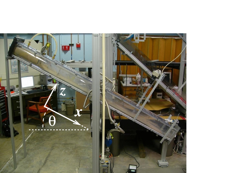
Figure 1: Color online. Photograph of the experimental setup.

The flow velocity $u$ at the surface was determined by analyzing high speed (8000 frames per second) recordings. Space time plots were created by taking one line of the recordings parallel to the main flow. The Fourier transform of such an image (consisting of streaks as traces of particles in the flow) yields the average velocity of surface particles. The thickness of the flow $h$ was monitored by the translation of a laser spot formed by the intersection with the surface of a laser beam aligned at an angle of $20^{o}$ with respect to the inclined plane.

The flow properties were characterized by varying two control parameters: the plane inclination $34.1^{o}<\theta<52.2^{o}$ and the hopper opening $0.4<H<4.4$ cm (i.e. $10<H/d<110$). Setting a constant $H$, we observed a slight increase of the hopper discharge rate when increasing $\theta$, e.g., see Fig. 2. The hopper discharge rate also depended on the presence of air in the system wuma1993 ; vedi1997 ; muhu2004 . In a typical hourglass geometry, when the hopper and the main chamber are separated, the flow of sand faces a counterflow of air as the hopper discharges and a pressure difference builds up. Without a connection between the two chambers in our experiment, the hopper discharge rate was significantly smaller (by about $50\%$) in the presence of air when compared to the case in vacuum. By connecting the two chambers with a flexible tube, the counterflow was substantially reduced, and the discharge rate was about $80-90\%$ of the discharge rate observed in vacuum (Fig. 2). All the measurements presented here were done for the case of reduced counterflow.

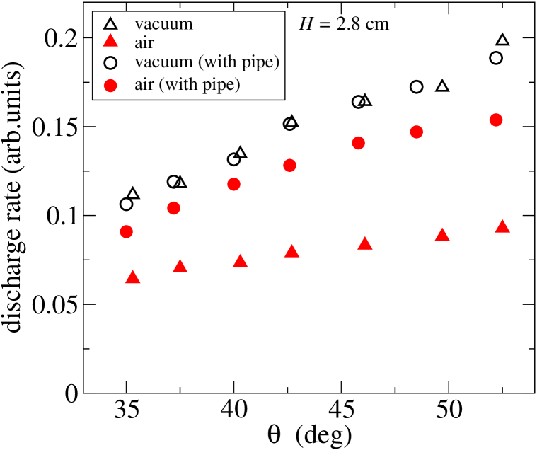
Figure 2: Color online. Hopper discharge rate with $H=2.8$ cm vs. $\theta$ at ambient pressure (filled symbols) and at $P$ = 0.5 mbar (open symbols). The two datasets correspond to the case of two separated chambers (triangles) and reduced counterflow by a connecting pipe (circles).

To set the stage for our discussions of air effects in inclined plane flows, we introduce some results related to the interaction of granular particles with air. One way in which air can affect a granular flow is through the drag force of air acting on an isolated particle. Given a spherical particle of radius $R$ (diameter $d$) and density $\rho_{p}$ falling under gravity $g$ in air with dynamic viscosity $\mu$ and density $\rho_{F}$, the equation of motion is

$${dv\over dt}+{9\mu vc(v)\over 2\rho_{p}R^{2}}=g$$ (1)

where the buoyancy term is ignored since $\rho_{p}>>\rho_{F}$ and $c(v)$ is a turbulent drag correction clgr1978 $c(v)=1+0.15(vd/\nu)^{2/3})$ with $\nu=\mu/\rho_{F}$. The turbulent drag coefficient $c(v)$ yields a good approximation for the range of velocities that are of interest here. The terminal velocity $v_{T}$ is obtained by setting $dv/dt=0$ and solving numerically the equation

$$0.15({2R\over\nu})^{2/3}v^{5/3}+v-{2\over 9}{\rho_{p}R^{2}g\over\mu}=0$$ (2)

The air drag on the individual grains is characterized by the Reynolds number $Re\equiv vd/\nu$ of a particle of diameter $d$ falling at velocity $v$. Taking spherical particles with $R=0.2$ mm and with the density of sand $\rho_{p}=2.5$ g/cm³, by solving Eq. (2) numerically we obtain $v_{T}=3.3$ m/s with a corresponding $Re=90$.

The values of $v_{T}$ were also measured by dropping particles from 2.7 m. All of the particles reached a terminal velocity where the change in their velocities was below $1\%$ over a 7 cm interrogation window. The velocity distribution reflecting the variations in particle size and shape is presented for 100 particles in Fig. 3. The average value of the terminal velocity for the 400 $\mu$m sand is $v_{T}=2.7$ m/s. The measurements were also done for fine sand $d=200\pm 50\ \mu$m, salt $d=400\pm 50\ \mu$m and glass beads $d=510\pm 50\ \mu$m, yielding the the velocity distributions presented in Fig. 3. The corresponding mean values of $v_{T}$ are $1.8$ m/s, $3.0$ m/s and $4.0$ m/s, respectively. The calculated values of $v_{T}$ are indicated with a vertical line for each case. The calculated values of $v_{T}$ are close to the measured values with deviations between data and theory presumably resulting from non-spherical shapes and/or uncertainties in the mean particle diameter. For example, the deviations observed for the two sets of sand can be consistently explained with non-centered size distributions.

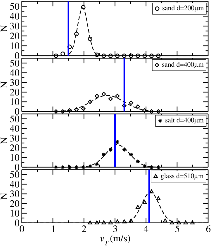
Figure 3: Color online. Distribution of experimental values of $v_{T}$ for different granular materials: fine sand ($d=200\pm 50\ \mu$m), sand ($d=400\pm 50\ \mu$m), salt ($d=400\pm 50\ \mu$m), and glass beads ($d=510\pm 50\ \mu$m). The dashed lines are Gaussian fits to the data, and the solid vertical lines are the calculated values of $v_{T}$.

Having determined that our calculation of $v_{T}$ agrees well with the measured data, we used Eq. 2 to estimate the air drag reduction and the resulting increase in $v_{T}$ as a function of air pressure. The dynamic viscosity $\mu$ of air is almost constant as a function of air pressure $P$. Using an ideal gas relationship between $\rho_{F}$ and P and Eq. 2, one obtains $v_{T}$ (and $Re$) as a function of $P$. As seen in Fig. 4, $v_{T}$ is expected to increase by a factor of 4 when $P$ decreases to 0.5 mbar. If air drag plays a significant role in determining the granular flow state, the substantial decrease in air drag under vacuum will reveal that effect. Here we ignore the expected further increase in the terminal velocity at very low pressures when the air mean free path is comparable to the particle diameter.

Figure 4: Calculated terminal velocity of spherical particles with $d=400\ \mu$m and $\rho=2.5$ g/cm³ vs. $P$.

Another approach to estimating the effect of air drag on a flowing granular layer is to assume that the granular layer is similar to a fluid and that the air forms a boundary layer between air at large distance with zero velocity and the granular layer flowing with a “surface velocity” $v$. A Prandtl boundary layer description yields a boundary layer thickness $\delta=3.4(\nu x/v)^{1/2}$ where $x$ is the downstream distance. The force per unit area $f_{A}$ exerted on the flow by the entrained air is approximately $0.66\ (\rho_{F}\mu v^{3}/x)^{1/2}$. The relevant parameters of the air are $\mu=1.789\ \cdot 10^{-5}$ Pa s, $\rho_{F}=0.96$ kg/m³ (for local pressure $P\approx 0.76P_{ATM}$), and $\nu=0.19$. Taking a distance $x=100$ cm and $v=300$ cm/sec, one obtains $\delta\approx 0.2$ cm and $f_{A}\approx 0.01$ N/m² which is less than 0.1$\%$ of the gravitational force $-$ a negligible effect. The surface of a granular flow, however, is not as sharply defined as it is for liquid flows. If there were substantial fluidization of the granular layer, the cumulative drag force experienced by the low density particles might play a role in the instabilities of the homogeneous flow.

III Results and Discussion

III.1 Phase diagram

Based on qualitative observations of the flow and on quantitative measurements presented below, we can separate the granular flow into regions with certain characteristic features. Such a phase diagram identifying the different flow regimes as a function of the two control parameters $H$ and $\theta$ is shown in Fig. 5. The ratios tan$\theta$/tan$\theta_{r}$ and $H/d$ are also shown on the top and right axes, respectively, where $\theta_{r}=30.5$ is the independently measured bulk angle of repose for the granular material used here. The boundaries are neither precisely defined nor indicative of sharp transitions between different flow regimes. Further, this phase diagram does not capture the convective nature of the granular flow in that features or flow properties may evolve over length scales comparable to the length of the inclined plane. Nevertheless, identification of the general regimes are useful in setting the stage for more complex issues raised below.

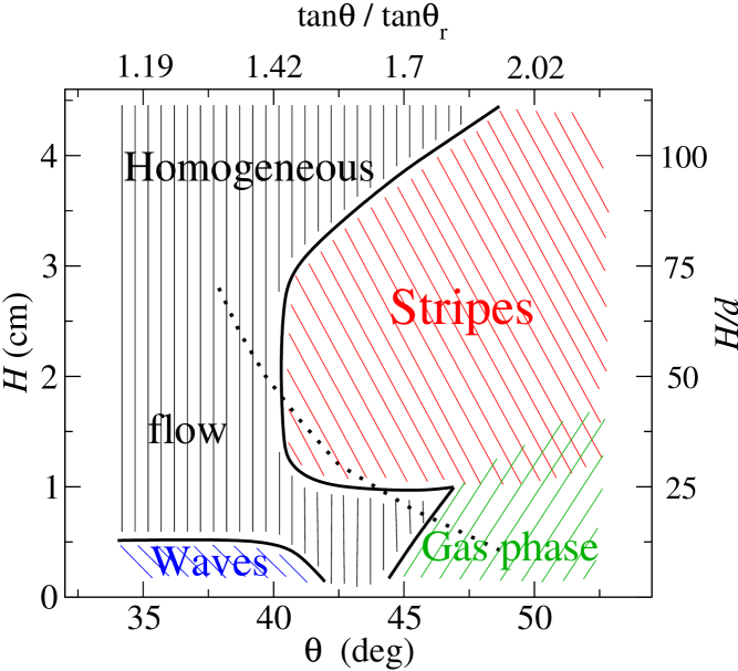
Figure 5: Color online. Phase diagram of the flow regimes in the phase space defined by $H$ and $\theta$. The dotted line divides the diagram into two regions: low flow rates and not too steep planes where $x-$invariant steady flow is observed and higher flow rates and faster flows where the flow is still accelerating as measured at $x=1$ m. The ratios $\tan\theta/\tan\theta_{r}$ and $H/d$ are labeled on the top and right axes, respectively.

At very slow flow rates and low plane inclinations the homogeneous flow is unstable and organizes itself into waves. The properties of such waves have been studied extensively fopo2003 . By increasing the flow rate and staying in the range of not very steep plane inclinations (up to about $40^{o}$), the flow becomes homogeneous. For steeper planes an instability occurs leading to a pattern consisting of lateral stripes fopo2001 ; fopo2002 . A detailed characterization of the stripe state in our system will be presented elsewhere boec2005 . The dashed line divides the diagram into two regions: accelerating and $x-$invariant steady flows. Above the dashed line the acceleration of the flow (averaged over the range of $60<x<140$ cm) was more than 5% of g sin$\theta$. This boundary depends on the distance downstream $x$ at which the acceleration was measured as discussed in more detail in Sec. III.3. The phase diagram was found to be qualitatively the same for flow at ambient pressure and flow at low pressure with $P=0.5$ mbar.

III.2 Flow thickness and density

In this section, we describe our procedure for measuring layer height and mean density of the flowing layer. The flow thickness was measured by laser deflection.

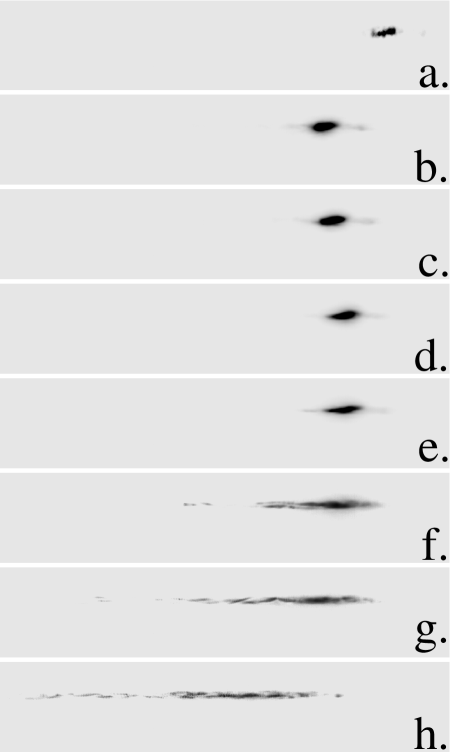
Figure 6: Image of the laser spot for (a) no flow and for flow at inclination angles $\theta$ of (b) $35.0^{o}$, (c) $37.2^{o}$, (d) $40.0^{o}$, (e) $42.6^{o}$, (f) $45.8^{o}$, (g) $48.5^{o}$ and (h) $52.2^{o}$. $H=0.4$ cm and $x=79$ cm.

The plane of the images shown in Fig. 6 was parallel to the inclined plane. A laser beam projected from the left hand side of the image at an angle of $20^{o}$ with respect to the plane of the image produced a localized laser spot. The first image, Fig. 6a, shows the case of the empty chamber without flow, where the laser beam was reflected by the rough surface of the inclined plane. The other images (b-h) were taken in the presence of flow at a constant hopper opening $H=0.4$ cm and downstream distance $x=79$ cm with increasing $\theta$ as we go from (b-h). The laser beam was reflected from the particles at the surface of the flowing layer. The horizontal shift of the laser spot with respect to image (a) measured the thickness of the flowing layer. This measurement is straightforward when the laser spot did not change its shape, i.e., the surface of the flow was well defined (Figs. 6b-e). The first sign of decreasing flow density can be seen in Fig. 6f where the shape of the reflected laser spot changed significantly. The spot spreading became more pronounced with increasing $\theta$ (Figs. 6g-h).

To get a better measure of the flow thickness in this regime the light intensity $I$ detected at a height $z$ above the inclined plane was integrated over 200 equally-spaced images taken over a time period of 3.3 s. The $I(z)$ curves are shown in Fig. 7 corresponding to the last four plane inclinations of Fig. 6. Because of the increasing fluctuations in the laser spot intensity for the higher $\theta$, averaging over many images was necessary.

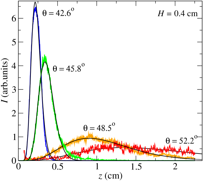
Figure 7: Color online. Time-averaged light intensity I(z) vs. $z$ for $\theta$ values indicated. $H=0.4$ cm, $x=155$ cm. Solid lines are curve fits of the form $az^{b}e^{-cz}$.

For the relatively dense regime (with a compact laser spot), the position of the center of mass of the laser spot was taken as the flow thickness $h$. In the very dilute regime we integrate the $I(z)$ curves and define $h$ as the height below which 80$\%$ of the flowing grains were detected.

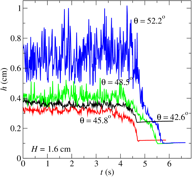
Figure 8: Color online. Flow thickness $h$ vs. $t$ for plane inclinations $\theta=42.6^{o}$, $45.8^{o}$, $48.5^{o}$ and $52.2^{o}$. $H=1.6$ cm, $x=155$ cm. Flow was stopped at $t\approx 4$ s.

The flow density was measured in the following manner. A stationary flow was established and was maintained for about 4 seconds. The flow was then “frozen” by rapidly decreasing the plane inclination.

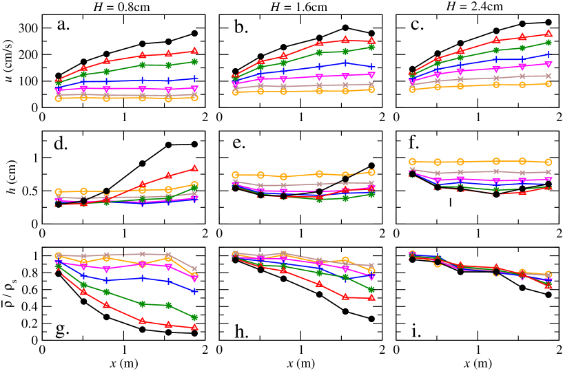
Figure 9: Color online. Velocity $u$ (a-c) thickness $h$ (d-f) and calculated normalized flow density $\overline{\rho}/\rho_{s}$ (g-i) as a function of $x$ the distance measured from the hopper gate for three values of the hopper opening $H=0.8$ cm, $H=1.6$ cm and $H=2.4$ cm. The symbols correspond to the plane inclinations $\theta$ of $35.0^{o}$ ($\circ$), $37.2^{o}$ (x), $40.0^{o}$ ($\nabla$), $42.6^{o}$ (+), $45.8^{o}$ ($\star$), $48.5^{o}$ ($\triangle$) and $52.2^{o}$ ($\bullet$).

The time evolution of the center of mass of the laser spot is shown in Fig. 8 for the same set of plane inclinations as in Fig. 7. The flow height fluctuated in the first 4 seconds with larger fluctuations in $h$ for higher values of $\theta$. As the flow stopped, the height dropped to the height corresponding to the static (nearly random closed packed) material. The height change between the stationary flow and the frozen state reflected the mean density change which became larger with increasing $\theta$, see Fig. 8. The ratio of the static height and the height of the stationary flow gives the normalized depth-averaged density of the flow $\overline{\rho}/\rho_{s}$, where $\rho_{s}$ is the static density. This measurement of height and density averages over some distance in $x$ because the flow does not stop instantaneously. Assuming an exponential decay of the velocity and a total stopping time of about 0.5 sec from the data in Fig. 7, one obtains an averaging length of between 10 and 50 cm. Below we describe a more local albeit less precise measure of density derived from measurements of $u$ and $h$.

III.3 Flow characterization as a function of $\theta$

Granular material exits the hopper at low velocity with height $H$ and a density $\rho_{s}$ that is close to that of a random close-packed state. The material accelerates, thins and becomes less dense as the interaction of the grains with the rough bottom surface partially fluidizes the granular state. At low inclination angles, the system reaches an an $x-$invariant steady state after some healing length $\xi$ where layer height $h$, mean velocity $u$, and mean density $\rho$ do not change with downstream distance $x$. For $\theta$ larger than about $40^{o}$, the flow is not stationary as a function of $x$ and more complicated states are observed. The flow appears to become stationary on healing lengths of order the plane length $L$ for large values of $\theta$ as described below.

All measurements of $u$ and $h$ were repeated at six locations at a distance $x$ measured from the hopper in the range of $20$ cm $<x<187$ cm. The flow velocity $u$ and layer height $h$ are shown as functions of $x$ for three hopper openings $H=$ 0.8 cm, 1.6 cm and 2.4 cm in Figs. 9a-f.

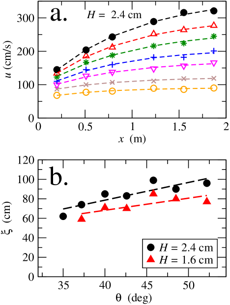
Figure 10: Color online. (a) Fits to the $u(x)$ data taken at $H=2.4$ cm. The symbols correspond to the plane inclinations $\theta$ of $35.0^{o}$ ($\circ$), $37.2^{o}$ (x), $40.0^{o}$ ($\nabla$), $42.6^{o}$ (+), $45.8^{o}$ ($\star$), $48.5^{o}$ ($\triangle$) and $52.2^{o}$ ($\bullet$). (b) Healing length $\xi$ as a function of $\theta$ for $H=1.6$ cm and $H=2.4$ cm.

For higher plane inclinations the flow did not reach a stationary state over the plane length $L$. The evolution of the granular flow can be partially understood by an analysis of $u$ as a function of downstream distance $x$ for different $\theta$. The flow is driven by the gravitational force $\rho g\sin\theta$ and damped by dissipation forces, e.g., friction and/or inelastic collisions. In the simplest approach we can assume that the flow would approach a terminal velocity $u_{f}$ like $u(x)=u_{f}-(u_{f}-u_{0})e^{-x/\xi}$ where $\xi$ corresponds to the healing length of the flow. Fitting the data in Fig. 9a-c to this form allows for the determination of $\xi$ and the velocities $u_{0}$ and $u_{f}$ for different $H$ and $\theta$. In Fig. 10a, we show data for $u$ and fits to the exponential form. The data are well fit by exponential saturation. The resulting values of $\xi$ are shown in Fig. 10b. as a function of $\theta$ for $H=1.6$ cm and $H=2.4$ cm. The healing lengths are of order $L/2$ for $\theta>43^{o}$. Because the data show little variation with $x$ for smaller $\theta$, our fits almost certainly overestimate $\xi$ in that region.

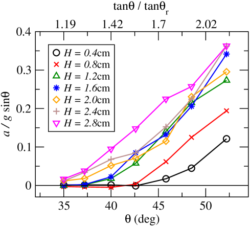
Figure 11: Color online. Acceleration averaged over $60<x<140$ cm for $H$ values of 0.4 cm ($\circ$), 0.8cm (x), 1.2 cm ($\triangle$), 1.6 cm ($\star$), 2.0 cm ($\diamond$), 2.4 cm (+) and 2.8 cm ($\nabla$).

From information about the surface velocity $u$ and the layer thickness $h$, additional information can be inferred about the granular layer despite the inability to directly measure the $z$ dependence of density and velocity. If we assume that the $u(z)$ and $\rho(z)$ profiles do not change their character along $x$, then by conservation of mass one has that the mass flux per unit channel width is $F=h\overline{\rho u}$ where the overbar denotes a depth average. Numerical simulations sier2001 suggest that for at least some range of $\theta$, $\rho$ is almost constant over the depth. With that assumption, we have that $F\approx\overline{\rho}h\overline{u}$. Thus, as a first approximation, plotting $F/uh$ as a function of $x$ provides information about the downstream evolution of the mean density $\overline{\rho}$. The degree to which this is a good approximation depends on the details of $\rho(z)$ and $u(z)$. The slight difference in $\overline{\rho}$ between the values estimated this way and measured by a more precise method presented Sec. III.2, can result from a nonuniform ($z$ dependent density) at faster flows. Because we do not know the absolute value for $F$, we normalize the resulting values of $\overline{\rho}$ assuming that the flow density for the lowest plane inclination was near to the density of the static packing $\rho_{s}$ near the hopper. For the other values of $\theta$ we assumed a $60\%$ increase of the hopper flow rate between $\theta=35.0^{o}-52.2^{o}$ for all values of $H$. The resulting normalized mean density $\overline{\rho}/\rho_{s}$ is shown in Figs. 9g-i as a function of $x$. One sees that the density drops rapidly as a result of increasing velocity for higher plane inclinations especially for the case of lower incoming flow rates. A more precise characterization of the density change using the method described in Section III.2, made at one downstream location $x=155$ cm, will be presented below. Results of the two methods agree within the uncertainties inherent in each approach.

Using the $u(x)$ curves the acceleration of the flow was obtained by assuming that $a=du/dt\approx udu/dx$. The average value of $a$ over the range 60 cm $<x<$ 140 cm is presented as a function of $\theta$ in Fig. 11. At higher plane inclinations, there is a significant acceleration for each value of $H$ whereas for the lowest value of $\theta$ the flow is $x-$invariant for all the $H$ values we investigated. The value of $H$ corresponding to $a=0.05g\sin\theta$ is indicated as a function of $\theta$ in Fig. 5 with a dotted line as a boundary between the accelerating and $x-$invariant steady regimes measured at this distance from the hopper.

In the following we analyze the velocity $u$, flow thickness $h$ and dimensionless mean flow density $\overline{\rho}/\rho_{s}$ as a function of $\theta$ and $H$ at the location $x=155$ cm below the hopper. Parts of our data correspond to accelerating non-stationary flow. Since we are reporting averages obtained near the channel center, we need to determine the degree to which those averages depend on the lateral homogeneity of the flow. Thus, we first indicate some measure of the lateral flow structure.

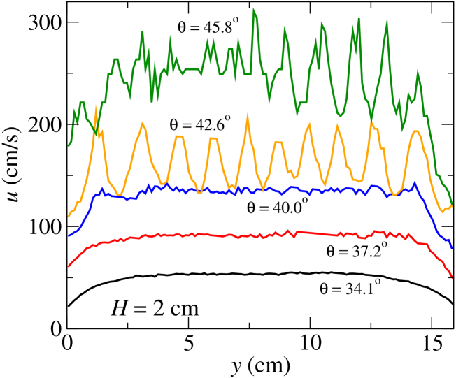
Figure 12: Color online. Surface velocity profiles $u(y)$ of the flow for plane inclinations of $\theta=34.1^{o}$, $37.2^{o}$, $40.0^{o}$, $42.6^{o}$ and $45.8^{o}$. The data were taken the location $x=155$ cm below the hopper at $H=2.0$ cm.

Lateral velocity profiles $u(y)$ are presented in Fig. 12. In the homogeneous dense flow regime, the velocity is relatively constant over the center 12 cm of the channel corresponding to about 75% of the channel width. At the edges of the channel there are boundary layers that arise from the friction with the sidewalls. As the sidewalls of the channel have a smooth surface, friction is significantly less important there when compared to the rough plane. The transition to the stripe state (see curves in Fig. 12 with $\theta$ values of 42.6^o and 45.8^o) happens at around $\theta=41^{o}$.

The surface flow velocity $u$, the height of the flowing layer $h$ and its standard deviation defined as $\sigma=\sqrt{\frac{\int I(z)(z-h)^{2}dz}{\int I(z)dz}}$ are shown as a function of $H$ in Fig. 13 as measured at $x=155$ cm.

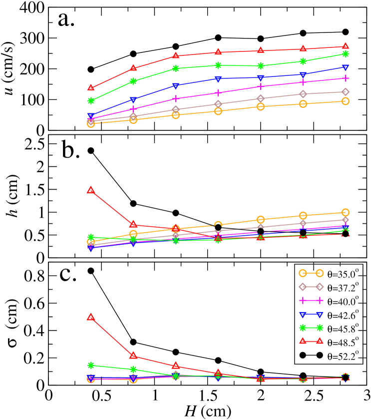
Figure 13: Color online. The flow velocity $u$, layer thickness $h$ and its standard deviation $\sigma_{h}$ vs. $H$ at $x=155$ cm.

The flow velocity is a monotonically increasing function of $H$ for all plane inclinations. In the fluid-like regime $h$ is a monotonically increasing function of $H$ as well, whereas $\sigma$ has a constant low value reflecting the constant shape of the laser spot. The sign of the transition into the gaseous phase is the rapid increase of $h$ and $\sigma$ with decreasing $H$ at higher plane inclinations.

The same set of data for $u$, $h$ and $\sigma$ is presented in Fig. 14 as a function of $\theta$. Again $u$ is a monotonically increasing function of $\theta$ for each value of $H$. In the fluid-like regime (larger values of $H$) the slope of the $u(\theta)$ curves is nearly constant. At smaller $H$ the slope increases considerably when entering the gaseous regime. The flow thickness $h$ decreases with increasing $\theta$ in the fluid-like regime meaning that larger flow velocity results in smaller flow thickness. This effect is actually stronger than Fig. 14b indicates, as the incoming flow rate slightly increases with increasing $\theta$ (see Fig. 2). Thus, thinning of the flow as a result of larger flow velocities is slightly counterbalanced by the growing value of the flow rate by increasing $\theta$.

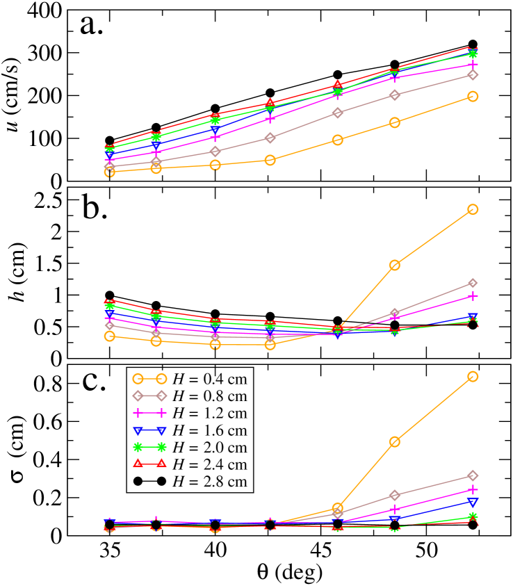
Figure 14: Color online. The flow velocity $u$, flow thickness $h$ and its standard deviation $\sigma_{h}$ as a function of $\theta$ at $x=155$ cm.

The different flow regimes can best be characterized by the flow density. As we see in Fig. 15 the normalized mean density $\overline{\rho}/\rho_{s}$ drops continuously with increasing $\theta$. The density drop is more dramatic for smaller incoming flow rate than for thicker flows.

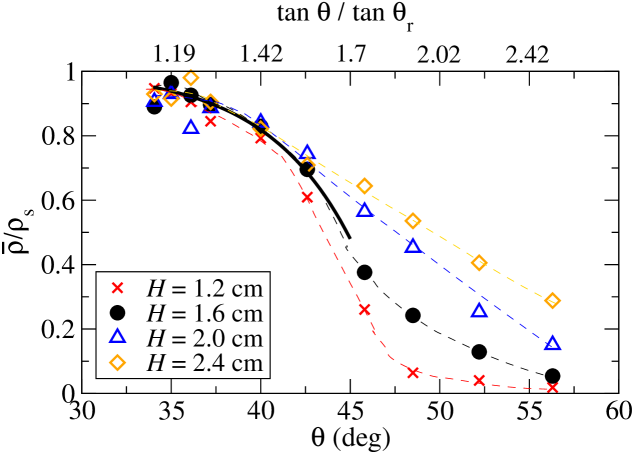
Figure 15: Color online. Normalized mean density $\overline{\rho}/\rho_{s}$ as a function of $\theta$ for $H=1.2$ cm (x), $1.6$ cm ($\bullet$), $2.0$ cm ($\triangle$) and $2.4$ cm ($\diamond$) at $x=155$ cm. The dashed lines are guides to the eye, while the continous line corresponds to $\rho/\rho_{s}=1-0.52\cdot$tan${}^{6}\theta$.

The first regime corresponds to dense flows (slightly above the angle of repose) and is often characterized by the Pouliquen flow rule, where the depth averaged velocity $\overline{u}$ is proportional to $h^{3/2}$ po1999 ; fopo2003 . This regime is reported to exist for the plane inclinations $\tan\theta/\tan\theta_{r}<1.45$, and the dense flow can be unstable with respect to the formation of waves fopo2003 . According to our measurements the mean density in this regime is slightly decreasing with $\theta$ but always stays larger than $\overline{\rho}/\rho_{s}=0.8$. According to a recent theory by Jenkins je2006 the density should decrease as $\rho/\rho_{s}=1-B\cdot$tan${}^{6}\theta$. A reasonable fit is obtained by this formula for a range of $H$ up to the plane inclination $\tan\theta/\tan\theta_{r}<1.5$ yielding $B=0.52$. In the second regime falling in the range of $1.45<\tan\theta/\tan\theta_{r}<2.4$, a stripe pattern can be observed with an average density of $0.2<\overline{\rho}/\rho_{s}<0.8$. The detailed characterization of the stripe structure is beyond the scope of this paper. In the third regime, the stripe structure disappears as the flow gets very fluidized with an average density of $\overline{\rho}/\rho_{s}<0.2$. A dramatic density decrease was observed for lower incoming flow rates, typically at $\tan\theta/\tan\theta_{r}>1.6$, yielding a gas-like phase where the density was less than $5\%$ of $\rho_{s}$. We characterize this transition in more detail below.

The surface flow velocity $u$ as a function of height $h$ is presented in Fig. 16a for the fluid-like regime. Note that only the first curve (at $\theta=35.0^{o}$) corresponds to stationary flows, the other curves (partly) fall already in the range of accelerating flows. Two sets of data were taken: (i) in the presence of air (filled symbols) and (ii) at low pressure $P=0.5$ mbar (open symbols). In this regime the two sets of data match implying that air drag does not become important even at the fastest flows where the grain velocity is close to the value of the terminal velocity measured in free fall.

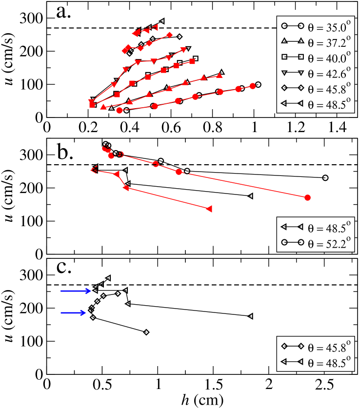
Figure 16: Color online. The flow velocity $u$ vs. $h$ for a set of plane inclinations in the presence of air (filled symbols) and in vacuum (open symbols) in the (a) fluid-like phase, (b) gaseous phase. The transition between the above regimes is indicated in (c) by horizontal arrows. Data taken at $x=155$ cm. The horizontal dashed lines correspond to $v_{T}$.

In the gaseous regime, however, (see Fig. 16b) particle velocities measured at ambient pressure are slightly smaller than at low pressure. Thus, in the gas phase the average interparticle distance is considerably increased and the contribution of air drag to the dissipation becomes important.

The changing nature of the flow is visualized in Fig. 16c where all the data points are presented for two plane inclinations for the two regimes and the transition between them. The sharply different tendency of the $u(h)$ curves in Fig. 16a and Fig. 16b reflects the nature of the transition between the fluid-like and gaseous phases. For $\theta=48.5^{o}$ the larger flow rates give rise to dense flows (Fig. 16a) where increasing $H$ leads to increasing $h$ and faster flow. At lower values of the hopper flow rate decreasing $H$ leads to increasing levels of fluidization and to a transition to the gaseous phase. In this regime, see Fig. 16b, the density of the flow rapidly decreases with decreasing $H$ and the measured thickness rapidly increases. Contrary to trends for the fluid-like phase, the leftmost data points of the curves in Fig. 16b correspond to the highest hopper flow rates and the rightmost ones to the lowest hopper flow rate. Thus, the flow is not simply determined by ($\theta$, $h$, $x$) as is the case for dense flows. For a given $h$, $\theta$ and $x$, two solutions exists, one corresponding to a dense phase and the other to a very dilute one, depending on the flow rate.

A recent linear stability analysis indicated, that the air drag could play a role in the development of stripe patterns in the fluid-like regime arts2006 ; ar2004 . According to our findings the density of the flow for the stripe state was in the range of $0.2<\overline{\rho}/\rho_{s}<0.8$, corresponding to the regime where the role of the air drag is minor. The flow properties are not affected even at flow velocities near the terminal velocity in free fall. At the transition to the gaseous state the stripes disappear and the rapid decrease of the flow density leads to visible effects of air drag.

In summary, we have presented a detailed description of granular flow on a rough inclined plane - one of the most commonly used model systems for granular dynamics - concentrating on the fast flow regime. We developed a method to measure the depth averaged normalized flow density $\overline{\rho}/\rho_{s}$ and characterized the flow regimes as a function of $\overline{\rho}/\rho_{s}$. We have characterized the transition to a very dilute gaseous phase that takes place by increasing plane inclination and decreasing incoming flow rate. By measuring the flow properties at ambient pressure and at low pressure ($P\approx 0.5$ mbar) in a vacuum flow channel we have shown that the dissipation by the air drag (with respect to the other dissipational processes) is non-negligible only in the dilute gas-like phase. Other implications of this work involves the possibility of linking changes in the flow structure (such as the stripe state) as a function of plane inclination to the change in the depth averaged normalized flow density $\overline{\rho}/\rho_{s}$.

This work was funded by the US Department of Energy (W-7405-ENG). The authors benefited from discussions with I.S. Aranson. T.B. acknowledges support by the Bolyai János Scholarship of the Hungarian Academy of Sciences and the Hungarian Scientific Research Fund (Contract No. OTKA-F-060157).

References

- (1) C. Ancey, Phys. Rev. E 65, 011304 (2001).
- (2) J. Rajchenbach, Phys. Rev. Lett. 90, 144302 (2003).
- (3) G. Berton, R. Delannay, P. Richard, N. Taberlet and A. Valance, Phys. Rev. E 68, 051303 (2003).
- (4) J. Rajchenbach, J. Phys.: Condens. Matter 17, S2731 (2005).
- (5) J. Rajchenbach, Eur. Phys. J. E 14, 367 (2004).
- (6) GDR MiDi, Eur. Phys. J. E 14, 341 (2004).
- (7) O. Hungr and N.R. Morgenstern, Géotechnique 34, 405 (1984).
- (8) Y. Forterre and O. Pouliquen, Phys. Rev. Lett. 86, 5886 (2001).
- (9) O. Pouliquen, Phys. of Fluids 11, No.3, 542 (1999).
- (10) Y. Forterre and O. Pouliquen, J. Fluid Mech. 486, 21 (2003).
- (11) S.B. Savage, J. Fluid Mech. 92, 53 (1979).
- (12) D.M. Hanes and O.R. Walton, Powder Technology 109, 133 (2000).
- (13) E. Azanza, F. Chevoir and P. Moucheront, J. Fluid. Mech. 400, 199 (1999).
- (14) I. Goldhirsch, Ann. Rev. Fluid. Mech. 35, 267 (2003).
- (15) H.M. Jaeger, S.R. Nagel and R.P. Behringer, Rev. Mod. Phys. 68 1259 (1996).
- (16) I.S. Aranson and L.S. Tsimring, Rev. Mod. Phys. 78 641 (2006).†
- (17) L.E. Silbert, Phys. Rev. Lett. 94, 098002 (2005).
- (18) A. Daerr, Ph.D. thesis, University of Paris VII (France), (2000).
- (19) Y. Forterre and O. Pouliquen, J. Fluid Mech. 467, 361 (2002).
- (20) T. Börzsönyi and R.E. Ecke, Unpublished.
- (21) L.E. Silbert, D. Ertas, G.S. Grest, T.C. Halsey, D. Levine and S.J. Plimpton, Phys. Rev. E 64, 051302 (2001).
- (22) L.E. Silbert, J.W. Landry and G.S. Grest, Phys. of Fluids 15, 1 (2003).
- (23) P. Jop, Y. Forterre and O. Pouliquen, J. Fluid Mech., 541, 167 (2005).
- (24) P. Jop, Y. Forterre and O. Pouliquen, Nature, 441, 727 (2006).
- (25) M.E. Möbius, X. Cheng, G.S. Karczmar, S.R. Nagel and H.M. Jaeger, Phys. Rev. Lett. 93, 198001 (2004).
- (26) M.E. Möbius, X. Cheng, P. Eshuis, G.S. Karczmar, S.R. Nagel and H.M. Jaeger, Phys. Rev. E 72, 011304 (2005).
- (27) C. Zeilstra, M.A. van der Hoef, and J.A.M. Kuipers, Phys. Rev. E 74, 010302(R) (2006).
- (28) X-I. Wu, K.J. Maloy, A. Hansen, M. Ammi, and D. Bideau, Phys. Rev. Lett. 71, 1363 (1993).
- (29) B.K. Muite, M.L. Hunt, and G.G. Joseph Phys. of Fluids 16, 3415 (2004).
- (30) D. Lohse, R. Bergmann, R. Mikkelsen, C. Zeilstra, D. van der Meer, M. Versluis, K. van der Weele, M. van der Hoef and H. Kuipers Phys. Rev. Lett. 93, 198003 (2004).
- (31) C. T. Veje and P. Dimon, Phys. Rev. E 56, 4376 (1997).
- (32) R. Clift, J.R. Grace, and M.E. Weber, Bubbles, Drops, and Particles (Academic Press, New York, 1978).
- (33) J.T. Jenkins, Phys. of Fluids 18, 103307 (2006).
- (34) I.S. Aranson, private communication, (2004).