Quantum Spin Hall Effect and Topological Phase Transition in HgTe Quantum Wells

We show that the Quantum Spin Hall Effect, a state of matter with topological properties distinct from conventional insulators, can be realized in HgTe/CdTe semiconductor quantum wells. By varying the thickness of the quantum well, the electronic state changes from a normal to an “inverted” type at a critical thickness $d_{c}$. We show that this transition is a topological quantum phase transition between a conventional insulating phase and a phase exhibiting the QSH effect with a single pair of helical edge states. We also discuss the methods for experimental detection of the QSH effect.

The spin Hall effect (?, ?, ?, ?, ?) has attracted great attention recently in condensed matter physics both for its fundamental scientific importance, and its potentially practical application in semiconductor spintronics. In particular, the intrinsic spin Hall effect promises the possibility of designing the intrinsic electronic properties of materials so that the effect can be maximized. Based on this line of reasoning, it was shown (?) that the intrinsic spin Hall effect can in principle exist in band insulators, where the spin current can flow without dissipation. Motivated by this suggestion, the quantum spin Hall (QSH) effect has been proposed independently both for graphene (?) and semiconductors (?, ?) , where the spin current is carried entirely by the helical edge states in two dimensional samples. Time reversal symmetry plays an important role in the dynamics of the helical edge states (?, ?, ?). When there are an even number of pairs of helical states at each edge, impurity scattering or many-body interactions can open a gap at the edge and render the system topologically trivial. However, when there are an odd number of pairs of helical states at each edge these effects cannot open a gap unless time reversal symmetry is spontaneously broken at the edge. The stability of the helical edge states has been confirmed in extensive numerical calculations (?, ?). The time reversal property leads to the $Z_{2}$ classification (?) of the QSH state. States of matter can be classified according to their topological properties. For example, the integer quantum Hall effect is characterized by a topological integer $n$ (?), which determines the quantized value of the Hall conductance and the number of chiral edge states. It is invariant under smooth distortions of the Hamiltonian, as long as the energy gap does not collapse. Similarly, the number of helical edge states, defined modulo two, of the QSH state is also invariant under topologically smooth distortions of the Hamiltonian. Therefore, the QSH state is a topologically distinct new state of matter, in the same sense as the charge quantum Hall effect.

Unfortunately, the initial proposal of the QSH in graphene (?) was later shown to be unrealistic (?, ?), as the gap opened by the spin-orbit interaction turns out to be extremely small, of the order of $10^{-3}$ meV. There are also no immediate experimental systems available for the proposals in Ref.  (?, ?). Here, we present theoretical investigations of the type-III semiconductor quantum wells, and show that the QSH state should be realized in the “inverted” regime where the well thickness $d$ is greater than a certain critical thickness $d_{c}$. Based on general symmetry considerations and standard $k\cdot p$ perturbation theory for semiconductors (?), we show that the electronic states near the $\Gamma$ point are described by the relativistic Dirac equation in $2+1$ dimensions. At the quantum phase transition at $d=d_{c}$, the mass term in the Dirac equation changes sign, leading to two distinct $U(1)$-spin and $Z_{2}$ topological numbers on either side of the transition. Generally, knowledge of electronic states near one point of the Brillouin Zone is insufficient to determine the topology of the entire system, however, it does give robust and reliable predictions on the change of topological quantum numbers. The fortunate presence of a gap closing transition at the $\Gamma$ point in the HgTe/CdTe quantum wells therefore makes our theoretical prediction of the QSH state conclusive.

The potential importance of inverted band gap semiconductors like HgTe for the spin Hall effect was pointed out in  (?, ?). The central feature of the type-III quantum wells is band inversion: the barrier material such as CdTe has a normal band progression, with the $\Gamma_{6}$ $s$-type band lying above the $\Gamma_{8}$ $p$-type band, and the well material HgTe having an inverted band progression whereby the $s$-type $\Gamma_{6}$ band lies below the $p$-type $\Gamma_{8}$ band. In both of these materials the gap is the smallest near the $\Gamma$ point in the Brillouin zone (Fig. 1). In our discussion we neglect the bulk split-off $\Gamma_{7}$ band, as it has negligible effects on the band structure  (?, ?). Therefore, we shall restrict ourselves to a six band model, and start with the following six basic atomic states per unit cell combined into a six component spinor:

$$\Psi=\left(|\Gamma_{6},\frac{1}{2}\rangle,|\Gamma_{6},-\frac{1}{2}\rangle,|\Gamma_{8},\frac{3}{2}\rangle,|\Gamma_{8},\frac{1}{2}\rangle,|\Gamma_{8},-\frac{1}{2}\rangle|\Gamma_{8},-\frac{3}{2}\rangle\right).$$

In quantum wells grown in the [001] direction the cubic, or spherical symmetry, is broken down to the axial rotation symmetry in the plane. These six bands combine to form the spin up and down ($\pm$) states of three quantum well subbands: $E1,H1,L1$ (?). The $L1$ subband is separated from the other two (?), and we neglect it, leaving an effective four band model. At the $\Gamma$ point with in-plane momentum $k_{\parallel}=0$, $m_{J}$ is still a good quantum number. At this point the $|E1,m_{J}\rangle$ quantum well subband state is formed from the linear combination of the $|\Gamma_{6},m_{J}=\pm\frac{1}{2}\rangle$ and the $|\Gamma_{8},m_{J}=\pm\frac{1}{2}\rangle$ states, while the $|H1,m_{J}\rangle$ quantum well subband state is formed from the $|\Gamma_{8},m_{J}=\pm\frac{3}{2}\rangle$ states. Away from the $\Gamma$ point, the $E1$ and the $H1$ states can mix. As the $|\Gamma_{6},m_{J}=\pm\frac{1}{2}\rangle$ state has even parity, while the $|\Gamma_{8},m_{J}=\pm\frac{3}{2}\rangle$ state has odd parity under two dimensional spatial reflection, the coupling matrix element between these two states must be an odd function of the in-plane momentum $k$. From these symmetry considerations, we deduce the general form of the effective Hamiltonian for the $E1$ and the $H1$ states, expressed in the basis of ${|E1,m_{J}=1/2\rangle,|H1,m_{J}=3/2\rangle}$ and ${|E1,m_{J}=-1/2\rangle,|H1,m_{J}=-3/2\rangle}$:

$$H_{eff}(k_{x},k_{y})=\left(\matrix{H(k)&0\cr 0&H^{*}(-k)}\right),\ \ H=\epsilon(k)+d_{i}(k)\sigma_{i}$$ (1)

where $\sigma_{i}$ are the Pauli matrices. The form of $H^{*}(-k)$ in the lower block is determined from time reversal symmetry and $H^{*}(-k)$ is unitarily equivalent to $H^{*}(k)$ for this system(see Supporting Online Material). If inversion symmetry and axial symmetry around the growth axis are not broken then the inter-block matrix elements vanish, as presented.

We see that, to the lowest order in $k$, the Hamiltonian matrix decomposes into $2\times 2$ blocks. From the symmetry arguments given above, we deduce that $d_{3}(k)$ is an even function of $k$, while $d_{1}(k)$ and $d_{2}(k)$ are odd functions of $k$. Therefore, we can generally expand them in the following form:

$$d_{1}+id_{2}=A(k_{x}+ik_{y})\equiv Ak_{+}$$

$$d_{3}=M-B(k_{x}^{2}+k_{y}^{2})\ ,\ \epsilon_{k}=C-D(k_{x}^{2}+k_{y}^{2}).$$ (2)

The Hamiltonian in the $2\times 2$ subspace therefore takes the form of the $2+1$ dimensional Dirac Hamiltonian, plus an $\epsilon(k)$ term which drops out in the quantum Hall response. The most important quantity is the mass, or gap parameter $M$, which is the energy difference between the $E1$ and $H1$ levels at the $\Gamma$ point. The overall constant $C$ sets the zero of energy to be the top of the valence band of bulk HgTe. In a quantum well geometry, the band inversion in HgTe necessarily leads to a level crossing at some critical thickness $d_{c}$ of the HgTe layer. For thickness $d<d_{c}$, i.e. for a thin HgTe layer, the quantum well is in the “normal” regime, where the CdTe is predominant and hence the band energies at the $\Gamma$ point satisfy $E(\Gamma_{6})>E(\Gamma_{8})$. For $d>d_{c}$ the HgTe layer is thick and the well is in the inverted regime where HgTe dominates and $E(\Gamma_{6})<E(\Gamma_{8})$. As we vary the thickness of the well, the $E1$ and $H1$ bands must therefore cross at some $d_{c}$, and the gap parameter $M$ changes sign between the two sides of the transition (Fig. 2). Detailed calculations show that, close to transition point, the $E1$ and $H1$ band, both doubly degenerate in their spin quantum number, are far away in energy from any other bands (?), hence making an effective Hamiltonian description possible. In fact, the form of the effective Dirac Hamiltonian and the sign change of $M$ at $d=d_{c}$ for the HgTe/CdTe quantum wells deduced above from general arguments is already completely sufficient to conclude the existence of the QSH state in this system. For the sake of completeness, we also provide the microscopic derivation directly from the Kane model using realistic material parameters (see SOM).

Fig. 2 shows the energies of both the $E1$ and $H1$ bands at $k_{\parallel}=0$ as a function of quantum well thickness $d$ obtained from our analytical solutions. At $d=d_{c}\sim 64\AA$ these bands cross. Our analytic results are in excellent qualitative and quantitative agreement with previous numerical calculations for the band structure of Hg_1-xCd_xTe/HgTe/Hg_1-xCd_xTe quantum wells  (?, ?). We also observe that for quantum wells of thickness $40\AA<d<70\AA,$ close to $d_{c}$, the $E1\pm$ and $H1\pm$ bands are separated from all other bands by more than $30$ meV (?).

Let us now define an ordered set of four $6$-component basis vectors $\psi_{1,...,4}=(|E1,+>,|H1,+>,|E1,->,|H1,->)$ and obtain the Hamiltonian at non-zero in-plane momentum in perturbation theory. We can write the effective $4\times 4$ Hamiltonian for the $E1\pm,\;H1\pm$ bands as:

$$H^{eff}_{ij}(k_{x},k_{y})=\int_{-\infty}^{\infty}dz<\psi_{j}|{\cal{H}}(k_{x},k_{y},-i\partial_{z})|\psi_{i}>.$$ (3)

The form of the effective Hamiltonian is severely constrained by symmetry with respect to $z$. Each band has a definite $z$ symmetry or antisymmetry and vanishing matrix elements between them can be easily identified. For example, $H^{eff}_{23}=\frac{1}{\sqrt{6}}Pk_{+}\int_{-\infty}^{\infty}dz\langle\Gamma_{6},+\frac{1}{2}(z)|\Gamma_{8},-\frac{1}{2}(z)\rangle$ vanishes because $|\Gamma_{6},+\frac{1}{2}\rangle(z)$ is even in $z$ whereas $|\Gamma_{8},-\frac{1}{2}\rangle(z)$ is odd. The procedure yields exactly the form of the effective Hamiltonian (1) as we anticipated from the general symmetry arguments, with the coupling functions taking exactly the form of (2). The dispersion relations (see SOM) have been checked to be in agreement with prior numerical results  (?, ?). We note that for $k\in[0,0.01{\AA^{-1}}]$ the dispersion relation is dominated by the Dirac linear terms. The numerical values for the coefficients depend on the thickness, and for values at $d=58\AA$ and $d=70\AA\;$ see SOM.

Having presented the realistic $k\cdot p$ calculation starting from the microscopic 6-band Kane model, we now introduce a simplified tight binding model for the $E1$ and the $H1$ states based on their symmetry properties. We consider a square lattice with four states per unit cell. The $E1$ states are described by the $s$-orbital states $\psi_{1,3}=|s,\alpha=\pm 1/2\rangle$, and the $H1$ states are described by the spin-orbit coupled $p$-orbital states $\psi_{2,4}=\pm\frac{1}{\sqrt{2}}|p_{x}\pm ip_{y},\alpha=\pm 1/2\rangle$. Here $\alpha$ denotes the electron spin. Nearest neighbor coupling between these states gives the tight-binding Hamiltonian of the form of Eq. 1, with the matrix elements given by

$$d_{1}+id_{2}=A(\sin(k_{x})+i\sin(k_{y}))$$

$$d_{3}=-2B(2-\frac{M}{2B}-\cos(k_{x})-\cos(k_{y}))$$

$$\epsilon_{k}=C-2D(2-\cos(k_{x})-\cos(k_{y})).$$ (4)

The tight-binding lattice model simply reduces to the continuum model Eq. 1 when expanded around the $\Gamma$ point. The tight-binding calculation serves dual purposes. For readers uninitiated in the Kane model and $k\cdot p$ theory, this gives a simple and intuitive derivation of our effective Hamiltonian that captures all the essential symmetries and topology. On the other hand, it also introduces a short-distance cut-off so that the topological quantities can be well-defined.

Within each $2\times 2$ sub-block, the Hamiltonian is of the general form studied in Ref.  (?), in the context of the quantum anomalous Hall effect, where the Hall conductance is given by:

$$\sigma_{xy} = -\frac{1}{8\pi^{2}}\int\int dk_{x}dk_{y}{\bf\hat{d}}\cdot{\bf\partial_{x}\hat{d}\times\partial_{y}\hat{d}}$$ (5)

in units of $e^{2}/h$, where ${\bf\hat{d}}$ denotes the unit $d_{i}(k)$ vector introduced in the Hamiltonian Eq. 1. When integrated over the full Brillouin Zone, $\sigma_{xy}$ is quantized to take integer values which measures the Skyrmion number, or the number of times the unit ${\bf\hat{d}}$ winds around the unit sphere over the Brillouin Zone torus. The topological structure can be best visualized by plotting ${\bf\hat{d}}$ as a function of $k$. In a Skyrmion with a unit of topological charge, the ${\bf\hat{d}}$ vector points to the north (or the south) pole at the origin, to the south (or the north) pole at the zone boundary, and winds around the equatorial plane in the middle region.

Substituting the continuum expression for the $d_{i}(k)$ vector as given in Eq. 2, and cutting off the integral at some finite point in momentum space, one obtains $\sigma_{xy}=\frac{1}{2}sign(M)$, which is a well-known result in field theory (?). In the continuum model, the ${\bf\hat{d}}$ vector takes the configuration of a meron, or half of a Skyrmion, where it points to the north (or the south) pole at the origin, and winds around the equator at the boundary. As the meron is half of a Skyrmion, the integral Eq. 5 gives $\pm\frac{1}{2}$. The meron configuration of the $d_{i}(k)$ is depicted in Fig. 2. In a non-interacting system, half-integral Hall conductance is not possible, which means that other points from the Brillouin Zone must either cancel or add to this contribution so that the total Hall conductance becomes an integer. The fermion-doubled partner (?) of our low-energy fermion near the $\Gamma$-point lies in the higher energy spectrum of the lattice and contributes to the total $\sigma_{xy}.$ Therefore, our effective Hamiltonian near the $\Gamma$ point can not give a precise determination of the Hall conductance for the whole system. However, as one changes the quantum well thickness $d$ across $d_{c}$, $M$ changes sign, and the gap closes at the $\Gamma$ point leading to a vanishing $d_{i}(k=0)$ vector at the transition point $d=d_{c}$. The sign change of $M$ leads to a well-defined change of the Hall conductance $\Delta\sigma_{xy}=1$ across the transition. As the $d_{i}(k)$ vector is regular at the other parts of the Brillouin Zone, they can not lead to any discontinuous changes across the transition point at $d=d_{c}$. So far, we have only discussed one $2\times 2$ block of the effective Hamiltonian $H$. General time reversal symmetry dictates that $\sigma_{xy}(H)=-\sigma_{xy}(H^{*})$, therefore, the total charge Hall conductance vanishes, while the spin Hall conductance, given by the difference between the two blocks, is finite, and given by $\Delta\sigma^{(s)}_{xy}=2$. From the general relationship between the quantized Hall conductance and the number of edge states (?), we conclude that the two sides of the phase transition at $d=d_{c}$ must differ in the number of pairs of helical edge states by one, thus concluding our proof that one side of the transition must be $Z_{2}$ odd, and topologically distinct from a fully gapped conventional insulator.

It is desirable to establish which side of the transition is indeed topologically non-trivial. For this purpose, we return to the tight-binding model Eq. 4. The Hall conductance of this model has been calculated  (?) in the context of the quantum anomalous Hall effect, and previously in the context of lattice fermion simulation (?). Besides the $\Gamma$ point, which becomes gapless at $M/2B=0$, there are three other high symmetry points in the Brillouin Zone. The $(0,\pi)$ and the $(\pi,0)$ points become gapless at $M/2B=2$, while the $(\pi,\pi)$ point becomes gapless at $M/2B=4$. Therefore, at $M/2B=0$, there is only one gapless Dirac point per $2\times 2$ block. This behavior is qualitatively different from the Haldane model of graphene (?), which has two gapless Dirac points in the Brillouin Zone. For $M/2B<0$, $\sigma_{xy}=0$, while $\sigma_{xy}=1$ for $0<M/2B<2$. As this condition is satisfied in the inverted gap regime where $M/2B=2.02\times 10^{-4}$ at $70\AA\;$ (see SOM), and not in the normal regime (where $M/2B<0$), we believe that the inverted case is the topologically non-trivial regime supporting a QSH state.

We now discuss the experimental detection of the QSH state. A series of purely electrical measurements can be used to detect the basic signature of the QSH state. By sweeping the gate voltage, one can measure the two terminal conductance $G_{LR}$ from the p-doped to bulk-insulating to n-doped regime(Fig. 3). In the bulk insulating regime, $G_{LR}$ should vanish at low temperatures for a normal insulator at $d<d_{c}$, while $G_{LR}$ should approach a value close to $2e^{2}/h$ for $d>d_{c}$. Strikingly, in a six terminal measurement, the QSH state would exhibit vanishing electric voltage drop between the terminals $\mu_{1}$ and $\mu_{2}$ and between $\mu_{3}$ and $\mu_{4}$, in the zero temperature limit and in the presence of a finite electric current between the $L$ and $R$ terminals. In other words, longitudinal resistance should vanish in the zero temperature limit with a power law dependence, over distances larger than the mean free path. Because of the absence of backscattering, and before spontaneous breaking of time reversal sets in, the helical edge currents flow without dissipation, and the voltage drop occurs only at the drain side of the contact (?). The vanishing of the longitudinal resistance is one of the most remarkable manifestations of the QSH state. Finally, a spin filtered measurement can be used to determine the spin-Hall conductance $\sigma^{(s)}_{xy}$. Numerical calculations (?) show that it should take a value close to $\sigma^{(s)}_{xy}=2\frac{e^{2}}{h}$.

Constant experimental progress on HgTe over the past two decades makes the experimental realization of our proposal possible. The mobility of the HgTe/CdTe quantum wells has reached $\mu\sim 6\times 10^{5}cm^{2}/(Vs)$ (?). Experiments have already confirmed the different characters of the upper band below ($E1$) and above ($H1$) the critical thickness $d_{c}$  (?, ?). The experimental results are in excellent agreement with band-structure calculations based on the $k\cdot p$ theory. Our proposed two terminal and six terminal electric measurements can be carried out on existing samples without radical modification, with samples of $d<d_{c}\approx 64\AA$ and $d>d_{c}\approx 64\AA$ yielding contrasting results. Following this detailed proposal, we believe that the experimental detection of the QSH state in HgTe/CdTe quantum wells is possible.

• We wish to thank X. Dai, Z. Fang, F.D.M. Haldane, A. H. MacDonald, L. W. Molenkamp, N. Nagaosa, X.-L. Qi, R. Roy, and R. Winkler for discussions. B.A.B. wishes to acknowledge the hospitality of the Kavli Institute for Theoretical Physics at University of California at Santa Barbara, where part of this work was performed. This work is supported by the NSF through the grants DMR-0342832, and by the US Department of Energy, Office of Basic Energy Sciences under contract DE-AC03-76SF00515.

1 Figures

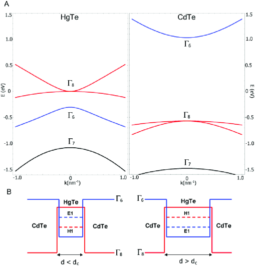
Figure 1: (A) Bulk energy bands of HgTe and CdTe near the $\Gamma$ point. (B) The CdTe/HgTe/CdTe quantum well in the normal regime $E1>H1$ with $d<d_{c}$ and in the inverted regime $H1>E1$ with $d>d_{c}$. In this, and all subsequent figures $\Gamma_{8}$/H1 ($\Gamma_{6}$/E1) symmetry is correlated with the color red (blue).

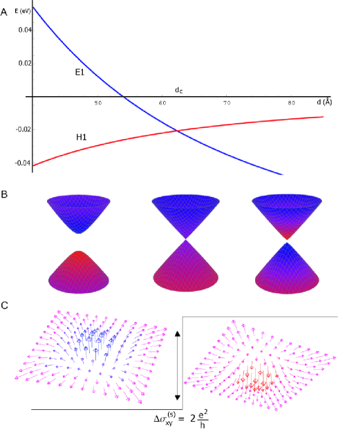
Figure 2: (A) Energy (eV) of $E1$ (blue) and $H1$ (red) bands at $k_{\parallel}=0$ vs. quantum-well thickness $d$ ($\AA$). (B) Energy dispersion relations $E(k_{x},k_{y})$ of the $E1,H1$ subbands at $40\AA,$ $63.5\AA$ and $70\AA$ from left to right. Colored shading indicates the symmetry type of band at that $k$-point. Places where the cones are more red (blue) indicates that the dominant states are H1 (E1) states at that point. Purple shading is a region where the states are more evenly mixed. For $40\AA$ the lower (upper) band is dominantly H1(E1). At $63.5\AA$ the bands are evenly mixed near the band crossing and retain their $d<d_{c}$ behavior moving further out in $k$-space. At $d=70\AA$ the regions near $k_{\parallel}=0$ have flipped their character but eventually revert back to the $d<d_{c}$ further out in $k$-space. Only this dispersion shows the meron structure (red and blue in the same band). (C) Schematic meron configurations representing the $d_{i}(k)$ vector near the $\Gamma$ point. The shading of the merons has the same meaning as the dispersion relations above. The change in meron number across the transition is exactly equal to $1$, leading to a quantum jump of the spin Hall conductance $\Delta\sigma_{xy}^{(s)}=2e^{2}/h.$ We measure all Hall conductances in electrical units. All of these plots are for Hg_0.32Cd_0.68Te/HgTe quantum wells.

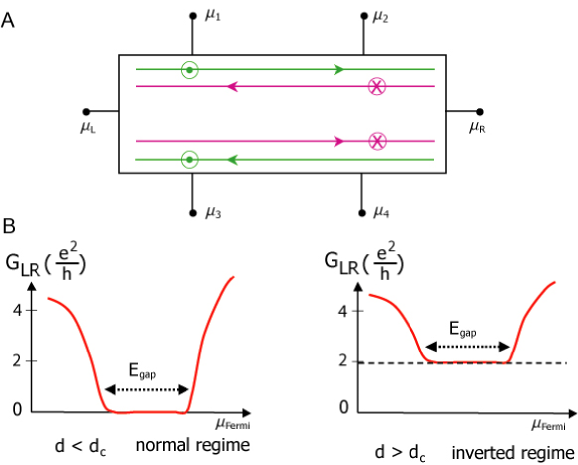
Figure 3: (A) Experimental setup on a six terminal Hall bar showing pairs of edge states with spin up (down) states green (purple). (B)A two-terminal measurement on a Hall bar would give $G_{LR}$ close to $2e^{2}/h$ contact conductance on the QSH side of the transition and zero on the insulating side. In a six-terminal measurement, the longitudinal voltage drops $\mu_{2}-\mu_{1}$ and $\mu_{4}-\mu_{3}$ vanish on the QSH side with a power law as the zero temperature limit is approached. The spin-Hall conductance $\sigma_{xy}^{(s)}$ has a plateau with the value close to $2\frac{e^{2}}{h}.$

2 Supporting Online Material

We show that our effective Hamiltonian can be derived perturbatively with $\textbf{k}\cdot\textbf{P}$ theory and is a quantitatively accurate description of the band structure for the $E1$ and the $H1$ subband states. We start from the $6$-band bulk Kane model which incorporates the $\Gamma_{6}$ and $\Gamma_{8}$ bands but neglects the split-off $\Gamma_{7}$ band( the contribution of the split-off band to the E1,H1 energies is less than $5\%$(S2)):

$${\cal{H}}(\vec{k})=\left(\matrix{E_{c}I_{2\times 2}+H_{c}&T_{2\times 4}\cr T^{\dagger}_{4\times 2}&E_{v}I_{4\times 4}+H_{v}\\ }\right)$$ (6)

where $E_{c}$ is the conduction band offset energy, $E_{v}$ is the valence band offset energy, $H_{c},H_{v}$ are the conduction and valence (Luttinger) band Hamiltonians, while $T(k)$ is the interaction matrix between the conduction and valence bands:

$$H_{c}=\left(\matrix{\frac{\hbar^{2}k^{2}}{2m^{\star}}&0\cr 0&\frac{\hbar^{2}k^{2}}{2m^{\star}}\cr}\right);\;\;T^{\dagger}=\left(\matrix{-\frac{1}{\sqrt{2}}Pk_{-}&0\cr\sqrt{\frac{2}{3}}Pk_{z}&-\frac{1}{\sqrt{6}}Pk_{-}\cr\frac{1}{\sqrt{6}}Pk_{-}&\sqrt{\frac{2}{3}}Pk_{z}\cr 0&\frac{1}{\sqrt{2}}Pk_{-}\cr}\right)$$

$$H_{v}=-\frac{\hbar^{2}}{2m_{0}}(\gamma_{1}+\frac{5}{2}\gamma_{2})k^{2}+\frac{\hbar^{2}}{m_{0}}\gamma_{2}(\vec{k}\cdot\vec{S})^{2}$$ (7)

where $m^{\star}$ is the effective electron mass in the conduction band, $k_{\pm}=k_{x}\pm ik_{y}$, $P=-\frac{\hbar}{m_{0}}\langle s|p_{x}|X\rangle$ is the Kane matrix element between the $s$ and $p$ bands with $m_{0}$ the bare electron mass, $\vec{S}$ is the spin-$3/2$ operator whose representation are the $4\times 4$ spin matrices, and $\gamma_{1},\gamma_{2}$ are the effective Luttinger parameters in the valence band. The ordered basis for this form of the Kane model is $(|\Gamma^{6},+1/2>,|\Gamma^{6},-1/2>,|\Gamma^{8},+3/2>,|\Gamma^{8},+1/2>,|\Gamma^{8},-1/2>,|\Gamma^{8},-3/2>).$ Although due to space constraints the above Hamiltonian is written in the spherical approximation, our calculations include the anisotropy effects generated by a third Luttinger parameter $\gamma_{3}\neq\gamma_{2}$. The quantum well growth direction is along $z$ with Hg_1-xCd_xTe for $z<-d/2$, HgTe for $-d/2<z<d/2$ and Hg_1-xCd_xTe for $z>d/2$. Our problem reduces to solving, in the presence of continuous boundary conditions, the Hamiltonian Eq. 6 in each of the $3$ regions of the quantum well. The material parameters $E_{c},E_{v},\gamma_{1,2,3}$, and $m^{\star}$, are discontinuous at the boundaries of the $3$ regions, taking the Hg_1-xCd_xTe/HgTe/Hg_1-xCd_xTe values (see Ref. (S1) for numerical values), so we have a set of $3$ multi-component eigenvalue equations coupled by the boundary conditions. The in-plane momentum is a good quantum number and the solution in each region takes the general form:

$${\cal{H}}(\vec{k})\psi(k_{x},k_{y},z)={\cal{H}}(k_{x},k_{y},-i\partial_{z})\psi(k_{x},k_{y},z);$$

$$\psi(k_{x},k_{y},z)=e^{i(k_{x}x+k_{y}y)}\Psi(z)$$ (8)

where $\Psi(z)$ is the envelope function spinor in the six component basis introduced earlier.

We solve the Hamiltonian analytically by first solving for the eigenstates at zero in-plane momentum, and then perturbatively finding the form of the Hamiltonian for finite in-plane k: ${\cal{H}}(k_{x},k_{y},-i\partial_{z})={\cal{H}}(0,0,-i\partial_{z})+\delta{\cal{H}}(k_{x},k_{y},-i\partial_{z})$. At $k_{x}=k_{y}=0$ we have the following Hamiltonian:

$${\cal{H}}(0,0,-i\partial_{z})=\left(\matrix{T&0&0&\sqrt{\frac{2}{3}}P(-i\partial_{z})&0&0\cr 0&T&0&0&\sqrt{\frac{2}{3}}P(-i\partial_{z})&0\cr 0&0&U+V&0&0&0\cr\sqrt{\frac{2}{3}}P(-i\partial_{z})&0&0&U-V&0&0\cr 0&\sqrt{\frac{2}{3}}P(-i\partial_{z})&0&0&U-V&0\cr 0&0&0&0&0&U+V}\right)$$ (9)

where $T=E_{c}(z)+(-\partial_{z}A(z)\partial_{z})$, $U=E_{v}(z)-(-\partial_{z}\gamma_{1}(z)\partial_{z})$, $V=2(-\partial_{z}\gamma_{2}(z)\partial_{z}).$ These parameters are treated as step functions in the $z$-direction with an abrupt change from the barrier region to the well region.

A general state in the envelope function approximation can be written in the following form:

$$\Psi(k_{x},k_{y},z)=e^{i(k_{x}x+k_{y}y)}\left(\matrix{f_{1}(z)\cr f_{2}(z)\cr f_{3}(z)\cr f_{4}(z)\cr f_{5}(z)\cr f_{6}(z)}\right).$$ (10)

At $k_{x}=k_{y}=0$ the $f_{3}$ and $f_{6}$ components decouple and form the spin up and down ($\pm$) states of the $H1$ subband. The $f_{1},f_{2},f_{4},f_{5}$ components combine together to form the spin up and down ($\pm$) states of the E1 and L1 subbands. The linear-in-$k_{z}$ operator $\sqrt{\frac{2}{3}}Pk_{z},$ in ${\cal{H}}(0,0,-i\partial_{z})$ forces the $|\Gamma_{6},\pm\frac{1}{2}\rangle(z)$ and $|\Gamma_{8},\pm\frac{1}{2}\rangle(z)$ components of the $E1$ band to have different reflection symmetry under $z\leftrightarrow-z$. The $|\Gamma_{6}\rangle$ band is symmetric in $z$ (exponentially decaying in CdTe and a $\cosh(z)$ dependence in HgTe) while the $|\Gamma_{8},m_{J}=\pm 1/2\rangle$ band is antisymmetric in $z$ (exponentially decaying in CdTe and a $\sinh(z)$ dependence in HgTe). The opposite choice of symmetry under $z\rightarrow-z$ reflection leads to the $L1$ band. However, this band is far away in energy from both the $E1$ and the $H1$ bands, does not cross either of them in the region of interest(S2), and we hence discard it.

For the E1 band we take the ansatz, already knowing it must be an interface state(S2), to be:

$$\Psi_{I}=\left(\matrix{e^{\alpha z}C_{1}\cr 0\cr\ 0\cr e^{\alpha z}C_{4}\cr 0\cr 0}\right), \Psi_{II}=\left(\matrix{(e^{\delta z}+e^{-\delta z})V_{1}\cr 0\cr 0\cr(e^{\delta z}-e^{-\delta z})V_{4}\cr 0\cr 0}\right), \Psi_{III}=\left(\matrix{e^{-\alpha z}C_{1}\cr 0\cr 0\cr-e^{-\alpha z}C_{4}\cr 0\cr 0}\right).$$ (11)

If we act on this ansatz with the Hamiltonian we decouple the $6\times 6$ matrix into two, coupled, one-dimensional Schrodinger equations:

$$Tf_{1}(z)+\sqrt{\frac{2}{3}}P(z)(-i\partial_{z})f_{4}(z)=Ef_{1}(z)$$ (12)

$$\sqrt{\frac{2}{3}}P(z)(-i\partial_{z})f_{1}(z)+(U-V)f_{4}(z)=Ef_{4}(z)$$ (13)

where $P,T,U,V$ are given above. Using the restrictions from the Hamiltonian, the continuity of each wavefunction component at the boundaries, and the continuity of the probability current across the boundary, we derive the following set of equations that determine $\alpha$ and $\delta$ as a function of E:

$$\frac{E_{c}^{(Cd)}-A^{(Cd)}\alpha^{2}(E)-E}{\sqrt{\frac{2}{3}}\frac{P}{i}\alpha(E)}=\frac{\sqrt{\frac{2}{3}}\frac{P}{i}\alpha(E)}{E_{v}^{(Cd)}+(\gamma_{1}^{(Cd)}+2\gamma_{2}^{(Cd)})\alpha^{2}(E)-E}$$ (14)

$$\frac{E_{c}^{(Hg)}-A^{(Hg)}\delta^{2}(E)-E}{\sqrt{\frac{2}{3}}\frac{P}{i}\delta(E)}=\frac{\sqrt{\frac{2}{3}}\frac{P}{i}\delta(E)}{E_{v}^{(Hg)}+(\gamma_{1}^{(Hg)}+2\gamma_{2}^{(Hg)})\delta^{2}(E)-E}$$ (15)

where a parameter $X^{(Cd)}$ means the value of that parameter in the CdTe barrier material and $X^{(Hg)}$ is the value in the HgTe well material. Once we have $\alpha(E)$ and $\delta(E)$ we can use them to determine $E$ through the following equation derived from the boundary conditions:

$$\frac{E_{c}^{(Cd)}-A^{(Cd)}\alpha^{2}(E)-E}{\alpha(E)}=-\tanh\left(\frac{\delta(E)d}{2}\right)\left(\frac{E_{c}^{(Hg)}-A^{(Hg)}\delta^{2}(E)-E}{\delta(E)}\right).$$ (16)

These rational transcendental equations are solved numerically to obtain the energy of the $E1$ subband at $k_{x}=k_{y}=0.$

We can follow a similar procedure to derive the energy of the $H1$ subband. The heavy hole subband (at $k_{x}=k_{y}=0$) completely decouples from the other bands and we have the one-dimensional, one-component Hamiltonian:

$$Hf_{3}(z)=E_{v}(z)-(\gamma_{1}(z)-2\gamma_{2}(z))(-\partial_{z}^{2})f_{3}(z)=Ef_{3}(z).$$ (17)

We have the wavefunction in three regions

$$\left(\matrix{\Psi_{I}(z)\cr\Psi_{II}(z)\cr\Psi_{III}(z)}\right)=\left(\matrix{C_{3}e^{\beta z}\cr V_{3}\cos(\kappa z)\cr C_{3}e^{-\beta z}}\right)$$ (18)

where $\beta^{2}(E)=\frac{E-E_{v}^{(Cd)}}{\gamma_{1}^{(Cd)}-2\gamma_{2}^{(Cd)}}$ and $\kappa^{2}(E)=\frac{E_{v}^{(Hg)}-E}{\gamma_{1}^{(Hg)}-2\gamma_{2}^{(Hg)}}.$ We can pick $C_{3}=1$ which gives us the relation

$$V_{3}=\frac{e^{-\frac{1}{2}\beta d}}{\cos(\kappa(E)d/2)}$$ (19)

from the boundary condition at $z=-d/2.$ Finally, we need to normalize the wavefunction to get the coefficients. The energy of this state is determined by considering the conservation of probability current across the boundary. The following equation is solved for the energy:

$$\frac{1}{(\gamma_{1}^{(Cd)}-2\gamma_{2}^{(Cd)})\beta(E)}=\frac{1}{(\gamma_{1}^{(Hg)}-2\gamma_{2}^{(Hg)})\kappa(E)}\cot(\kappa(E)d/2).$$ (20)

We repeat both of these processes on a state with only $f_{2}(z)$ and $f_{5}(z)$ non-zero and on a state with only $f_{6}(z)$ non-zero and to get the $E1^{-}$ and $H1^{-}$ bands respectively. We have the forms of these states at $k_{x}=k_{y}=0$ and can use $k\cdot P$ perturbation theory to derive a two dimensional Hamiltonian near the $\Gamma$ point in $k$-space.

3 Perturbation Theory and Effective Hamiltonian

Define an ordered set of basis vectors $(|E1,+>,|H1,+>,|E1,->,|H1,->).$ We can write the effective Hamiltonian as:

$$H_{ij}(k_{x},k_{y})=\int_{-\infty}^{\infty}dz<\psi_{j}|H_{6\times 6}(k_{x},k_{y},-i\partial_{z})|\psi_{i}>$$ (21)

where $\psi_{i}$ is the $i$-th element of the basis set given above which will give a $4\times 4$ effective Hamiltonian. The integrals must be split into the three regions defined above, and the parameters from each material must be accounted for in the Hamiltonian. This Hamiltonian depends on the quantum-well width $d,$ and once $d$ is specified we can numerically calculate the matrix-elements. It is important to note that $f_{1}(z),f_{2}(z),f_{3}(z),f_{6}(z)$ are symmetric with respect to $z$ and $f_{4}(z),f_{5}(z)$ are antisymmetric in $z$(S2) which is a useful simplification in performing the integrals. An example of one integral is of the form:

$$\int dzf_{3}^{*}(z)\left\{\gamma_{3}(z),-i\partial_{z}\right\}f_{4}(z)=$$

$$\int dz\frac{1}{i}\left(2\gamma_{3}(z)f_{3}^{*}(z)\partial_{z}f_{4}(z)+f_{3}^{*}(z)f_{4}(z)\partial_{z}\gamma_{3}(z)\right).$$ (22)

The functional form of $\gamma_{3}(z)$ is

$$\gamma_{3}(z)=\gamma_{3}^{(Cd)}(\theta(-d/2-z)+\theta(z-d/2))+\gamma_{3}^{(Hg)}(\theta(z+d/2)-\theta(z-d/2)).$$ (23)

The $z$-derivative acting on this function produces $\delta$-function terms that contribute a term proportional to $(\gamma_{3}^{(Cd)}-\gamma_{3}^{(Hg)})$ to the integral which vanish when these material parameters are equal. The integral then has to be evaluated numerically.

After calculating the matrix-elements we are left with an effective Hamiltonian parameterized in the following way:

$${\cal{H}}(k_{x},k_{y})=\left(\matrix{\epsilon_{k}+{\cal{M}}(k)&Ak_{-}&0&0\cr Ak_{+}&\epsilon_{k}-{\cal{M}}(k)&0&0\cr 0&0&\epsilon_{k}+{\cal{M}}(k)&-Ak_{+}\cr 0&0&-Ak_{-}&\epsilon_{k}-{\cal{M}}(k)}\right)$$ (24)

where $\epsilon_{k}=C-D(k_{x}^{2}+k_{y}^{2}),$ ${\cal{M}}(k)=M-B(k_{x}^{2}+k_{y}^{2}),$ $k_{\pm}=k_{x}\pm ik_{y},$ and $A,B,C,D,M$ depend on the specified quantum-well width. For values of these parameters at $d=40\AA$ and $d=70\AA$ see Table 1. This Hamiltonian is block diagonal and can be written in the form

$${\cal{H}}(k_{x},k_{y})=\left(\matrix{H(k)&0\cr 0&H^{\ast}(-k)}\right)$$ (25)

where $H(k)=\epsilon_{k}I_{2\times 2}+d^{a}(k)\sigma^{a},$ with $d^{1}=Ak_{x},d_{2}=Ak_{y},$ and $d^{3}={\cal{M}}(k)=M-B(k_{x}^{2}+k_{y}^{2}).$ Finally, we define a unitary transformation:

$$U=\left(\matrix{I_{2\times 2}&0\cr 0&-\sigma^{z}}\right)$$ (26)

and take $U^{\dagger}H_{4\times 4}U$ which reverses the sign of the linear $k$ terms in the lower block and puts it ${\cal{H}}$ into the form

$${\cal{H}}(k_{x},k_{y})=\left(\matrix{H(k)&0\cr 0&H^{\ast}(k)}\right).$$ (27)

$U$ does not affect the $z$-direction of spin and simply rotates the $x$ and $y$ axes in the lower block of the Hamiltonian by $\pi.$ The energy dispersions for these bands are given in Fig. 1 of the supporting online material for several values of $d.$

$d$ ($\AA$)	$A(eV)$	$B(eV)$	$C(eV)$	$D(eV)$	$M(eV)$
58	-3.62	-18.0	-0.0180	-0.594	0.00922
70	-3.42	-16.9	-0.0263	0.514	-0.00686

Table 1: Parameters for Hg_0.32Cd_0.68Te/HgTe quantum wells.

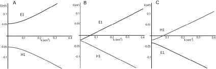
Figure 4: Dispersion relations for the $E1$ and $H1$ subbands for(A) $d=40\AA$ (B) $d=63.5\AA$ (C) $d=70\AA.$

Supporting References and Notes

• E.G. Novik et. al., Phys. Rev. B 72, 035321 (2005).

• A. Pfeuffer-Jeschke, Ph.D. Thesis, University of Wurzburg, Germany, 2000.

References and Notes

- 1. M.I. D’yakonov, V.I. Perel, Phys. Lett. A 35, 459 (1971).
- 2. S. Murakami, N. Nagaosa, S.C. Zhang, Science 301, 1348 (2003).
- 3. J. Sinova et. al., Phys. Rev. Lett. 92, 126603 (2004).
- 4. Y. Kato et. al., Science 306, 1910 (2004).
- 5. J. Wunderlich, B. Kaestner, J. Sinova, T. Jungwirth, Phys. Rev. Lett. 94, 47204 (2005).
- 6. S. Murakami, N. Nagaosa, S.C. Zhang, Phys. Rev. Lett. 93, 156804 (2004).
- 7. C. L. Kane, E. J. Mele, Phys. Rev. Lett. 95, 226801 (2005).
- 8. B.A. Bernevig, S.C. Zhang, Phys. Rev. Lett. 96, 106802 (2006).
- 9. X.L. Qi, Y.S. Wu, S.C. Zhang, Phys. Rev. B 74, 085308 (2006).
- 10. C. L. Kane, E. J. Mele, Phys. Rev. Lett. 95, 146802 (2005).
- 11. C. Wu, B.A. Bernevig, S.C. Zhang, Phys. Rev. Lett. 96, 106401 (2006).
- 12. C. Xu, J. Moore, Phys. Rev. B 73, 045322 (2006).
- 13. L. Sheng et. al., Phys. Rev. Lett. 65, 136602 (2005).
- 14. M. Onoda, Y. Avishai, N. Nagaosa, cond-mat/0605510.
- 15. D.J. Thouless, M. Kohmoto, M.P. Nightingale, M. den Nijs, Phys. Rev. Lett. 49, 405 (1982).
- 16. Y. Yao, F. Ye, X.L. Qi, S.C. Zhang, Z. Fang, cond-mat/0606350.
- 17. H. Min, et al., Phys. Rev. B 74, 165310 (2006).
- 18. S. Murakami, cond-mat/0607001.
- 19. E.O. Kane, J. Phys. Chem. Solids 1, 249 (1957).
- 20. E.G. Novik et. al., Phys. Rev. B 72, 035321 (2005).
- 21. A. Pfeuffer-Jeschke, Ph.D. Thesis, University of Wurzburg, Germany, 2000.
- 22. A. N. Redlich, Phys. Rev. D 29, 2366 (1984).
- 23. H. B. Nielsen, M. Ninomiya, Nucl. Phys. B 185, 20 (1981).
- 24. X.L. Qi, Y.S. Wu, S.C. Zhang, Phys. Rev. B 74, 045125 (2006).
- 25. M. F. L. Goleterman, K. Jansen, D.B. Kaplan, Phys. Lett. B 301, 219 (1993).
- 26. F.D.M. Haldane, Phys. Rev. Lett. 60, 635 (1988).
- 27. K. Ortner et. al., Applied Physics Letters 79, 3980 (2000).
- 28. C. R. Becker, V. Latussek, A. Pfeuffer-Jeschke, G. Landwehr, L. W. Molenkamp, Phys. Rev. B 62, 10353 (2000).
-
1.