Soft elasticity in biaxial smectic and smectic-$C$ elastomers

Abstract

Ideal (monodomain) smectic-$A$ elastomers crosslinked in the smectic-$A$ phase are simply uniaxial rubbers, provided deformations are small. From these materials smectic-$C$ elastomers are produced by a cooling through the smectic-$A$ to smectic-$C$ phase transition. At least in principle, biaxial smectic elastomers could also be produced via cooling from the smectic-$A$ to a biaxial smectic phase. These phase transitions, respectively from $D_{\infty h}$ to $C_{2h}$ and from $D_{\infty h}$ to $D_{2h}$ symmetry, spontaneously break the rotational symmetry in the smectic planes. We study the above transitions and the elasticity of the smectic-$C$ and biaxial phases in three different but related models: Landau-like phenomenological models as functions of the Cauchy–Saint-Laurent strain tensor for both the biaxial and the smectic-$C$ phases and a detailed model, including contributions from the elastic network, smectic layer compression, and smectic-$C$ tilt for the smectic-$C$ phase as a function of both strain and the $c$-director. We show that the emergent phases exhibit soft elasticity characterized by the vanishing of certain elastic moduli. We analyze in some detail the role of spontaneous symmetry breaking as the origin of soft elasticity and we discuss different manifestations of softness like the absence of restoring forces under certain shears and extensional strains.

I Introduction

Liquid crystalline elastomers WarnerTer2003 are fascinating hybrid materials that combine the elastic properties of rubber with the orientational and positional order of liquid crystals deGennesProst93_Chandrasekhar92 . As in conventional liquid crystals, there exists a great variety of phases in liquid crystalline elastomers. For example, nematic, cholesteric, smectic-$A$ (Sm$A$), chiral smectic-$A^{*}$ (Sm$A^{\ast}$), smectic-$C$ (Sm$C$), and chiral smectic-$C^{\ast}$ (Sm$C^{\ast}$) phases have been created in elastomeric forms WarnerTer2003 . Among these elastomers, nematics have to date received the most attention leading to the discovery of a number of remarkable properties of these materials such as soft elasticity golubovic_lubensky_89 ; FinKun97 ; VerWar96 ; War99 ; LubenskyXin2002 , dynamic soft elasticity terentjev&Co_NEhydrodyn ; stenull_lubensky_2004 ; stenull_lubensky_comment , and anomalous elasticity stenull_lubensky_epl2003 ; Xing_Radz_03 ; stenull_lubensky_anomalousNE_2003 . In contrast, the understanding of smectic elastomers is much less developed, at least from a theoretical point of view. Given that there is a substantial literature treating the synthesis and experimental properties of smectic elastomers shibaev_81_82 ; fischer_95 ; bremer&Co_1993 ; benne&Co_1994 ; hiraoka&CO_2001 ; hiraoka&CO_2005 ; GebhardZen1998 ; ZentelBre2000 ; StannariusZen2002 , that smectic elastomers have intriguing properties and potential for device applications such as manometer-scale actuators lehmann&Co_01 , and that smectics play a leading role in conventional liquid crystals where they have attracted outstanding scientific and technological interest since the discovery of spontaneous ferroelectricity in $C^{\ast}$ smectics meyer&Co_75 , it is clear that a deeper theoretical understanding of smectic elastomers is desirable.

To date there have been, as far as we know, only relatively few theoretical investigations of smectic elastomers for the apparent reason that such investigations are difficult due to the complexity and low symmetry of the material. Terentjev and Warner developed expressions for the elastic energies of Sm$A$ and Sm$A^{\ast}$ elastomers terentjev_warner_SmA_1994 as well as for Sm$C$ and Sm$C^{\ast}$ elastomers terentjev_warner_SmC_1994 based on group theoretical arguments. The coupling of the smectic layers to the elastic network was critically discussed and shortcomings of Ref. terentjev_warner_SmA_1994 in this respect were corrected in lubensky&Co_94 . Subsequently, the damping effect of the rubber-elastic matrix on the fluctuations of the smectic layers, leading to a suppression of the Landau-Peierls instability and true one-dimensional long-range order, was analyzed in terentjev_warner_lubensky_95 . Weilepp and Brand weilepp_brand_1998 discussed an undulation instability as a possible explanation for the turbidity of Sm$A$ elastomers under stretch along the normal of the smectic layers. Osborne and Terentjev osborne_terentjev_2000 derived expressions for the effective elastic constants of Sm$A$ elastomers when these are viewed as effectively uniaxial systems and revisited the suppression of fluctuations of the smectic layers. Very recently, Adams and Warner (AW) adams_warner_2005 ; adams_warner_SmC_2005 ; adams_warner_2006 set up a model for the elasticity of smectic elastomers by extending the so-called neoclassic model of rubber elasticity, which was originally developed and very successfully used to describe nematic elastomers WarnerTer2003 , to include the effects of smectic layering. Also just recently we worked out theories for the low-frequency long-wavelength dynamics of smectic elastomers in respectively the Sm$A$, biaxial and Sm$C$ phases stenull_lubensky_SmCdynamics .

In principle, smectic elastomers can be produced either by cooling nematic elastomers through the transition to the smectic phase or by crosslinking in the smectic phase. Both Sm$A$ and Sm$C$ elastomers have been prepared mostly by the second method, e.g., by crosslinking side chain liquid crystalline polymers, which have a tendency to form layers because their mesogens are often immiscible with the polymeric backbone shibaev_81_82 , or by crosslinking polymer chains or hydrophobic tails in bilayer lamellar phases of respectively diblock copolymers or surfactant molecules fischer_95 . Crosslinking in the smectic phase tends to lock the smectic layers to the crosslinked network lubensky&Co_94 . Without this lock-in, the phase of the smectic mass-density-wave can translate freely relative to the elastomer as it can in smectics in aerogels radzihovsky_toner_99 . To keep our discussion as simple as possible, we will not consider in the following the case of crosslinking in the nematic phase, and we take the lock-in of the smectic layers and the elastic matrix as given.

As in nematics, unconventional properties are most pronounced in samples of smectic elastomers that have an ideal, monodomain morphology so that the director has a uniform orientation throughout. In practice, however, liquid crystal elastomers tend to be non-ideal, i.e. the material segregates into many domains, each having its own local director. In order to avoid such polydomain samples, elaborate crosslinking schemes involving electric or mechanical external fields for aligning the director have been developed and successfully applied to smectic elastomers bremer&Co_1993 ; benne&Co_1994 ; hiraoka&CO_2001 . The latest achievement in this respect was reported very recently by Hiraoka et al. hiraoka&CO_2005 , who produced a monodomain sample of a Sm$C$ elastomer forming spontaneously from a Sm$A$ phase upon cooling and carried out experiments demonstrating its spontaneous and reversible deformation in a heating an cooling process.

A monodomain Sm$A$ elastomer crosslinked in the Sm$A$ phase is effectively a uniaxial solid with $D_{\infty h}$ symmetry, at least for small deformations. For lager deformations, however, Sm$A$ elastomers can show unconventional effects, as do Sm$A^{\ast}$ elastomers in external electric fields. These unconventional effects in Sm$A$ elastomers are outside the scope of this paper and will be addressed in a separate paper stenull_lubensky_smA_2006 .

The elastic properties of a Sm$C$ elastomer depend on whether it was crosslinked in the Sm$A$ or Sm$C$ phase. If it is prepared by crosslinking in a Sm$C$ phase, reached either by stretching or by applying an external electric field, it is a conventional biaxial solid with $C_{2h}$ symmetry. If, however, the Sm$C$ phase develops spontaneously upon cooling from a uniaxial Sm$A$ (as in the work of Hiraoka et al.) then the underlying phase transition from $D_{\infty h}$ to $C_{2h}$ symmetry (see Fig. 1) spontaneously breaks the continuous rotational symmetry in the smectic planes. As a consequence of the Goldstone theorem that requires any phase with a spontaneously broken continuous symmetry to have modes whose energy vanishes with wavenumber, like monodomain nematic elastomers golubovic_lubensky_89 ; FinKun97 ; VerWar96 ; War99 ; LubenskyXin2002 , these Sm$C$ elastomers are predicted to exhibit soft elasticity characterized by the vanishing of a certain elastic modulus and the associated absence of restoring forces to strains along specific symmetry directions stenull_lubensky_letter_2005 .

Figure 1: Sample distortion and rotations of the Frank director $\bm{{\rm n}}$, the uniaxial anisotropy axis $\bm{{\rm e}}\equiv\bm{{\rm e}}_{z}$, and the layer normal $\bm{{\rm N}}$ in a transition from a (a) Sm$A$ to (b) a biaxial and (c) a sheared Sm$C$ elastomer. In part (c) we chose the geometry, i.e., the coordinate system in target space, so that the smectic layers do not rotate.

Though biaxial phases are notoriously hard to find in nature, it is possible, at least in principle, that a biaxial Sm$A$ phase spontaneously forms upon cooling from a Sm$A$ elastomer. In what follows, we will often simply refer to biaxial Sm$A$ elastomers as biaxial smectic elastomers or biaxial elastomers. In contrast to the aforementioned phase transition to a soft Sm$C$ elastomer, the transition to the biaxial Sm$A$ phase involves no net tilt of the mesogens and takes the system to $D_{2h}$ instead of $C_{2h}$ symmetry (see Fig. 1). Nontheless, this transition also breaks the rotational invariance in the smectic layers spontaneously and thus the emerging biaxial phase is soft stenull_lubensky_letter_2005 similar to ideal nematic and Sm$C$ elastomers.

In this paper we study the phase transitions from Sm$A$ elastomers to biaxial and Sm$C$ elastomers and the elasticity of the emergent phases. As briefly presented in Ref. stenull_lubensky_letter_2005 , we set up three different but related models. Our first two models involve only elastic degrees of freedom, i.e., they involve exclusively the usual strain tensor. Our third model also includes the Frank director specifying the direction of local molecular order. Each of the models is analyzed within mean-field theory, revealing as the primary result the soft elasticity of biaxial and Sm$C$ elastomers stenull_lubensky_letter_2005 ; adams_warner_SmC_2005 ; adams_warner_2006 alluded to in the forgoing paragraphs.

The outline of our paper is as follows: Section II briefly reviews the Lagrange formulation of elasticity theory in the context of uniaxial elastomers to establish notation and to provide a starting point for our models to follow. Section III presents our strain-only theory for biaxial elastomers. We study the transition from the Sm$A$ to the biaxial state and the elastic properties of the latter. We derive the elastic energy density of the biaxial state and discuss its softness with respect to certain shears and extensional strains. Section IV contains our strain-only theory for Sm$C$ elastomers. We investigate the Sm$A$-to-Sm$C$ transition and calculate the elastic energy density of the Sm$C$ phase. Different manifestations of the softness of Sm$C$ elastomers are pointed out. Section V formulates our theory for Sm$C$ elastomers with strain, Frank director, and smectic layers. Using the polar decomposition theorem, we derive transformations between vectors that transform according to operations on reference-space positions $\bm{{\rm x}}$ of the undistorted medium and those that transform according to operations on target-space positions $\bm{{\rm R}}(\bm{{\rm x}})$ of the distorted medium, and we formulate the elastic energy for coupled director and strain in terms of nonlinear-strain and director fields that transform under reference-state operations only. In this approach, phase transitions can be studied without specifying actual orientation in space. We develop a full model free energy that includes contributions from the crosslinked network, smectic layer compression, and coupling between the Frank director and the smectic layer normal. Then, as above, we study the phase transition from the Sm$A$ to the Sm$C$ phase and the elastic energy density of the emergent phase. In addition, we discuss the general form of soft deformations and strains in Sm$C$ elastomers based on rotational invariance in the smectic planes and we elaborate on softness under extensional strains. Concluding remarks are given in Sec. VI. There are in total 4 appendixes which contain technical details or arguments that lie somewhat aside the line of thought of the main text.

II Lagrangian description of uniaxial elastomers

As argued above, ideal Sm$A$ elastomers are macroscopically simply uniaxial rubbers, but with nonlinear properties that distinguish them from simple uniaxial solids. We will employ the usual Langrangian formalism Landau-elas ; tomsBook of elasticity theory. Here, we briefly review key elements of this formalism in the context of uniaxial elastomers to establish notation and to provide some background information.

In the Langrangian formalism mass points in an undistorted medium (or body), which we take as the reference space, are labelled by vectors $\bm{{\rm x}}$. Mass points of the distorted medium are at positions

$$\bm{{\rm R}}(\bm{{\rm x}})=\bm{{\rm x}}+\bm{{\rm u}}(\bm{{\rm x}}),$$ (1)

that constitute what we call the target space. Both reference space points $\bm{{\rm x}}$ and target space points $\bm{{\rm R}}(\bm{{\rm x}})$ exist in the same physical Euclidean space $\cal E$ where measurements are made. Thus, $\bm{{\rm R}}(\bm{{\rm x}})$ is a mapping from $\cal E$ to $\cal E$. Both $\bm{{\rm x}}$ and $\bm{{\rm R}}(\bm{{\rm x}})$ can be decomposed into components along the standard orthonormal basis $\{\bm{{\rm a}}_{i}|i=x,y,z\}$ of $\cal E$:

$$\bm{{\rm x}}=x_{i}\,\bm{{\rm a}}_{i},\qquad\bm{{\rm R}}(\bm{{\rm x}})=R_{i}(\bm{{\rm x}})\,\bm{{\rm a}}_{i}.$$ (2)

Here and in what follows, we use the summation convention on repeated indices unless we indicate otherwise. We will also use the convention that indices from the middle of the alphabet run over all space coordinates, $i,j,k=x,y,z$. We choose our coordinate system so that the $z$-axis is along the uniaxial direction of the initial reference material. Indices from the beginning of the alphabet, $a$, $b$, $c$, run over $x$ and $y$ only, i.e., over directions perpendicular to the anisotropy axis.

Though reference- and target-space vectors both exist in $\cal E$, they transform under distinct and independent transformation operations. Let $\underline{\underline{O}}_{R}$ and $\underline{\underline{O}}_{T}$ denote, respectively, matrices describing transformations (which we will take mostly to be rotations but which could include reflections and inversions as well) in the reference and target spaces; then under these transformations, $\bm{{\rm x}}\rightarrow\bm{{\rm x}}^{\prime}=\underline{\underline{O}}_{R}\bm{{\rm x}}$ and $\bm{{\rm R}}(\bm{{\rm x}})\rightarrow\bm{{\rm R}}^{\prime}(\bm{{\rm x}})=\underline{\underline{O}}_{T}\bm{{\rm R}}(\bm{{\rm x}})$, or in terms of components relative to the $\bm{{\rm a}}$-basis

$$R^{\prime}_{i}(\bm{{\rm x}}) = O_{T,ij}R_{j}(\bm{{\rm x}})\,,$$ (3a)

$$x^{\prime}_{i} = O_{R,ij}\,x_{j}\,.$$ (3b)

Unless otherwise specified, we will view $\underline{\underline{O}}_{R}$ and $\underline{\underline{O}}_{T}$ as operators that rotate vectors rather than coordinate systems.

Elastic energies are invariant under arbitrary rigid rotations and translations in the target space and under symmetry operations of the references space of the form $\bm{{\rm x}}\rightarrow\bm{{\rm x}}^{\prime}=\underline{\underline{O}}_{R}^{-1}\bm{{\rm x}}+\bm{{\rm b}}$, where $\bm{{\rm b}}$ is a constant vector and $\underline{\underline{O}}_{R}$ is a matrix associated with some symmetry element of the reference space. Thus, elastic energies are invariant under transformations of the form

$$\bm{{\rm R}}(\bm{{\rm x}})\rightarrow\bm{{\rm R}}^{\prime}(\bm{{\rm x}}^{\prime})=\underline{\underline{O}}_{T}\bm{{\rm R}}(\underline{\underline{O}}_{R}^{-1}\bm{{\rm x}}+\bm{{\rm b}})+{\bm{{\rm X}}},$$ (4)

where $\underline{\underline{O}}_{T}$ is an arbitrary target-space rotation matrix and ${\bm{{\rm X}}}$ is a constant displacement vector. In what follows, we will generally ignore the displacements ${\bm{{\rm X}}}$ and $\bm{{\rm b}}$. The use of $\underline{\underline{O}}_{R}^{-1}$ in Eq. (4) rather than $\underline{\underline{O}}_{R}$ is a matter of convention footnoteRotationConnvention . With the choice $\underline{\underline{O}}_{R}^{-1}$, when $\underline{\underline{O}}_{T}=\underline{\underline{\delta}}$ where $\underline{\underline{\delta}}$ is the unit matrix, the mapping $\bm{{\rm R}}^{\prime}(\bm{{\rm x}})$ takes the point $\underline{\underline{O}}_{R}\bm{{\rm x}}$ to the same point in $\cal E$ as the mapping $\bm{{\rm R}}(\bm{{\rm x}})$ takes the point $\bm{{\rm x}}$.

We will usually represent the the reference-space points $\bm{{\rm x}}$ in terms of their coordinates relative to the basis $\{\bm{{\rm a}}_{i}\}$. We will, however, find it useful on occasion to consider orthonormal bases locked to the reference medium and to represent reference-space vectors relative to them. The initial basis $\{\tilde{\bm{{\rm e}}}_{i}|i=x,y,z\}$ is identical to the basis $\{\bm{{\rm a}}_{i}|i=x,y,z\}$, and $\bm{{\rm x}}=x_{i}\bm{{\rm a}}_{i}\equiv x_{i}\tilde{\bm{{\rm e}}}_{i}$. $\tilde{\bm{{\rm e}}}_{z}$ is thus a vector along the uniaxial axis of the undistorted body e-n0 . Under rotations of the body basis, $\bm{{\rm x}}=x^{\prime}_{i}\tilde{\bm{{\rm e}}}^{\prime}_{i}=x_{i}\bm{{\rm e}}_{i}$, where

$$\tilde{\bm{{\rm e}}}^{\prime}_{i}=O_{R,ij}\tilde{\bm{{\rm e}}}_{j}$$ (5)

and $x^{\prime}_{i}=O_{R,ij}x_{j}$. As we shall discuss in more detail in Sec. V.1 associated with each reference-space vector, there is a target-space vector of the same length. Thus, associated with the reference basis $\{\tilde{\bm{{\rm e}}}_{i}\}$, there is a target basis $\{\bm{{\rm e}}_{i}\}$. In particular there is a target-space anisotropy direction $\bm{{\rm e}}_{z}$ associated with $\tilde{\bm{{\rm e}}}_{z}$.

Distortions of the reference medium are described by the Cauchy deformation tensor $\underline{\underline{\Lambda}}$ with components

$$\Lambda_{ij}=\partial R_{i}/\partial x_{j}\equiv\partial_{j}R_{i}\,.$$ (6)

It transforms under the operations of Eq. (3) according to

$$\underline{\underline{\Lambda}}(\bm{{\rm x}})\rightarrow\underline{\underline{O}}_{T}\,\underline{\underline{\Lambda}}(\bm{{\rm x}}^{\prime})\,\underline{\underline{O}}_{R}^{-1}\,$$ (7)

i.e., the right subscript transforms under target-space rules and the left under reference-space rules. Usually, Lagrangian elastic energies are expressed in terms of the Cauchy-Saint-Venant Love1944 ; Landau-elas nonlinear strain tensor $\underline{\underline{u}}=(\underline{\underline{g}}-\underline{\underline{\delta}})/2$, where

$$\underline{\underline{g}}=\underline{\underline{\Lambda}}^{T}\underline{\underline{\Lambda}}$$ (8)

is the metric tensor. The components of $\underline{\underline{u}}$ are

$$u_{ij}(\bm{{\rm x}}) =\textstyle{\frac{1}{2}}\,(\Lambda^{T}_{ik}\Lambda_{kj}-\delta_{ij})$$ (9a)

$$=\textstyle{\frac{1}{2}}\,(\partial_{i}u_{j}+\partial_{j}u_{i}+\partial_{i}u_{k}\partial_{j}u_{k})\,.$$ (9b)

The strain $\underline{\underline{u}}$ is a reference-space tensor: it is invariant under transformations $\underline{\underline{O}}_{T}$ in the target space, but it transforms like a tensor under reference-space transformations:

$$\underline{\underline{u}}(\bm{{\rm x}})\rightarrow\underline{\underline{O}}_{R}\,\underline{\underline{u}}(\bm{{\rm x}}^{\prime})\,\underline{\underline{O}}_{R}^{-1}\,.$$ (10)

This expression applies both to physical transformations of reference-space vectors under $x^{\prime}_{i}=O_{R,ij}^{-1}x_{j}$ or under changes of basis described by Eq. (5) under which $\Lambda_{ij}\rightarrow\Lambda^{\prime}_{ij}=\partial R_{i}/\partial x^{\prime}_{j}=\Lambda_{ik}O_{R,kj}^{-1}$.

To discuss incompressible materials, such as most elastomers, it can be more appropriate to use variables other than the strain tensor to account for deformations that are not pure shear. In the case of uniaxial elastomers, such variables are the relative change of the system volume $V$,

$$\eta\equiv\delta V/V=[\det\underline{\underline{\Lambda}}^{T}\underline{\underline{\Lambda}}]^{1/2}-1=[(\det(1+2\underline{\underline{u}})]^{1/2}-1\,,$$ (11a)

and the relative change of separation of mass points whose separation vector in the reference state is along the $$z$$ axis:

$$\eta_{z}\equiv\delta L_{z}/L_{z}=|\Lambda_{iz}\Lambda_{iz}|^{1/2}-1=(1+2u_{zz})^{1/2}-1\,.$$ (11b)

Using these variables and, where appropriate, the elements of the strain tensor, the elastic free energy density of a uniaxial elastomer to harmonic order can be expressed as

$$f_{\text{uni}} =\textstyle{\frac{1}{2}}\,C_{1}\,\eta_{z}^{2}+C_{2}\,\eta_{z}\eta+\textstyle{\frac{1}{2}}\,C_{3}\,\eta^{2}$$

$$+C_{4}\,\hat{u}_{ab}^{2}+C_{5}\,u_{az}^{2},$$ (12)

where

$$\hat{u}_{ab}=u_{ab}-\ \textstyle{\frac{1}{2}}\,\delta_{ab}u_{cc}$$ (13)

is the two-dimensional symmetric, traceless strain tensor with two-independent components that can be expressed as $\underline{\underline{\hat{u}}}=u_{1}(\tilde{\bm{{\rm e}}}_{x}\tilde{\bm{{\rm e}}}_{x}-\tilde{\bm{{\rm e}}}_{y}\tilde{\bm{{\rm e}}}_{y})+u_{2}(\tilde{\bm{{\rm e}}}_{x}\tilde{\bm{{\rm e}}}_{y}+\tilde{\bm{{\rm e}}}_{y}\tilde{\bm{{\rm e}}}_{x})$. The elastic constant $C_{1}$ describes dilation or compression along $z$ and $C_{3}$ describes expansion or compression of the bulk volume. $C_{2}$ couples these two types of deformations. $C_{4}$ and $C_{5}$ respectively describe shears in the plane perpendicular to the anisotropy axis and in the planes containing it. With the variables used in Eq. (II) it is evident that the incompressible limit corresponds to $C_{3}\rightarrow\infty$.

If one approximates $\eta$ and $\eta_{z}$ by the respective leading terms in the strains one is left with

$$\eta =u_{ii}+O(u_{ij}^{2})\,,$$ (14a)

$$\eta_{z} =u_{zz}+O(u_{zz}^{2})\,.$$ (14b)

and the elastic energy density (II) reduces to the more standard-type expression

$$f_{\text{uni}} =\textstyle{\frac{1}{2}}\,C_{1}\,u_{zz}^{2}+C_{2}\,u_{zz}u_{ii}+\textstyle{\frac{1}{2}}\,C_{3}\,u_{ii}^{2}$$

$$+C_{4}\,\hat{u}_{ab}^{2}+C_{5}\,u_{az}^{2}.$$ (15)

Our models to be presented in the following are in spirit Landau expansions in powers of $u_{ij}$ or in powers of $u_{ij}$ and the Frank director, respectively. Hence, for our purposes, the approximations in Eqs. (14) will be sufficient, and we can use Eq. (II) as a starting point for the construction of our models. As we show in Appenix A, using Eq. (II), instead of the more general elastic energy density Eq. (II), leaves our results qualitatively unchanged, though the more general theory is needed for a correct description of the incompressible limit.

III Biaxial smectic-$A$ elastomers – strain-only theory

In our first theory we consider the case that the shear modulus $C_{4}$ becomes negative as it will in response to biaxial ordering of the constituent mesogens of a uniaxial Sm$A$ elastomer.

III.1 Phase transition from uniaxial to biaxial elastomers

If $C_{4}$ becomes negative, order of the shear strain $\hat{u}_{ab}$ sets in, and higher-order terms featuring $\hat{u}_{ab}$ have to be added to Eq. (II) which leads to the model elastic energy density

$$f_{\text{uni}}^{(1)}=f_{\text{uni}}+A_{1}\,u_{zz}\hat{u}_{ab}^{2}+A_{2}\,u_{ii}\hat{u}_{ab}^{2}+B\,(\hat{u}_{ab}^{2})^{2},$$ (16)

where we have dropped qualitatively inconsequential higher order terms. For the analysis that follows it is useful to regroup the terms in $f_{\text{uni}}^{(1)}$ by completing the squares in $\frac{1}{2}C_{1}u_{zz}^{2}+A_{1}u_{zz}\hat{u}_{ab}^{2}$, etc., and to reexpress it as a sum of two terms,

$$f_{\text{uni}}^{(1)}=f_{\text{uni}}^{(1,1)}+f_{\text{uni}}^{(1,2)},$$ (17)

where

$$f_{\text{uni}}^{(1,1)} =\textstyle{\frac{1}{2}}\,C_{1}v_{zz}^{2}+C_{2}\,v_{zz}v_{ii}+\textstyle{\frac{1}{2}}\,C_{3}\,v_{ii}^{2}+C_{5}\,u_{az}^{2}$$ (18a)

$$f_{\text{uni}}^{(1,2)} =C_{4}\,\hat{u}_{ab}^{2}+B_{R}\,(\hat{u}_{ab}^{2})^{2}$$ (18b)

$$=2C_{4}(u_{1}^{2}+u_{2}^{2})+4B_{R}(u_{1}^{2}+u_{2}^{2})^{2}.$$ (18c)

The energy $f_{\text{uni}}^{(1,2)}$ is clearly identical to the energy of an $xy$ model with a two component vector $(u_{1},u_{2})$. Here, we have introduced the composite strains

$$v_{zz} =u_{zz}-\alpha\,\hat{u}_{ab}^{2}\,,$$ (19a)

$$v_{ii} =u_{ii}-\beta\,\hat{u}_{ab}^{2}\,,$$ (19b)

where $\alpha$ and $\beta$ are combinations of the coefficients in $f_{\text{uni}}^{(1)}$,

$$\left(\begin{array}[]{c}\alpha\\ \beta\end{array}\right)=\frac{-1}{C_{1}\,C_{3}-C_{2}^{2}}\left(\begin{array}[]{c}C_{3}A_{1}-C_{2}A_{2}\\ C_{1}A_{2}-C_{2}A_{1}\end{array}\right).$$ (24)

The subscript $R$ in Eq. (18b) indicates that the elastic constant $B$ is renormalized by the ordering of $\hat{u}_{ab}$:

$$B_{R}=B-\textstyle{\frac{1}{2}}\alpha^{2}\,C_{1}-\alpha\beta\,C_{2}-\textstyle{\frac{1}{2}}\beta^{2}\,C_{3}\,.$$ (25)

Note that the coefficient $\beta$ vanishes in the limit $C_{3}\to\infty$. $\alpha$ and $B_{R}$, on the other hand, remain non-zero. We will assume that $B_{R}$ remains positive. If it did not, we would have to add higher-order terms in $\hat{u}_{ab}$, and the transition to the biaxial phase would be first order.

Now we determine the possible equilibrium states $\underline{\underline{u}}^{0}$ of our model by minimizing $f_{\text{uni}}^{(1)}$. As is evident from Eq. (18a), $f_{\text{uni}}^{(1)}$ is minimized for a given equilibrium value $\hat{u}_{ab}^{0}$ of $\hat{u}_{ab}$ when

$$u_{zz}^{0} =\alpha\,(\hat{u}_{ab}^{0})^{2}\,,$$ (26a)

$$u_{ii}^{0} =\beta\,(\hat{u}_{ab}^{0})^{2}\,,$$ (26b)

as well as

$$u_{az}^{0}=0\,.$$ (26c)

The equilibrium value of $\hat{u}_{ab}$ minimizes $f_{\text{uni}}^{(1,2)}$ and is determined by the equation of state

$$C_{4}\,\hat{u}_{ab}^{0}+2\,B_{R}\,\hat{u}_{ab}^{0}(\hat{u}_{cc^{\prime}}^{0})^{2}=0\,.$$ (27)

This equation of state is solved by a $\hat{u}_{ab}^{0}$ of the form

$$\hat{u}_{ab}^{0}=S\left(\tilde{c}_{a}\tilde{c}_{b}-\textstyle{\frac{1}{2}}\delta_{ab}\right)\,,$$ (28)

where $\tilde{\bm{{\rm c}}}$ is any unit vector in the $xy$-plane and where $S$ is a scalar order parameter that takes on the values

$$S=\left\{\begin{array}[]{ccc}0&\quad\mbox{for}&C_{4}>0\,,\\ \pm\sqrt{-C_{4}/B_{R}}&\quad\mbox{for}&C_{4}<0\,.\end{array}\right.$$ (31)

For simplicity, we choose our coordinate system so that the $x$-axis is along $\tilde{\bm{{\rm c}}}$. Exploiting definition (13) and Eq. (28) and taking $\tilde{\bm{{\rm c}}}=\tilde{\bm{{\rm e}}}_{x}$, we find that the equilibrium strain tensor $\underline{\underline{u}}^{0}$ of the new state for $C_{4}<0$ is diagonal with diagonal-elements

$$u_{xx}^{0} =\frac{1}{2}S+\frac{1}{4}(\beta-\alpha)S^{2}\,,$$ (32a)

$$u_{yy}^{0} =-\frac{1}{2}S+\frac{1}{4}(\beta-\alpha)S^{2}\,,$$ (32b)

$$u_{zz}^{0} =\frac{1}{2}\alpha S^{2}\,.$$ (32c)

Thus, the new state is biaxial with $D_{2h}$ symmetry.

The strain $\underline{\underline{u}}^{0}$ provides a complete description of the macroscopic equilibrium state after the phase transition to the biaxial state, but it provides no information about a sample’s specific orientation in space. The latter information is contained in the Cauchy deformation tensor

$$\Lambda_{ij}^{0}=\partial R_{i}^{0}/\partial x_{j}\,,$$ (33)

which is related to $\underline{\underline{u}}^{0}$ via

$$\underline{\underline{u}}^{0}=\textstyle{\frac{1}{2}}\,(\underline{\underline{\Lambda}}^{0T}\underline{\underline{\Lambda}}^{0}-\underline{\underline{\delta}})\,.$$ (34)

Note, that the equilibrium deformation tensor $\underline{\underline{\Lambda}}^{0}$ is not uniquely determined by $\underline{\underline{u}}^{0}$ since rotations in the target space change $\underline{\underline{\Lambda}}^{0}$ but do not change $\underline{\underline{u}}^{0}$. Because $\underline{\underline{u}}^{0}$ is diagonal, it is natural in the present case not to rotate the strain after the transition. Then, $\underline{\underline{\Lambda}}^{0}$ is also diagonal with diagonal elements given by

$$\Lambda_{xx}^{0} =\sqrt{1+S+\textstyle{\frac{1}{2}}(\beta-\alpha)S^{2}}\,,$$ (35a)

$$\Lambda_{yy}^{0} =\sqrt{1-S+\textstyle{\frac{1}{2}}(\beta-\alpha)S^{2}}\,,$$ (35b)

$$\Lambda_{zz}^{0} =\sqrt{1+\alpha S^{2}}\,.$$ (35c)

It is worth noting that the limit $C_{3}\rightarrow\infty$ in which $\beta$ but not $\alpha$ becomes infinite does not yield the incompressibility condition $\det\underline{\underline{\Lambda}}=1$. This is because in our model, $C_{3}$ multiplies $u_{ii}^{2}$ and not $(\eta-1)^{2}$ [See Eq.(II)].

The emergent anisotropy of the new state in the $xy$-plane can be characterized by the anisotropy ratio

$$r_{\perp}=\left(\frac{\Lambda_{xx}^{0}}{\Lambda_{yy}^{0}}\right)^{2}.$$ (36)

Having the equilibrium deformation tensor and the anisotropy ratio we can express the scalar order parameter $S$ as

$$S=\textstyle{\frac{1}{2}}\,[(\Lambda_{xx}^{0})^{2}-(\Lambda_{yy}^{0})^{2}]=\textstyle{\frac{1}{2}}\,(\Lambda_{yy}^{0})^{2}\,(r_{\perp}-1)\,.$$ (37)

In other words, $S$ is a direct measure for the spontaneous anisotropy in the $xy$-plane.

III.2 Elasticity of the biaxial phase

To determine the elastic properties of the new state, we expand $f_{\text{uni}}^{(1)}$ in powers of

$$\delta\underline{\underline{u}}=\underline{\underline{u}}-\underline{\underline{u}}^{0}\,.$$ (38)

Since the equilibrium values of $v_{zz}$, $v_{ii}$ and $u_{az}$ are zero, the expansion of $f_{\text{uni}}^{(1,1)}$ is trivial,

$$\delta f_{\text{uni}}^{(1,1)} =\textstyle{\frac{1}{2}}\,C_{1}(\delta v_{zz})^{2}+C_{2}\,\delta v_{zz}\delta v_{ii}+\textstyle{\frac{1}{2}}\,C_{3}\,(\delta v_{ii})^{2}$$

$$+C_{5}\,(\delta u_{az})^{2},$$ (39)

where, up to linear order in $\delta u_{ij}$,

$$\delta v_{zz}=\delta u_{zz}-\alpha S(\delta u_{xx}-\delta u_{yy})\,,$$ (40a)

$$\delta v_{ii}=\delta u_{zz}+(1-\beta S)\delta u_{xx}+(1+\beta S)\delta u_{yy}\,,$$ (40b)

$$\delta u_{az}=u_{az}\,.$$ (40c)

As discussed after Eq. (18b), the structure of $f_{\text{uni}}^{(1,2)}$ is identical to that of an $xy$ model, which has no restoring force perpendicular to the direction of spontaneous order, which we take to be along the $\tilde{\bm{{\rm e}}}_{x}$ direction. Thus with order producing a nonvanishing $u_{1}=(u_{xx}-u_{yy})/2$, there is no restoring force for $u_{2}=u_{xy}$, and

$$\delta f_{\text{uni}}^{(1,2)}=B_{R}S^{2}(\delta u_{xx}-\delta{u}_{yy})^{2}.$$ (41)

Thus $\delta f_{\text{uni}}^{(1)}$ does not depend on $\delta u_{xy}$ to harmonic order, and we can conclude already at this stage that the system is soft with respect to shears in the $xy$ plane of the original reference material. Merging Eqs. (III.2) and (41) and after expressing $\alpha$, $\beta$ and $B_{R}$ in terms of the original elastic constants, we obtain

$$\delta f^{(1)} =\textstyle{\frac{1}{2}}\,[C_{1}+2C_{2}+C_{3}]\,(\delta u_{zz})^{2}+C_{5}\,(\delta u_{az})^{2}$$

$$+[C_{2}+C_{3}+(A_{1}+A_{2})S]\,\delta u_{zz}\delta u_{xx}$$

$$+[C_{2}+C_{3}-(A_{1}+A_{2})S]\,\delta u_{zz}\delta u_{yy}$$

$$+\textstyle{\frac{1}{2}}\,[C_{3}+2A_{2}S+2BS^{2}]\,(\delta u_{xx})^{2}$$

$$+\textstyle{\frac{1}{2}}\,[C_{3}-2A_{2}S+2BS^{2}]\,(\delta u_{yy})^{2}$$

$$+[C_{3}-2BS^{2}]\,\delta u_{xx}\delta u_{yy}\,$$ (42)

after some algebra.

The strain $\delta\underline{\underline{u}}$ describes distortions relative to the new biaxial reference state measured in the coordinates of the original uniaxial state. It is customary and more intuitive, however, to express the elastic energy in terms of a strain

$$\underline{\underline{u}}^{\prime}=(\underline{\underline{\Lambda}}^{0T})^{-1}\delta\underline{\underline{u}}\,(\underline{\underline{\Lambda}}^{0})^{-1}$$ (43)

measured in the coordinates $x^{\prime}_{i}=x_{i}+u_{i}^{0}=\Lambda^{0}_{ij}x_{j}$ of the new biaxial state. In terms of $\underline{\underline{u}}^{\prime}$, $\delta f^{(1)}$ becomes

$$f_{D_{2h}}^{\text{soft}} =\textstyle{\frac{1}{2}}\,C_{zzzz}\,(u^{\prime}_{zz})^{2}+\textstyle{\frac{1}{2}}\,C_{xzxz}\,(u^{\prime}_{xz})^{2}+\textstyle{\frac{1}{2}}\,C_{yzyz}\,(u^{\prime}_{yz})^{2}$$

$$+C_{zzxx}\,u^{\prime}_{zz}u^{\prime}_{xx}+C_{zzyy}\,u^{\prime}_{zz}u^{\prime}_{yy}+\textstyle{\frac{1}{2}}\,C_{xxxx}\,(u^{\prime}_{xx})^{2}$$

$$+\textstyle{\frac{1}{2}}\,C_{yyyy}\,(u^{\prime}_{yy})^{2}+C_{xxyy}\,u^{\prime}_{xx}u^{\prime}_{yy}\,.$$ (44)

Our results for the elastic constants $C_{ijkl}$ are listed in appendix B.1. These elastic constants depend on the original elastic constants featured in Eq. (16) and the order parameter $S$ and one retrieves the uniaxial elastic energy density (II) for $S\to 0$.

Equation (42) highlights a problem with approximating $\eta=\delta V/V$ with its linearized form $u_{ii}$. In Eq. (II), the limit $C_{3}\rightarrow\infty$ enforces incompressibility, i.e., no volume change, even if there is a phase transition. In Eq. (II), on the other hand, this limit only keeps $u_{ii}=0$, and $u_{ii}$ does not measure a volume change relative to a state whose shape has been changed because of a phase transition. This is easily seen by noting that $\delta u_{ii}=\Lambda_{zz}^{0}u^{\prime}_{zz}+\Lambda_{xx}^{0}u^{\prime}_{xx}+\Lambda_{yy}^{0}u^{\prime}_{yy}$ is not proportional to $u^{\prime}_{ii}$. Thus, the limit $C_{3}\rightarrow\infty$ does not enforce $\delta V/V=0$ in the biaxial phase. If the full nonlinear theory of Eq. (II) is used, $C_{3}$ multiplies $(\delta V/V)^{2}$ in both the uniaxial and biaxial phases as we will show in App. A. In what follows, we will continue to use free energies that are harmonic in non-ordering nonlinear strains because they give rise to far less algebraic complexity than do the more complete theories. The important feature of soft elasticity and other physical quantities are not sensitive to which theory we use. If detailed treatment of incompressibility is important, the more complete theory can always be used.

Because there was no $\delta u_{xy}$ term in the expansion of $f_{\text{uni}}^{(1)}$, there is no term

$$C_{xyxy}\,(u_{xy}^{\prime})^{2}$$ (45)

as there would be in conventional orthorhombic systems, because the elastic constant $C_{xyxy}$ is zero. Thus, to linear order in the strain, there is no restoring force to $xy$-stresses stress_tensors

$$\sigma_{xy}=\frac{\partial f_{D_{2h}}^{\text{soft}}}{\partial u_{xy}}\,,$$ (46)

i.e., to opposing forces along $\pm\tilde{\bm{{\rm e}}}_{x}$ applied to opposite surfaces with normal along $\pm\tilde{\bm{{\rm e}}}_{y}$ or opposing forces along $\pm\tilde{\bm{{\rm e}}}_{y}$ applied to opposite surfaces with normal along $\pm\tilde{\bm{{\rm e}}}_{x}$, see Fig. 2.

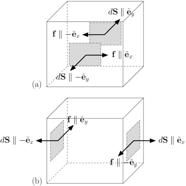
Figure 2: Soft shears in biaxial elastomers. The force $\bm{{\rm f}}$ exerted across an infinitesimal surface element $d\bm{{\rm S}}$ is $f_{i}=\sigma_{ij}dS_{j}$. There are no restoring forces for (a) external forces along $\pm\tilde{\bm{{\rm e}}}_{x}$ applied to opposing surfaces with normal along $\pm\tilde{\bm{{\rm e}}}_{y}$, and (b) for external forces along $\pm\tilde{\bm{{\rm e}}}_{y}$ applied to surfaces with normal along $\pm\tilde{\bm{{\rm e}}}_{x}$.

Note that there is an interesting parallel between the biaxial smectics considered here and biaxial nematics formed spontaneously from an isotropic elastomer. Warner and Kutter warner_kutter_2002 predicted that these biaxial nematics have many soft modes, and one of these is identical to the soft mode of biaxial smectics discussed above. Finally, we observe that a biaxial smectic has the same point-group symmetry $D_{2h}$ as an orthorhombic crystal. However, because it is formed via spontaneous symmetry breaking from a state with $D_{\infty h}$, unlike an equilibrium orthorhombic crystal, it exhibits soft elasticity in the $xy$-plane. An orthorhombic state can be reached via a symmetry-breaking transition from a tetragonal state, which exhibits square symmetry in the $xy$ plane. Rather than exhibiting the soft elasticity discussed above such an orthorhombic system exhibits martinsitic elasticity martensite in which domains of different orientation are produced in response to stress perpendicular to the stretch direction in the $xy$ plane.

III.3 Rotational invariance and soft extensional strains

In addition to the softness under $u_{xy}^{\prime}$ shears, the new phase is, provided that the experimental boundary condition are right, soft with respect to certain extensional strains. In the following paragraphs, we will discuss this softness in some detail. The mechanism at work here is intimately related to a mechanism leading to a similar softness in nematic elastomers, and thus our reasoning will follow closely well known arguments for nematic elastomers golubovic_lubensky_89 ; LubenskyXin2002 . The form of these soft strains depends only on symmetry and the nature of the broken-symmetry phase; it is not restricted to small strains or to systems described by a Landau expansion of the free energy. First, we will consider global rotations in the $xy$-plane of the reference space of our biaxial elastomers. On the one hand this will prepare the ground for understanding the softness of extensional strains, and on the other hand, it will allow us to understand the vanishing of the elastic constant $C_{xyxy}$ from a somewhat different perspective. Then we calculate the energy cost of soft extensional strains and finally we comment on experimental implications.

We saw in Sec. III.1 that the direction of the spontaneous anisotropy $xy$-plane, or in other words, the direction of the $c$-director $\tilde{\bm{{\rm c}}}$, is arbitrary. Thus, equilibrium states characterized, respectively, by $\underline{\underline{u}}^{0}$ and $\underline{\underline{O}}_{R,z}\underline{\underline{u}}^{0}\,\underline{\underline{O}}_{R,z}^{-1}$, where $\underline{\underline{O}}_{R,z}$ describes an arbitrary rotation in the reference space about the $z$ axis, must have the same energy. With

$$\underline{\underline{O}}_{R,z}=\left(\begin{array}[]{ccc}\cos\vartheta&-\sin\vartheta&0\\ \sin\vartheta&\cos\vartheta&0\\ 0&0&1\end{array}\right)$$ (50)

describing a counterclockwise rotation of vectors in the reference space through $\vartheta$ about the $z$-axis, the strain

$$\underline{\underline{u}}^{\prime}(\vartheta) =\big{(}\underline{\underline{\Lambda}}^{0T}\big{)}^{-1}\big{[}\underline{\underline{O}}_{R,z}\,\underline{\underline{u}}^{0}\,\underline{\underline{O}}_{R,z}^{-1}-\underline{\underline{u}}^{0}\big{]}\big{(}\underline{\underline{\Lambda}}^{0}\big{)}^{-1}$$ (51a)

$$=\frac{r_{\perp}-1}{4}\left(\begin{array}[]{ccc}-r_{\perp}^{-1}(1-\cos 2\vartheta)&r_{\perp}^{-1/2}\sin 2\vartheta&0\\ r_{\perp}^{-1/2}\sin 2\vartheta&1-\cos 2\vartheta&0\\ 0&0&0\end{array}\right)$$ (51e)

must not cost any elastic energy. Our elastic energy density (III.2) contains only second-order terms in $u_{ij}^{\prime}$, and hence it can at best be invariant with respect to infinitesimal rotations footnoteSmallRotation . However, even for infinitesimal $\vartheta$, the strain $\underline{\underline{u}}^{\prime}(\vartheta)$ has nonzero components, namely

$$u^{\prime}_{xy}(\vartheta)=u^{\prime}_{yx}(\vartheta)=\frac{r_{\perp}-1}{2\sqrt{r_{\perp}}}\,\vartheta\,.$$ (52)

Thus, as it does in Eq. (III.2), the elastic constant $C_{xyxy}$ of the term (45) must indeed vanish, and this vanishing can be understood as a result of the spontaneous symmetry breaking in the $xy$-plane.

The existence of zero-energy strains that reproduce rotations in the reference space has consequences reaching further then just the softness with respect to shear strains $u^{\prime}_{xy}$, viz. depending on the experimental boundary conditions, extensional strains $u^{\prime}_{xx}$ and $u^{\prime}_{yy}$ can also be soft. If the boundary conditions are such that no relaxation of strains is allowed, then strains $u^{\prime}_{xx}$ and $u^{\prime}_{yy}$ will cost an elastic energy proportional to $(u^{\prime}_{xx})^{2}$ and $(u^{\prime}_{yy})^{2}$, respectively. If, however, strain relaxation is allowed and one imposes for example $u^{\prime}_{yy}$ with the right sign, then $u^{\prime}_{xx}$ and $u^{\prime}_{xy}$ can relax under the right circumstances to produce the zero-energy strain of Eq. (51), i.e., to make $u^{\prime}_{yy}$ a soft deformation.

To discuss this in more detail, let us assume for concreteness that the anisotropy in the $xy$-plane is positive, $r_{\perp}>1$. Then it follows from Eq. (51) that $u^{\prime}_{yy}$ is positive and that $u^{\prime}_{xx}$ is negative for soft strains and that we consequently can only have soft elasticity for $u^{\prime}_{yy}>0$ and $u^{\prime}_{xx}<0$. Let us consider here as an example a strain with $u^{\prime}_{yy}>0$, i.e., a stretch of the sample along $y$. Comparison with Eq. (51) shows that, if strain relaxation is allowed and $u^{\prime}_{xx}$ and $u^{\prime}_{xy}$ relax to

$$u^{\prime}_{xx} =-r_{\perp}^{-1}u^{\prime}_{yy}\,,$$ (53a)

$$u^{\prime}_{xy} =\pm\sqrt{\frac{u^{\prime}_{yy}(r_{\perp}-1-2u^{\prime}_{yy})}{2r_{\perp}}}\,,$$ (53b)

then $u^{\prime}_{yy}$ is converted into a zero-energy rotation through an angle

$$\vartheta=\pm\frac{1}{2}\sin^{-1}\left[\frac{2}{r_{\perp}-1}\sqrt{2u^{\prime}_{yy}(r_{\perp}-1-2u^{\prime}_{yy})}\right].$$ (54)

Thus, $u^{\prime}_{yy}$ costs no elastic energy as long as $0<u^{\prime}_{yy}<(r_{\perp}-1)/2$.

When $u^{\prime}_{yy}$ is increased from zero, $\vartheta$ increases from zero until it reaches $\pi/2$ at $u^{\prime}_{yy}=(r_{\perp}-1)/2$ [and $u^{\prime}_{xx}=(r_{\perp}^{-1}-1)/2$, $u^{\prime}_{xy}=0$] at which point, the deformation tensor defined by $\Lambda^{\prime}_{0ij}=\partial R_{i}/\partial x^{\prime}_{j}$ is

$$\underline{\underline{\Lambda}}^{\prime}_{0}=\left(\begin{array}[]{ccc}r_{\perp}^{-1/2}&0&0\\ 0&r_{\perp}^{1/2}&0\\ 0&0&1\end{array}\right),$$ (55)

which leads via $\Lambda_{ij}=\Lambda_{ik}^{0}\Lambda^{\prime}_{0kj}$ to an overall deformation

$$\underline{\underline{\Lambda}}=\left(\begin{array}[]{ccc}\Lambda_{yy}^{0}&0&0\\ 0&\Lambda_{yy}^{0}\sqrt{r_{\perp}}&0\\ 0&0&\Lambda_{zz}^{0}\end{array}\right)$$ (56)

relative the original uniaxial state. Thus, at $\vartheta=\pi/2$, $\Lambda_{ij}$ is identical to $\Lambda_{ij}^{0}$ except with $\Lambda_{xx}^{0}=\sqrt{r_{\perp}}\Lambda_{yy}^{0}$ replaced by $\Lambda^{0}_{yy}$ and $\Lambda_{yy}^{0}$ replaced by $\Lambda_{xx}^{0}$, i.e., the $x$ and $y$ axes have been interchanged in going from $\vartheta=0$ to $\vartheta=\pi/2$. In the process, $\tilde{\bm{{\rm c}}}$ rotates from being parallel the $x$-axis to being parallel to the $y$-axis c_rot .

For $u_{yy}^{\prime}>(r_{\perp}-1)/2$, there is no real solution for $\vartheta$, and a further increase in $u_{yy}^{\prime}$, measured by $\delta u_{yy}^{\prime}=u_{yy}^{\prime}-(r_{\perp}-1)/2$, which stretches the system along the space-fixed $y$-axis, cost energy. Since the anisotropy axis is now along the $y$- rather than the $x$-axis, this stretching costs the same energy as it would have cost to stretch the original system with anisotropy axis along the space-fixed $x$-axis by the same amount. The $yy$-component of the strain relative to the state with $\vartheta=\pi/2$ is $\Delta u_{yy}^{\prime}=(\Lambda_{0yy}^{\prime})^{-2}\delta u_{yy}^{\prime}=r_{\perp}^{-1}\delta u_{yy}^{\prime}$. Thus, because the $x$- and $y$-axes have been interchanged, the free energy as a function of $u_{yy}^{\prime}$ is

$$f_{D_{2h}}^{\text{soft}} =\left\{\begin{array}[]{lcc}0&\mbox{for}&\delta u^{\prime}_{yy}<0\,,\\ \textstyle{\frac{1}{2}}\,Y_{x}\,(\delta u^{\prime}_{yy})^{2}&\mbox{for}&\delta u^{\prime}_{yy}>0\,.\end{array}\right.$$ (59)

where

$$Y_{x} =\frac{1}{r_{\perp}^{2}}\,\bigg{\{}C_{xxxx}$$

$$-\frac{C_{yyyy}C_{zzxx}^{2}+C_{zzzz}C_{xxyy}^{2}-2C_{xxyy}C_{xxzz}C_{yyzz}}{C_{yyyy}C_{zzzz}-C_{yyzz}^{2}}\bigg{\}}.$$ (60)

is the is Young’s modulus for stretching along the anisotropy axis in the $xy$-plane (originally along $x$).

Equation (59) has tangible implications for the stress-strain behavior of soft biaxial elastomers. The stress that is usually measured in experiments is the engineering stress, i. e., the force per unit area of the reference state. For the extensional strain under discussion here, the engineering stress stress_tensors is to leading order

$$\sigma^{\text{eng}}_{yy} =\frac{\partial f_{D_{2h}}^{\text{soft}}}{\partial\Lambda^{\prime}_{yy}}=\left\{\begin{array}[]{lcc}0&\mbox{for}&\Lambda^{\prime}_{yy}<\sqrt{r_{\perp}}\\ Y_{x}\,\Lambda^{\prime}_{0yy}\,\delta u_{yy}^{\prime}&\mbox{for}&\Lambda^{\prime}_{yy}>\sqrt{r_{\perp}}\end{array}\right..$$ (63)

For $\Lambda_{yy}^{\prime}$ near $\Lambda_{0yy}^{\prime}$, $\delta u_{yy}^{\prime}\approx\Lambda_{0yy}^{\prime}(\Lambda_{yy}^{\prime}-\Lambda_{0yy}^{\prime})$, and $\sigma^{\text{eng}}_{yy}\approx Y_{x}(\Lambda_{yy}^{\prime}-\Lambda_{0yy}^{\prime})$. Figure 3 depicts the dependence of $\sigma^{\text{eng}}_{yy}$ on $\Lambda^{\prime}_{yy}$. From $\Lambda^{\prime}_{yy}=0$ up to a critical deformation $\Lambda^{\prime}_{0yy}=\sqrt{r_{\perp}}$ the stress is zero. Above the critical deformation, $\sigma^{\text{eng}}_{yy}$ grows linearly from zero.

Figure 3: Schematic plot (arbitrary units) of the engineering stress $\sigma^{\text{eng}}_{yy}$ versus the deformation $\Lambda^{\prime}_{yy}$ for a soft biaxial elastomer with an equilibrium order in the $xy$-plane along $x$ and positive anisotropy, $r_{\perp}>0$. Up to a critical deformation $\Lambda^{\prime}_{0yy}=\sqrt{r_{\perp}}$ the sample responds to the deformation merely by rotating $\tilde{\bm{{\rm c}}}$ and consequently the stress is zero. Above $\Lambda^{\prime}_{0yy}$ the sample stretches along the new direction $y$ of the c-director and $\sigma^{\text{eng}}_{yy}$ grows linearly for small $\Lambda_{yy}^{\prime}-\Lambda_{0yy}^{\prime}$.

IV Smectic-$C$ elastomers – strain-only theory

In this section we use the strain-only theory to study the phase transition from a uniaxial Sm$A$ elastomer to a Sm$C$ elastomer when $C_{5}$ becomes negative in response to a Sm$C$-ordering of the mesogenic component.

IV.1 Phase transition from uniaxial to smectic-$C$ elastomers

When $C_{5}$ is driven negative, the uniaxial state becomes unstable to shear in the planes containing the anisotropy axis, and the uniaxial energy (II) must be augmented with higher-order terms involving $u_{az}$ to stabilize the system:

$$f_{\text{uni}}^{(2)} =f_{\text{uni}}+D_{1}\,u_{zz}u_{az}^{2}+D_{2}\,u_{ii}u_{az}^{2}+D_{3}\,\hat{u}_{ab}u_{az}u_{bz}$$

$$+E\,(u_{az}^{2})^{2},$$ (64)

where we omit all unimportant symmetry-compatible higher-order terms and we use $u_{zz}$ and $u_{ii}$ rather than $\eta_{z}$ and $\eta$. To study the ordered phase of this free energy when $C_{5}<0$, we proceed in much the same way as we did for the biaxial state of $f_{\text{uni}}^{(1)}$. Using Eq. (II) for $f_{\text{uni}}$, we complete squares to write $f_{\text{uni}}^{(2)}$ as the sum

$$f_{\text{uni}}^{(2)}=f_{\text{uni}}^{(2,1)}+f_{\text{uni}}^{(2,2)},$$ (65)

of the two terms

$$f_{\text{uni}}^{(2,1)} =\textstyle{\frac{1}{2}}\,C_{1}\,w_{zz}^{2}+C_{2}\,w_{ii}w_{zz}+\textstyle{\frac{1}{2}}\,C_{3}\,w_{ii}^{2}+C_{4}\,w_{ab}^{2}\,,$$ (66a)

$$f_{\text{uni}}^{(2,2)} =C_{5}\,u_{az}^{2}+E_{R}\,(u_{az}^{2})^{2}\,,$$ (66b)

where $E_{R}$, which we assume to be positive, is a renormalized version of $E$,

$$E_{R}=E-\textstyle{\frac{1}{2}}\sigma^{2}\,C_{1}-\sigma\tau\,C_{2}-\textstyle{\frac{1}{2}}\tau^{2}\,C_{3}-\textstyle{\frac{1}{2}}\omega^{2}\,C_{4}\,,$$ (67)

and where

$$w_{zz}=u_{zz}-\sigma u_{az}^{2}\,,$$ (68a)

$$w_{ii}=u_{ii}-\tau u_{az}^{2}\,,$$ (68b)

$$w_{ab}=\hat{u}_{ab}-\omega\left(u_{az}u_{bz}-\textstyle{\frac{1}{2}}\delta_{ab}u_{cz}^{2}\right)\,.$$ (68c)

The coefficients in Eqs. (67) and (68) are given by

$$\left(\begin{array}[]{c}\sigma\\ \tau\end{array}\right)=\frac{-1}{C_{1}\,C_{3}-C_{2}^{2}}\left(\begin{array}[]{c}C_{3}D_{1}-C_{2}D_{2}\\ C_{1}D_{2}-C_{2}D_{1}\end{array}\right)$$ (73)

and

$$\omega=-\frac{D_{3}}{2\,C_{4}}\,.$$ (74)

In the limit $C_{3}\to\infty$ the coefficient $\tau$ vanishes whereas $\sigma$, $\omega$, and $E_{R}$ remain finite.

The equilibrium value $u_{az}^{0}$ of $u_{az}$ is determined by minimizing $f_{\text{uni}}^{(2,2)}$, which has $xy$ symmetry. Provided that we choose our coordinate system so that its $x$-axis is along the direction of ordering, the corresponding equation of state,

$$C_{5}\,u_{az}^{0}+2\,E_{R}\,u_{az}^{0}(u_{bz}^{0})^{2}=0,$$ (75)

leads to

$$u_{yz}^{0}=0\quad\mbox{for}\quad C_{5}>0\quad\mbox{and}\quad C_{5}<0$$ (76)

and

$$S\equiv u_{xz}^{0}=\left\{\begin{array}[]{ccc}0&\quad\mbox{for}&C_{5}>0\,,\\ \pm\sqrt{-C_{5}/(2E_{R})}&\quad\mbox{for}&C_{5}<0\,.\end{array}\right.$$ (79)

From Eqs. (66a) and (68) the other components of $\underline{\underline{u}}^{0}$ follow as

$$u_{xx}^{0}=\textstyle{\frac{1}{2}}\,(\tau+\omega-\sigma)\,S^{2}\,,$$ (80a)

$$u_{yy}^{0}=\textstyle{\frac{1}{2}}\,(\tau-\omega-\sigma)\,S^{2}\,,$$ (80b)

$$u_{zz}^{0}=\sigma\,S^{2}\,.$$ (80c)

We learn that, unlike the biaxial case, $\underline{\underline{u}}^{0}$ is not diagonal; it has nonvanishing $xz$ and $zx$ components, which implies $C_{2h}$ rather than $D_{2h}$ symmetry.

As already pointed out in Sec. III, an equilibrium strain tensor determines the corresponding equilibrium deformation tensor only up to global rotations in the target space. Here we choose our coordinate system in the target space so that the transition from the $D_{2\infty}$ to the $C_{2h}$ state corresponds to a simple shear as shown in Fig. 1, i.e., we choose the target space coordinates so that $\tan\phi=\Lambda_{xz}^{0}/\Lambda_{zz}^{0}$ is nonzero but $\Lambda_{zx}^{0}=0$. Then the only nonzero components of $\underline{\underline{\Lambda}}^{0}$ are

$$\Lambda_{xx}^{0} =\sqrt{1+2u_{xx}^{0}}=\sqrt{1+(\tau+\omega-\sigma)\,S^{2}}\,,$$ (81a)

$$\Lambda_{yy}^{0} =\sqrt{1+2u_{yy}^{0}}=\sqrt{1+(\tau-\omega-\sigma)\,S^{2}}\,,$$ (81b)

$$\Lambda_{xz}^{0} =2\,\frac{u_{xz}^{0}}{\Lambda_{xx}^{0}}=\frac{2\,S}{\sqrt{1+(\tau+\omega-\sigma)\,S^{2}}}\,,$$ (81c)

$$\Lambda_{zz}^{0} =\sqrt{1+2u_{zz}^{0}-(\Lambda_{xz}^{0})^{2}}$$

$$=\sqrt{1+2\,\frac{(\sigma-2)\,S^{2}+(\tau+\omega-\sigma)\,\sigma\,S^{4}}{1+(\tau+\omega-\sigma)\,S^{2}}}\,.$$ (81d)

IV.2 Elasticity of the smectic-$C$ phase

Next we expand the elastic free energy density about the equilibrium state. The expansion of $f_{\text{uni}}^{(2,1)}$ [Eq. (66a)] is particularly simple and leads to

$$\delta f_{\text{uni}}^{(2,1)} =\textstyle{\frac{1}{2}}\,C_{1}\,(\delta w_{zz})^{2}+C_{2}\,\delta w_{ii}\delta w_{zz}+\textstyle{\frac{1}{2}}\,C_{3}\,(\delta w_{ii})^{2}$$

$$+C_{4}\,(\delta w_{ab})^{2}$$ (82)

with

$$\delta w_{zz}=\delta u_{zz}-2\sigma S\,\delta u_{xz}\,,$$ (83a)

$$\delta w_{ii}=\delta u_{ii}-2\tau S\,\delta u_{xz}\,,$$ (83b)

$$\delta w_{xx}=-\delta w_{yy}=\textstyle{\frac{1}{2}}\,(\delta u_{xx}-\delta u_{yy})-\omega S\,\delta u_{xz}\,,$$ (83c)

$$\delta w_{xy}=\delta w_{yx}=\delta u_{xy}-\omega S\,\delta u_{yz}\,.$$ (83d)

Expanding $f_{\text{uni}}^{(2,2)}$ [Eq. (66b)], we find that

$$\delta f_{\text{uni}}^{(2,2)}=4E_{R}S^{2}(\delta u_{xz})^{2}$$ (84)

is independent of $\delta u_{yz}$, and we might naively expect the system to exhibit softness with respect to $u_{yz}$. This, however, is not the case because $f_{\text{uni}}^{(2,1)}$ depends on $\delta u_{yz}$ via the relative strain (83d). Thus, the softness of the ordered phase with $C_{2h}$ symmetry is more subtle than that of the biaxial phase with $D_{2h}$ symmetry, as we will discuss in more detail further below. Assembling the contributions (IV.2) and (84) we obtain for the entire elastic free energy density to harmonic order

$$\delta f^{(2)} =2C_{4}[\delta u_{xy}-\omega S\,\delta u_{yz}]^{2}+\textstyle{\frac{1}{2}}\,[C_{1}+2C_{2}+C_{3}]\,(\delta u_{zz})^{2}+4ES^{2}\,(\delta u_{xz})^{2}+\textstyle{\frac{1}{2}}\,[C_{3}+C_{4}]\,\{(\delta u_{xx})^{2}+(\delta u_{yy})^{2}\}$$

$$+[C_{2}+C_{3}]\delta u_{zz}\{\delta u_{xx}+\delta u_{yy}\}+[C_{3}-C_{4}]\delta u_{xx}\delta u_{yy}+(2D_{2}+D_{3})S\,\delta u_{xx}\delta u_{xz}+(2D_{2}-D_{3})S\,\delta u_{yy}\delta u_{xz}$$

$$+2(D_{1}+D_{2})S\,\delta u_{zz}\delta u_{xz}\,.$$ (85)

Our remaining step in deriving the elastic free energy density of Sm$C$ elastomers is to change from the variables of the old uniaxial state to those of the new state by switching from $\delta\underline{\underline{u}}$ to the new strain tensor $\underline{\underline{u}}^{\prime}$ as defined in Eq. (43). With the equilibrium deformation tensor as stated in Eqs. (81) we obtain after some algebra

$$f_{C_{2h}}^{\text{soft}}=\textstyle{\frac{1}{2}}\,\bar{C}\left[\cos\theta\,u^{\prime}_{xy}+\sin\theta\,u^{\prime}_{yz}\right]^{2}+\textstyle{\frac{1}{2}}\,C_{zzzz}\,(u^{\prime}_{zz})^{2}$$

$$+\textstyle{\frac{1}{2}}\,C_{xzxz}\,(u^{\prime}_{xz})^{2}+C_{zzxx}\,u^{\prime}_{zz}u^{\prime}_{xx}+C_{zzyy}\,u^{\prime}_{zz}u^{\prime}_{yy}$$

$$+\textstyle{\frac{1}{2}}\,C_{xxxx}\,(u^{\prime}_{xx})^{2}+\textstyle{\frac{1}{2}}\,C_{yyyy}\,(u^{\prime}_{yy})^{2}+C_{xxyy}\,u^{\prime}_{xx}u^{\prime}_{yy}$$

$$+C_{xxxz}\,u^{\prime}_{xx}u^{\prime}_{xz}+C_{yyxz}\,u^{\prime}_{yy}u^{\prime}_{xz}+C_{zzxz}\,u^{\prime}_{zz}u^{\prime}_{xz}\,,$$ (86)

where the angle $\theta$ and the elastic constants depend on the original elastic constants in Eq. (IV.1) and $S$ so that one retrieves the uniaxial energy density (II) for $S\to 0$. The explicit results for these quantities, which are somewhat lengthy, can be found in Appendix B. In the incompressible limit, the specifics of $\theta$ and the elastic constants get modified, however, without changing the form of Eq. (IV.2).

Having established the result (IV.2), we are now in the position to discuss the anticipated softness of the new state. Our first observation is that the elastic energy density of Eq. (IV.2) has only 12 (including $\theta$) rather than the 13 independent elastic constants of conventional monolinic solids triclinic . That is because here there are only two rather than three independent elastic constants in the subspace spanned by $u^{\prime}_{xy}$ and $u^{\prime}_{yz}$. Below, we present two derivations of this result.

In the first derivation, we exploit the fact that $\cos\theta u^{\prime}_{xy}+\sin\theta u^{\prime}_{yz}$ can be viewed as the dot product of the “vectors” $\vec{v}=(u^{\prime}_{xy},u^{\prime}_{yz})$ and $\vec{e}_{1}=(\cos\theta,\sin\theta)$. Thus, the first term in Eq. (IV.2),

$$\textstyle{\frac{1}{2}}\,\bar{C}\left[\cos\theta\,u^{\prime}_{xy}+\sin\theta\,u^{\prime}_{yz}\right]^{2}=\textstyle{\frac{1}{2}}\,\bar{C}\,(\vec{e}_{1}\cdot\vec{v})^{2}\,,$$ (87)

is independent of $\vec{e}_{2}\cdot\vec{v}$, where

$$\vec{e}_{2}=(-\sin\theta,\cos\theta)$$ (88)

is the vector perpendicular to $\vec{e}_{1}$. Thus, distortions of the form $-\sin\theta u^{\prime}_{xy}+\cos\theta u_{yz}=\vec{e}_{2}\cdot\vec{v}$, i.e, distortions with $\vec{v}$ along $\vec{e}_{2}$, cost no elastic energy. A manifestation of this softness is that certain stresses cause no restring force and thus lead to large deformations. To find these stresses we take the derivative of the elastic energy density (IV.2) with respect to $u^{\prime}_{xy}$ and $u^{\prime}_{yz}$ which tells us that

$$-\sin\theta\,\sigma_{xy}+\cos\theta\,\sigma_{zy}=\vec{e}_{2}\cdot\vec{w}=0\,,$$ (89)

where again, $\sigma_{ij}$ is the second Piola-Kirchhoff stress tensor and where we have introduced the “vector”

$$\vec{w}=(\sigma_{xy},\sigma_{zy})$$ (90)

in the $xz$-plane. Equation (89) means that there are no restoring forces for external forces in the $xz$-plane along $\pm\tilde{\bm{{\rm e}}}_{2}\equiv\pm(-\sin\theta,0,\cos\theta)$ applied to opposing surfaces with normal along $\pm\tilde{\bm{{\rm e}}}_{y}$, and there no restoring forces for external forces along $\pm\tilde{\bm{{\rm e}}}_{y}$ applied to surfaces with normal along $\pm\tilde{\bm{{\rm e}}}_{2}$. These kinds of stresses are depicted in Fig. 4.

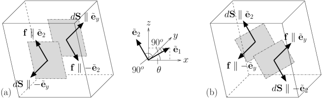
Figure 4: Soft distortions of Sm$C$ elastomers. There are no restoring forces (a) for external forces in the $xz$-plane along $\pm\tilde{\bm{{\rm e}}}_{2}$ applied to opposing surfaces with normal along $\pm\tilde{\bm{{\rm e}}}_{y}$, and (b) for external forces along $\pm\tilde{\bm{{\rm e}}}_{y}$ applied to surfaces with normal along $\pm\tilde{\bm{{\rm e}}}_{2}$.

A second derivation of the softness of the Sm$C$ phase involves a transformation to a rotated coordinate system, as described in Eq. (5), in which the first term in Eq. (IV.2) is diagonal. The components $x^{\prime\prime}_{i^{\prime}}$ of a reference-space vector $\bm{{\rm x}}^{\prime}$ expressed with respect to a rotated basis $\{\tilde{\bm{{\rm e}}}_{i^{\prime}}^{\prime}|i^{\prime}=x^{\prime},y^{\prime},z^{\prime}\}$, where $\tilde{\bm{{\rm e}}}_{i^{\prime}}^{\prime}=O_{R,y;i^{\prime}j}\tilde{\bm{{\rm e}}}_{j}$ with

$$\underline{\underline{O}}_{R,y}=\left(\begin{array}[]{ccc}\cos\theta&0&\sin\theta\\ 0&1&0\\ -\sin\theta&0&\cos\theta\end{array}\right)$$ (94)

describing a counterclockwise rotation of the reference-space basis about the $y$-axis, are simply $x^{\prime\prime}_{i}=O_{R,y;ij}\,x^{\prime}_{j}$. The components of the strain matrix expressed in the rotated basis are $u^{\prime\prime}_{i^{\prime}j^{\prime}}=\tilde{\bm{{\rm e}}}_{i^{\prime}}^{\prime}\cdot\underline{\underline{u}}^{\prime}\cdot\tilde{\bm{{\rm e}}}_{j^{\prime}}^{\prime}=O_{R,y;i^{\prime}i}u_{ij}O_{R,y;jj^{\prime}}^{T}$, from which we obtain via Eq. (10) that $u^{\prime\prime}_{x^{\prime},y^{\prime}}=\cos\theta\,u^{\prime}_{xy}+\sin\theta\,u^{\prime}_{yz}$ and $u^{\prime\prime}_{y^{\prime},z^{\prime}}=-\sin\theta\,u^{\prime}_{xy}+\cos\theta\,u^{\prime}_{yz}$. Thus, taking $\theta$ to be the angle appearing in Eq. (IV.2) and dropping the double-prime from the strains, we obtain

$$f_{C_{2h}}^{\text{soft}}=\textstyle{\frac{1}{2}}\,C_{x^{\prime}y^{\prime}x^{\prime}y^{\prime}}\,(u_{x^{\prime}y^{\prime}})^{2}+\textstyle{\frac{1}{2}}\,C_{z^{\prime}z^{\prime}z^{\prime}z^{\prime}}\,(u_{z^{\prime}z^{\prime}})^{2}$$

$$+\textstyle{\frac{1}{2}}\,C_{x^{\prime}z^{\prime}x^{\prime}z^{\prime}}\,(u_{x^{\prime}z^{\prime}})^{2}+C_{z^{\prime}z^{\prime}x^{\prime}x^{\prime}}\,u_{z^{\prime}z^{\prime}}u_{x^{\prime}x^{\prime}}$$

$$+C_{z^{\prime}z^{\prime}y^{\prime}y^{\prime}}\,u_{z^{\prime}z^{\prime}}u_{y^{\prime}y^{\prime}}+\textstyle{\frac{1}{2}}\,C_{x^{\prime}x^{\prime}x^{\prime}x^{\prime}}\,(u_{x^{\prime}x^{\prime}})^{2}$$

$$+\textstyle{\frac{1}{2}}\,C_{y^{\prime}y^{\prime}y^{\prime}y^{\prime}}\,(u_{y^{\prime}y^{\prime}})^{2}+C_{x^{\prime}x^{\prime}y^{\prime}y^{\prime}}\,u_{x^{\prime}x^{\prime}}u_{y^{\prime}y^{\prime}}$$

$$+C_{x^{\prime}x^{\prime}x^{\prime}z^{\prime}}\,u_{x^{\prime}x^{\prime}}u_{x^{\prime}z^{\prime}}+C_{y^{\prime}y^{\prime}x^{\prime}z^{\prime}}\,u_{y^{\prime}y^{\prime}}u_{x^{\prime}z^{\prime}}$$

$$+C_{z^{\prime}z^{\prime}x^{\prime}z^{\prime}}\,u_{z^{\prime}z^{\prime}}u_{x^{\prime}z^{\prime}}\,.$$ (95)

for the elastic energy density of Sm$C$ elastomers in the rotated coordinates. Note that, in this coordinate system, the elastic constants $C_{x^{\prime}y^{\prime}y^{\prime}z^{\prime}}$ and $C_{y^{\prime}z^{\prime}y^{\prime}z^{\prime}}$ are zero, and the elastic energy does not depend at all on $u_{y^{\prime}z^{\prime}}$. $C_{x^{\prime}y^{\prime}x^{\prime}y^{\prime}}$ is identical to $\bar{C}$ and $C_{y^{\prime}y^{\prime}y^{\prime}y^{\prime}}=C_{yyyy}$. The remaining new elastic constants are non-vanishing conglomerates of the elastic constants defined via Eq. (IV.2) and sines and cosines of $\theta$. We refrain here from stating further specifics to save some space and because calculating these specifics is a straightforward exercise.

The vanishing of $C_{x^{\prime}y^{\prime}y^{\prime}z^{\prime}}$ and $C_{y^{\prime}z^{\prime}y^{\prime}z^{\prime}}$ means that Sm$C$ elastomers are soft with respect to shears in the $y^{\prime}z^{\prime}$-plane. If one can cut a rectangular sample with faces perpendicular to the $\tilde{\bm{{\rm e}}}_{i^{\prime}}^{\prime}$, then there are no restoring forces for external forces along $\pm\tilde{\bm{{\rm e}}}_{z^{\prime}}^{\prime}$ applied to opposing surfaces with normal along $\pm\tilde{\bm{{\rm e}}}_{y^{\prime}}^{\prime}$, and for external forces along $\pm\tilde{\bm{{\rm e}}}_{y^{\prime}}^{\prime}$ applied to surfaces with normal along $\pm\tilde{\bm{{\rm e}}}_{z^{\prime}}^{\prime}$. This softness can be visualized as in Fig. 2 with $\tilde{\bm{{\rm e}}}_{x}$ replaced by $\tilde{\bm{{\rm e}}}_{z^{\prime}}^{\prime}$ and $\tilde{\bm{{\rm e}}}_{y}$ replaced by $\tilde{\bm{{\rm e}}}_{y^{\prime}}^{\prime}=\tilde{\bm{{\rm e}}}_{y}$.

Before we go on, let us finally comment on the impact of the softness on the phonon spectrum of Sm$C$ elastomers. A comprehensive discussion of the phonon spectrum of course requires a dynamical theory of smectic elastomers. This is beyond the scope of this paper and makes the topic of a separate publication stenull_lubensky_SmCdynamics . Our current theory allows us to address static phonons. To this end we switch to Fourier space fourierTransformation and re-express the elastic energy density (IV.2) in terms of the Fourier transform $\widetilde{\bm{{\rm u}}}(\bm{{\rm q}})$ with respect to $\bm{{\rm x}}^{\prime}$ of the displacement field $\bm{{\rm u}}^{\prime}(\bm{{\rm x}}^{\prime})=\bm{{\rm R}}^{\prime}(\bm{{\rm x}}^{\prime})-\bm{{\rm x}}^{\prime}$. Neglecting the non-linear part of the strains, cf. Eq. (9), this yields a Fourier transformed elastic energy density $\widetilde{f}_{C_{2h}}^{\text{soft}}$ harmonic in $\widetilde{\bm{{\rm u}}}$ and the wavevector. With $\widetilde{u}_{x}=\widetilde{u}_{z}=q_{y}=0$, $\widetilde{f}_{C_{2h}}^{\text{soft}}$ reduces to

$$\widetilde{f}_{C_{2h}}^{\text{soft}}=\textstyle{\frac{1}{8}}\,\bar{C}\,(\cos\theta\,q_{x}+\sin\theta\,q_{z})^{2}\,\widetilde{u}_{y}^{2}\,.$$ (96)

Hence, the energy cost is zero for phonon displacements $\widetilde{\bm{{\rm u}}}=(0,\widetilde{u}_{y},0)$ parallel to $\tilde{\bm{{\rm e}}}_{y}$ with wavevector $\bm{{\rm q}}\parallel\tilde{\bm{{\rm e}}}_{z^{\prime}}$. By similar means one also finds that there is no energy cost for $\widetilde{\bm{{\rm u}}}\parallel\tilde{\bm{{\rm e}}}_{z^{\prime}}$ with $\bm{{\rm q}}\parallel\tilde{\bm{{\rm e}}}_{y}$. This softness of these phonons has tangible implications on the dynamics in that it leads, e.g., to a vanishing of the corresponding sound velocities stenull_lubensky_SmCdynamics .

An interesting question that we have left aside so far is, of course, whether Sm$C$ elastomers are, like nematics or biaxial smectics, soft with respect to certain extensional strains. We will postpone this question to Sec. V until after we have developed our strain-and-director model for Sm$C$ elastomers. This will then allow us to discuss soft deformations and strains more comprehensively including their impact on the director.

V Smectic-$C$ elastomers – theory with strain and director

Our second theory for Sm$C$ elastomers, to be presented in this section, explicitly accounts for the smectic layers and for the director $\bm{{\rm n}}$. It generalizes the achiral limit of the continuum theory by Terentjev and Warner terentjev_warner_SmC_1994 in a formalism that ensures invariance with respect to arbitrary rather than infinitesimal rotations of both the director and mass points. We will see as we move along that the properties of the transition to the Sm$C$ phase predicted by this theory are identical to those of the strain-only theory, discussed in the preceding section, in which $C_{5}$ goes to zero.

V.1 Reference- and target-space variables and the polar decomposition theorem

In traditional uncrosslinked liquid crystals, there is no reference space, and all physical fields like the smectic layer-displacement field $U$, the layer normal $\bm{{\rm N}}$, and the Frank director $\bm{{\rm n}}$ are defined at real, i.e., target-space points $\bm{{\rm R}}$, and they transform as scalars, vectors, and tensors under rotations in the target space. In the Lagrangian theory of elasticity, fields are defined at reference space points $\bm{{\rm x}}$, and they transform into themselves under the symmetry operations of that space. To develop a comprehensive theory of liquid-crystalline elastomers, it is necessary to combine target-space liquid crystalline fields and reference-space elastic variables to produce scalars that are invariant under arbitrary rotations in the target space and under symmetry operations of the reference space. This requires that we be able to represent vectors and tensors in either space LubenskyXin2002 .

To be more specific, let $\bm{{\rm b}}$ be a target-space vector, which by definition transforms under rotations to $\bm{{\rm b}}^{\prime}=\underline{\underline{O}}_{T}\bm{{\rm b}}$, and let $\tilde{\bm{{\rm b}}}$ be a reference-space vector, which transforms to $\tilde{\bm{{\rm b}}}^{\prime}=\underline{\underline{O}}_{R}\tilde{\bm{{\rm b}}}$. Recall that both reference- and target-space vectors exist in the same physical Euclidean space $\cal E$. Therefore, there must be a transformation that converts a given reference-space vector to a target-space vector and vice versa while preserving length. This transformation is provided by the deformation matrix $\underline{\underline{\Lambda}}$ and the matrix polar decomposition theorem HornJoh1991 , which states that any non-singular square matrix can be expressed as the product of a rotation matrix and a symmetric matrix. If $\tilde{\bm{{\rm b}}}$ is a reference-space vector, then $\underline{\underline{\Lambda}}\tilde{\bm{{\rm b}}}$ is a target-space vector that transforms under $\underline{\underline{O}}_{T}$ but does not change under $\underline{\underline{O}}_{R}$ because under $\bm{{\rm x}}\rightarrow\bm{{\rm x}}^{\prime}=\underline{\underline{O}}_{R}\bm{{\rm x}}$ and $\bm{{\rm R}}\rightarrow\bm{{\rm R}}^{\prime}=\underline{\underline{O}}_{T}\bm{{\rm R}}$, $\tilde{\bm{{\rm b}}}\rightarrow\tilde{\bm{{\rm b}}}^{\prime}=\underline{\underline{O}}_{R}\tilde{\bm{{\rm b}}}$, $\underline{\underline{\Lambda}}\rightarrow\underline{\underline{\Lambda}}^{\prime}=\underline{\underline{O}}_{T}\underline{\underline{\Lambda}}\underline{\underline{}}O_{R}^{-1}$ and $\underline{\underline{\Lambda}}\tilde{\bm{{\rm b}}}\rightarrow\underline{\underline{\Lambda}}^{\prime}\tilde{\bm{{\rm b}}}^{\prime}=\underline{\underline{O}}_{T}\underline{\underline{\Lambda}}\underline{\underline{O}}_{R}^{-1}\underline{\underline{O}}_{R}\tilde{\bm{{\rm b}}}=\underline{\underline{O}}_{T}\underline{\underline{\Lambda}}\tilde{\bm{{\rm b}}}$. The transformation $\tilde{\bm{{\rm b}}}\to\underline{\underline{\Lambda}}\tilde{\bm{{\rm b}}}$, however, does not preserve length. To construct a transformation that does, we simply multiply $\underline{\underline{\Lambda}}$ by the square root of the metric tensor to produce

$$\underline{\underline{O}}=\underline{\underline{\Lambda}}\,\underline{\underline{g}}^{-1/2}.$$ (97)

This operator clearly satisfies $\underline{\underline{O}}^{T}\underline{\underline{O}}=\underline{\underline{O}}\,\underline{\underline{O}}^{T}=\underline{\underline{\delta}}$ and $\det\underline{\underline{O}}=1$, and it is thus a length-preserving rotation matrix. Equation (97), which can be recast in the form $\underline{\underline{\Lambda}}=\underline{\underline{O}}\,\underline{\underline{g}}^{1/2}$ is simply a restatement of the polar decomposition theorem because $\underline{\underline{g}}$ is a symmetric matrix. To first order in $\partial u_{i}/\partial x_{j}$, $O_{ij}$ reduces to the standard expression for an infinitesimal local rotation of an elastic body through an angle $\bm{{\rm\Omega}}=\frac{1}{2}\bm{{\rm\nabla}}\times\bm{{\rm u}}$,

$$O_{ij}=\delta_{ij}-\epsilon_{ijk}\,\Omega_{k}+\cdots\,,$$ (98)

where $\epsilon_{ijk}$ is the Levi-Civita tensor. Equipped with $\underline{\underline{O}}$ we can convert (or rotate) any reference-space vector $\tilde{\bm{{\rm b}}}$ to a target space vector $\bm{{\rm b}}$ via

$$\bm{{\rm b}}=\underline{\underline{O}}\cdot\tilde{\bm{{\rm b}}}$$ (99)

and a target-space vector to a reference space vector via

$$\tilde{\bm{{\rm b}}}=\underline{\underline{O}}^{T}\cdot\bm{{\rm b}}\,.$$ (100)

An alternative interpretation of the relation between $\bm{{\rm b}}$ and $\tilde{\bm{{\rm b}}}$ follows from

$$\bm{{\rm b}}=b_{i}\bm{{\rm e}}_{i}=O_{ij}\tilde{b}_{j}\bm{{\rm e}}_{i}\equiv\tilde{b}_{j}\bm{{\rm t}}_{j},$$ (101)

with

$$\bm{{\rm t}}_{j}=O_{ji}^{T}\bm{{\rm e}}_{j}=g_{jk}^{-1/2}\frac{\partial\bm{{\rm R}}}{\partial x_{k}},$$ (102)

where we used $\Lambda_{kl}^{T}\bm{{\rm e}}_{l}=(\partial R_{l}/\partial x_{k})\bm{{\rm e}}_{l}=\partial\bm{{\rm R}}/\partial x_{k}$. The set of vectors $\{\bm{{\rm t}}_{i}|i=x,y,z\}$ forms an orthonormal target-space basis in the tangent space of the deformed medium (recall that $\partial\bm{{\rm R}}/\partial x_{j}$ is a tangent-space vector). Thus, $\tilde{b}_{i}$ represents the components of the target-space vector $\bm{{\rm b}}$ relative to the orthonormal tangent-space basis defined by $\bm{{\rm t}}_{i}$.

We can now apply this formalism to the Frank director in smectic elastomers. The familiar director $\bm{{\rm n}}$ is a target-space vector, which we can represent as

$$\bm{{\rm n}}\equiv(\bm{{\rm c}},n_{z})\,,\quad n_{z}=\sqrt{1-c_{a}^{2}}\,,$$ (103)

where $\bm{{\rm c}}$ is the so-called c-director. Contractions of the components of $\bm{{\rm n}}$ with the stress strain tensor $u_{ij}$ do not produce a scalar because $n_{i}$ and $u_{ij}$ transform under different operators. To create scalar contractions, we can convert $\bm{{\rm n}}$ to a reference-space vector via $\tilde{\bm{{\rm n}}}=\underline{\underline{O}}^{-1}\bm{{\rm n}}$, where $\underline{\underline{O}}$ is defined by Eq. (97), with

$$\tilde{\bm{{\rm n}}}\equiv(\tilde{\bm{{\rm c}}},\tilde{n}_{z})\,,\quad\tilde{n}_{z}=\sqrt{1-\tilde{c}_{a}^{2}}\,.$$ (104)

Combinations like $\tilde{n}_{a}u_{ab}\tilde{n}_{b}$ and $\tilde{n}_{a}u_{az}\tilde{n}_{z}$ are now scalars. When linearized, these combinations reproduce those in the original de Gennes theory deGennes1 . Linearized deviations of the target-space director from its equilibrium $\bm{{\rm n}}_{0}$ can be expressed as $\delta\bm{{\rm n}}=\bm{{\rm\omega}}\times\bm{{\rm n}}_{0}$, where $\bm{{\rm\omega}}$ is a rotation angle. Then $\delta\tilde{\bm{{\rm n}}}=\tilde{\bm{{\rm c}}}=(\bm{{\rm\omega}}-\bm{{\rm\Omega}})\times\bm{{\rm n}}_{0}$ and, for example, $\tilde{c}_{a}u_{az}\rightarrow u_{az}[(\bm{{\rm\omega}}-\bm{{\rm\Omega}})\times\bm{{\rm n}}_{0}]_{a}$. Since we are interested in the transition from the Sm$A$ to the Sm$C$ phase in which $\bm{{\rm n}}$ undergoes a rotation through a finite rather than an infinitesimal angle relative to its equilibrium in the Sm$A$ phase, we need to use the full nonlinear representation of rotation matrices.

As we discussed in Sec. II, the reference space can be endowed with an orthonormal basis $\{\tilde{\bm{{\rm e}}}_{i}\}$. This space is anisotropic, and we take $\tilde{\bm{{\rm e}}}_{z}$ to be along the uniaxial anisotropy direction of the Sm$A$ material e-n0 . Crosslinking in the Sm$A$ phase freezes in an anisotropy direction in the elastic network and, therefore, a general preference for the reference-space director to align along $\tilde{\bm{{\rm e}}}_{z}$. This preference, present in elastomers crosslinked in the nematic as well as the Sm$A$ phase, is distinct from the preference, which we will discuss shortly, for the director to adopt a preferred angle relative to the layer normal.

An important property of $\underline{\underline{O}}$ is that it reduces to the unit matrix when $\underline{\underline{\Lambda}}$ is symmetric, i.e., under pure shear transformations, target- and reference-space vectors are identical. Thus if a reference-space vector is known (calculated, for example by minimizing a free energy that depends only on reference-space vectors and tensors), the associated target-space vector is obtained by rotating the reference-state vector by the operator $\underline{\underline{O}}$, which is the same operator that rotates the pure shear configuration to the target-space configuration described by $\underline{\underline{\Lambda}}$. Figure 5 depicts the effect on an initial reference state unit vector of a symmetric shear and then a subsequent rotation to a final target state.

Figure 5: Schematic representation of distortions in the $xz$-plane induced by the Sm$A$-to-Sm$C$ transition: (a) undistorted Sm$A$ phase, (b) Sm$C$ phase with a symmetric deformation tensor $\underline{\underline{\Lambda}}$, (c) Sm$C$ phase with $\Lambda_{xz}>0$ and $\Lambda_{zx}=0$, and (d) Sm$C$ phase with $\Lambda_{xz}=0$ and $\Lambda_{zx}>0$.

V.2 Development of a model for smectic elastomers

Having established the relation between reference- and target space vectors, we can now develop a complete phenomenological energy density $f$ for smectic elastomers in terms of reference-space variables only. For briefness, we will in the following often refer to energy densities simply as energies. We will be content with an expansion of $f$ in powers of the strain $u_{ij}$ and the $c$-director up to fourth order. There are three distinct contributions to $f$: (1) the elastic energy $f_{\text{n}et}$ of the anisotropic network – this is the harmonic energy of nematic elastomers BlaTer94 ; WarnerTer2003 augmented by some nonlinear terms, (2) the compression energy $f_{\text{layer}}$ of smectic layers, and (3) the energy $f_{\text{tilt}}$ associated with tilt of the nematic director relative to the layer normal. The latter two contributions are essentially the Chen-Lubensky (CL) model Chen-Lubensky model generalized to elastomers. We will assume that smectic layers are locked to the elastic network as is the case when the network is crosslinked in the smectic phase. The moduli and coupling constants in $f_{\text{net}}$, $f_{\text{layer}}$, and $f_{\text{tilt}}$ contribute to the moduli and coupling constants in $f$. We will identify and calculate these contributions in what follows, denoting each contribution by the appropriate superscript. Thus, for example $C_{1}^{\text{net}}$ is the contribution of $C_{1}$ from $f_{\text{net}}$.

The sum of all of the above contributions to the energy can conveniently be decomposed as follows:

$$f=f_{\text{uni}}+f_{\text{nonlin}}+f_{c}+f_{\text{coupl}}.$$ (105)

We discuss each of these terms individually. $f_{\text{uni}}$ is the uniaxial elastic energy to quadratic order in strain of Eq. (II) with 5 elastic constants $C_{1},...,C_{5}$. Nonlinear strain energies are contained in $f_{\text{nonlin}}$. This energy has many terms in general, but we will keep only those terms that are relevant to the development of shear strain and smectic-$C$ order:

$$f_{\text{nonlin}}=-B_{1}\,u_{zz}u_{za}^{2}+B_{2}(u_{za}^{2})^{2}.$$ (106)

To impose the full nonlinear incompressibility constraint to order $(u_{az}^{2})$, we should include couplings of $u_{ii}$ to $u_{az}^{2}$. If we did this, there would be a contribution to the energy of the form $\frac{1}{2}B[u_{ii}-2u_{za}^{2}]^{2}$ where $B$ is the bulk compression modulus. This would of course yield a contribution to $B_{2}$ of order $B$. To treat such a term, we could replace $u_{ii}$ by $2u_{za}^{2}+\delta u_{ii}$ and express the energy in terms of $\delta u_{ii}$ rather than $u_{ii}$. We will instead continue to consider the theory defined above without coupling between $u_{ii}$ and $u_{az}^{2}$. The two theories effectively differ only in the value of $B_{2}$. The energy associated with the development of $c$-order described with nonzero ${\tilde{c}}_{a}$ is

$$f_{c}=\frac{r}{2}\,{\tilde{c}}_{a}^{2}+\frac{v}{4}\,({\tilde{c}}_{a}^{2})^{2},$$ (107)

and the energy of director-strain coupling is

$$f_{\text{coupl}} =\lambda_{1}\,\tilde{c}_{a}^{2}u_{zz}+\lambda_{2}\,\tilde{c}_{a}^{2}u_{ii}+\lambda_{3}\,\tilde{c}_{a}\hat{u}_{ab}\tilde{c}_{b}$$

$$+\lambda_{4}\,\tilde{c}_{a}u_{az}+\lambda_{5}u_{zz}u_{az}{\tilde{c}}_{a}.$$ (108)

Here we have retained terms linear in $u_{ij}$ and up to quadratic order ${\tilde{c}}_{a}$. We also keep the $\lambda_{5}$ term, which is linear in ${\tilde{c}}_{a}$ and quadratic in $\underline{\underline{u}}$; this contributes to the behavior of Sm$A$ elastomers under uniaxial extensional strain, which we will discuss in a separate paper stenull_lubensky_smA_2006 . The contributions of $f_{\text{net}}$, $f_{\text{layer}}$, and $f_{\text{tilt}}$ to the various terms in $f_{\text{uni}}$, $f_{\text{nonlin}}$, $f_{c}$, and $f_{\text{coupl}}$ are summarized in Table 1.

Table 1: Contributions to coefficients in $f$ from $f_{\text{net}}$, $f_{\text{layer}}$ and $f_{\text{tilt}}$ with $a=\mu\,(p-1)^{2}/(2p)$.

	$C_{1}$	$C_{2}$	$C_{3}$	$C_{4}$	$C_{5}$	$B_{1}$	$B_{2}$	$\lambda_{1}$	$\lambda_{2}$	$\lambda_{3}$	$\lambda_{4}$	$\lambda_{5}$	$r$	$v$
net	$3\mu$	$-\mu$	$4B-\mu$	$\mu$	$\frac{1}{2}\mu\frac{(p+1)^{2}}{p}$	$a$	$-a$	$\mu\frac{2p^{2}-p-1}{2p}$	$-\mu\frac{p-1}{2p}$	$-\mu\frac{p-1}{p}$	$-\mu\frac{p^{2}-1}{p}$	$-\frac{3}{2}a$	$\mu\frac{(p-1)^{2}}{p}$	0
layer	$4B_{\text{sm}}$	0	0	0	0	$6B_{\text{sm}}$	$\frac{9}{2}B_{\text{sm}}$	$2B_{\text{sm}}$	0	0	0	$4B_{\text{sm}}$	0	$2B_{\text{sm}}$
tilt	0	0	0	0	$\frac{1}{2}r_{t}$	$\frac{1}{2}r_{t}$	$\frac{1}{2}r_{t}+\frac{1}{4}v_{t}$	0	0	0	$r_{t}$	$-\frac{1}{2}r_{t}$	$r_{t}$	$v_{t}$

We now discuss the individual contributions $f_{\text{net}}$, $f_{\text{layer}}$, and $f_{\text{tilt}}$, beginning with $f_{\text{net}}$. This is the energy of a nematic elastomer, which we express in terms of reference-state variables only and which we expand in powers of $u_{ij}$ and ${\tilde{c}}_{a}$. It can be calculated from the neo-classical energy developed by Warner and Terentjev WarnerTer2003 with an explicit volume compression energy $\frac{1}{2}B(\det\underline{\underline{g}}-1)^{2}$, where $B$ is the compression modulus of order $3\times 10^{9}$ Pa, in addition to the entropic energy $\frac{1}{2}\mu\text{Tr}\underline{\underline{\Lambda}}\underline{\underline{\ell}}_{0}\underline{\underline{\Lambda}}^{T}\underline{\underline{\ell}}^{-1}$, where $\mu\sim 10^{6}$ Pa is the rubber shear modulus and $\underline{\underline{\ell}}_{0}$ and $\underline{\underline{\ell}}$ are the polymer step-length tensors, respectively, at sample preparation and in a general distorted state of the system. The first step-length tensor is a reference-space tensor with components

$$\ell_{0ij}=l_{\perp}[\delta_{ij}+(p-1){\tilde{e}}_{i}{\tilde{e}}_{j}]\,,$$ (109)

where ${\tilde{\bm{{\rm e}}}}\equiv{\tilde{\bm{{\rm e}}}}_{z}$ specifies the direction of uniaxial anisotropy in the references state (denoted by $\bm{{\rm n}}_{0}$ in WT), $\ell_{\perp}$ is the step length perpendicular to ${\tilde{\bm{{\rm e}}}}$ and $p=\ell_{||}/\ell_{\perp}$, with $\ell_{||}$ the step length parallel to ${\tilde{\bm{{\rm e}}}}$. $\underline{\underline{\ell}}^{-1}$ is a target-space tensor with components $\ell^{-1}_{ij}=\ell_{\perp}^{-1}[\delta_{ij}+(p^{-1}-1)n_{i}n_{j}]$. Following standard procedures WarnerTer2003 , $f_{\text{net}}$ can be cast as the sum of a uniaxial energy the form of $f_{\text{uni}}+f_{\text{nonlin}}+f_{\text{coupl}}$. Its contributions to the various moduli and coupling constants are listed in table 1. The coefficients $C_{5}^{\text{net}}$, $\lambda_{4}^{\text{net}}$ and $r^{\text{net}}$ satisfy $C_{5}^{\text{net}}=(\lambda_{1}^{\text{net}})^{2}/(2r^{\text{net}})$ as is required for soft nematic elastomers WarnerTer2003 . We should logically add a semi-soft energy FinKun97 ; VerWar96 ; War99 because we assume that the system was crosslinked in the smectic phase. This will turn out to be unnecessary because $f_{\text{layer}}$ and $f_{\text{tilt}}$ contribute the same kind of semi-soft terms but with greater magnitude.

To derive both $f_{\text{layer}}$ and $f_{\text{tilt}}$, we need to discuss in more detail the smectic displacement field $U$ and the layer normal $\bm{{\rm N}}$. The smectic mass-density-wave amplitude for a system with layer spacing $d$ has a phase

$$\phi(\bm{{\rm R}})=q_{0}\,[R_{z}-U(\bm{{\rm R}})]\,,$$ (110)

where $q_{0}=2\pi/d$. Since there is a one-to-one mapping from the reference-space points $\bm{{\rm x}}$ to the target-space points $\bm{{\rm R}}(\bm{{\rm x}})$, we can express $\phi$ as a function of $\bm{{\rm x}}$ as

$$\phi(\bm{{\rm x}})=q_{0}\,[z+u_{z}(\bm{{\rm x}})-U(\bm{{\rm R}}(\bm{{\rm x}}))]\,.$$ (111)

We are only considering systems crosslinked in the smectic phase in which the smectic mass-density wave cannot translate freely relative to the reference material, and there is a term

$$f_{\text{lock-in}}=\textstyle{\frac{1}{2}}\,A\,(u_{z}-U)^{2}$$ (112)

in the total free-energy density that locks the smectic field $U$ to the displacement field $u_{z}$ lubensky&Co_94 . In what follows, we will take this lock-in as given and set $U=u_{z}$. This has some interesting consequences. The smectic phase is now $\phi=q_{0}z$, which implies

$$\nabla_{i}\phi=\partial\phi/\partial R_{i}=q_{0}[\Lambda^{-1}]_{zi}\,,$$ (113)

where we introduced the notation that $[M^{\alpha}]_{ij}$ is the $ij$-component of the matrix $\underline{\underline{M}}^{\alpha}$ for any matrix $\underline{\underline{M}}$ and exponent $\alpha$ (we retain the notation $M_{ij}\equiv[M]_{ij})$. Thus, in the target space, the unit layer normal reads

$$N_{i}=\frac{\nabla_{i}\phi}{|\bm{\nabla}\phi|}=\frac{[\Lambda^{-1}]_{zi}}{[g^{-1}]_{zz}}\,.$$ (114)

Using the polar decomposition theorem, we can calculate the reference-space layer normal

$${\tilde{N}}_{i}=\frac{[g^{-1/2}]_{iz}}{[g^{-1}]_{zz}^{1/2}}.$$ (115)

With these definitions, we have

$${\tilde{\bm{{\rm n}}}}\cdot{\tilde{\bm{{\rm N}}}} =\bm{{\rm n}}\cdot\bm{{\rm N}}\approx 1-\frac{1}{2}({\tilde{c}}_{a}+u_{az})^{2}+\frac{1}{2}u_{zz}{\tilde{c}}_{a}u_{az}$$

$$+\frac{1}{2}u_{zz}u_{az}^{2}-\frac{5}{8}(u_{az}^{2})^{2}.$$ (116)

In this expression, we have retained the dominant terms necessary to describe the Sm$A$-Sm$C$ transition and the Helfrich-Hurault instabilities Helfrich-Hurault ; buckling produced by an extensional strain $u_{zz}$ along $z$. We have not included higher-order terms in ${\tilde{c}}_{a}$ and $u_{ij}$, which could change the numerical values of our results but not their form.

The preferred spacing between smectic layers depends on the orientation of the director relative to the layer normals. If $\bm{{\rm n}}$ is parallel to $\bm{{\rm N}}$, the preferred spacing is $d$. If $\bm{{\rm n}}$ is not parallel to the smectic layer spacing should scale approximately as $d\cos\Theta$, where $\Theta$ is the angle between $\bm{{\rm n}}$ and $\bm{{\rm N}}$. A phenomenological energy that reflects this preferences is

$$f_{\text{layer}} =\frac{1}{2}B_{\text{sm}}\,q_{0}^{-4}[(\bm{{\rm n}}\cdot{\mathbf{\nabla}}\phi)^{2}-q_{0}^{2}]^{2}$$

$$=\frac{1}{2}B_{\text{sm}}\left([g^{-1}]_{zz}({\tilde{\bm{{\rm n}}}}\cdot{\tilde{\bm{{\rm N}}}})^{2}-1\right)^{2}$$

$$\approx 2B_{\text{sm}}[u_{zz}+\textstyle{\frac{1}{2}}({\tilde{c}}_{a}+u_{az})^{2}-2u_{az}^{2}]^{2}.$$ (117)

The smectic compression modulus $B_{\text{sm}}$ is of order $10^{7}$ Pa deep in the smectic phase though it vanishes as the transition to the nematic phase is approached. $f_{\text{layer}}$ is the generalization to elastomers of the compression energy in the Chen-Lubensky Chen-Lubensky model for Sm$A$ and Sm$C$ phases. We could have used the more isotropic compression energy proportional to $[({\mathbf{\nabla}}\phi)^{2}-q_{0}^{2}]^{2}$ instead. It is the one studied by AW adams_warner_2005 . The advantage of the CL energy over the latter energy is that it encodes the tendency for layer spacing to decrease when $\Theta$ becomes nonzero. If, for example, $u_{az}=0$ and ${\tilde{c}}_{a}\neq 0$, then to minimize $f_{\text{layer}}$, $u_{zz}=-\frac{1}{2}{\tilde{c}}_{a}^{2}<0$. Thus, as expected tilt decreases $u_{zz}$ and layer spacing. The CL energy, like the more isotropic one, also has built in the physics of the Helfrich-Hurault instability Helfrich-Hurault , which we will discuss in another paper stenull_lubensky_smA_2006 . If ${\tilde{c}}_{a}=0$ and $u_{zz}\neq 0$, then $f_{\text{layer}}$ is minimized when there is a shear strain, $u_{za}=\pm\sqrt{u_{zz}/2}$.

Finally, we turn to the tilt energy. This is most easily expressed in terms of $\sin^{2}\Theta=1-({\tilde{\bm{{\rm n}}}}\cdot{\tilde{\bm{{\rm N}}}})^{2}$:

$$f_{\text{tilt}} =\frac{1}{2}r_{t}\sin^{2}\Theta+\frac{1}{4}v_{t}\sin^{4}\Theta$$

$$\approx\frac{1}{2}r_{t}[({\tilde{c}}_{a}+u_{az})^{2}-u_{zz}u_{az}{\tilde{c}}_{a}-u_{zz}u_{az}^{2}+(u_{az}^{2})^{2}]$$

$$+\frac{1}{4}v_{t}[({\tilde{c}}_{a}+u_{az})^{2}]^{2}.$$ (118)

The modulus $r_{t}$ is generally of order but less than $B_{\text{sm}}$. However it vanishes as the transition from the Sm$A$ to the Sm$C$ phase in uncrosslinked smectics is approached.

V.3 Phase transition from smectic-$A$ to smectic-$C$ elastomers

Having developed a full model for smectic elastomers that provides a description of both the Sm$A$ and Sm$C$ phases, we can study the transition from the Sm$A$ to the Sm$C$ phase. In this transition ${\tilde{c}}_{a}$ becomes nonzero, and because of the coupling between ${\tilde{c}}_{a}$ and $u_{az}$, $u_{az}$ also becomes nonzero. Alternatively, we could say that the angle $\Theta\approx{\tilde{c}}_{a}+u_{az}$ becomes nonzero and drives the development of a nonzero $u_{az}$ because of a $\Theta-u_{az}$ coupling. We will use the variables ${\tilde{c}}_{a}$ and $u_{az}$ to describe the Sm$A$-Sm$C$ transition. To keep our discussion simple, we will focus on the development of $c$-order and include only those terms in the free energy that play an important role in this transition. Accordingly, we will ignore $f_{\text{nonlin}}$, i.e., we set $B_{1}=B_{2}=0$), and we will set $\lambda_{5}=0$. Setting these coefficients, which are relevant to the Helfrich-Hurault instability, to zero does not lead to any qualitative modification of our results for the Sm$A$-to-Sm$C$ transition. When $\lambda_{1}=\lambda_{2}=\lambda_{3}=0$, the model described in Eqs. (105) to (V.2) is equivalent to that studied in Ref. terentjev_warner_SmC_1994 when polarization is ignored. When $\tilde{c}_{a}$ is integrated out of $f$, the result is identical to the elastic energy density $f_{\text{uni}}^{(2)}$ of Sec. IV with $C_{5}$ renormalized to $C_{5,R}=C_{5}-\lambda_{4}^{2}/(2r)$, with $D_{m}$, $m=1,2,3$, replaced by $\lambda_{m}\lambda_{4}^{2}/r$, and with $E$ replaced by $(v/4+r/2)\lambda_{4}^{4}/r^{4}$.

We can now analyze the transition to the Sm$C$ phase in exactly the same way as we did in the strain only model of Sec. IV. We complete the squares involving the strains and the director-strain couplings. The resulting elastic energy density is once more a sum of two terms,

$$f=f^{(1)}+f^{(2)},$$ (119)

where

$$f^{(1)} =\textstyle{\frac{1}{2}}\,C_{1}\,\bar{w}_{zz}^{2}+C_{2}\,\bar{w}_{ii}\bar{w}_{zz}+\textstyle{\frac{1}{2}}\,C_{3}\,\bar{w}_{ii}^{2}+C_{4}\,\bar{w}_{ab}^{2}\,,$$ (120)

is quadratic in the shifted strains

$$\bar{w}_{zz}=u_{zz}-\bar{\sigma}\,\tilde{c}_{c}^{2}\,,$$ (121a)

$$\bar{w}_{ii}=u_{ii}-\bar{\tau}\,\tilde{c}_{c}^{2}\,,$$ (121b)

$$\bar{w}_{ab}=\hat{u}_{ab}-\bar{\omega}\left(\tilde{c}_{a}\tilde{c}_{b}-\textstyle{\frac{1}{2}}\delta_{ab}\tilde{c}_{c}^{2}\right),$$ (121c)

$$\bar{w}_{az}=u_{az}-\bar{\rho}\,\tilde{c}_{a}\,,$$ (121d)

and where

$$f^{(2)} =\textstyle{\frac{1}{2}}\,r_{R}\,\tilde{c}_{c}^{2}+\textstyle{\frac{1}{4}}\,v_{R}\,(\tilde{c}_{c}^{2})^{2},$$ (122)

depends on $\tilde{\bm{{\rm c}}}$ only. The coefficients $\bar{\sigma}$, $\bar{\tau}$, and $\bar{\omega}$ in Eqs. (121) are of the same form as the coefficients $\sigma$, $\tau$, and $\omega$ of Sec. IV, see Eqs. (73) and (74), albeit with $D_{l}$, $l=1,2,3$, replaced by $\lambda_{l}$. The coefficient $\bar{\rho}$ is given by

$$\bar{\rho}=-\frac{\lambda_{4}}{2\,C_{5}}\,.$$ (123)

The renormalized elastic constants $r_{R}$ and $v_{R}$ in Eq. (122) read

$$r_{R} =r-\frac{\lambda_{4}^{2}}{2\,C_{5}}\,,$$ (124a)

$$v_{R} =v-2\,\bar{\sigma}^{2}\,C_{1}-4\,\bar{\sigma}\bar{\tau}\,C_{2}-2\,\bar{\tau}^{2}\,C_{3}$$

$$-2\,\bar{\omega}^{2}\,C_{4}+4\,\bar{\rho}^{2}\,C_{5}\,.$$ (124b)

In the incompressible limit, the coefficient $\bar{\tau}$ vanishes wheras the remaining coefficients and the renormalized elastic constants $r_{R}$ and $v_{R}$ stay nonzero.

The transition to the Sm$C$ phase occurs at $r_{R}=0$. From Table 1, we have $r=r_{t}+\mu(p-1)^{2}/p$, $\lambda_{4}=r_{t}-\mu(p^{2}-1)/p$, and $2C_{5}=r_{t}+\mu(p_{1})^{2}/p$, and we find that the critical value $r_{t}^{c}$ of $r_{t}$ at which the transition occurs to be zero. In other words, the coupling to the elastic network does not affect the Sm$C$ transition temperature. This result is a direct consequence of the assumed semi-softness of the elastomer in the absence of smectic ordering.

Next we minimize $f$ to assess the equilibrium states. With our coordinate system chosen so that $\tilde{\bm{{\rm c}}}$ aligns along $x$, we obtain readily from Eq. (122) that

$$\tilde{c}_{y}^{0}=0\quad\mbox{for}\quad r_{R}>0\quad\mbox{and}\quad r_{R}<0$$ (125)

and

$$S\equiv\tilde{c}_{x}^{0}=\sin\alpha=\left\{\begin{array}[]{ccc}0&\quad\mbox{for}&r_{R}>0\,,\\ \pm\sqrt{-r_{R}/v_{R}}&\quad\mbox{for}&r_{R}<0\,,\end{array}\right.$$ (128)

where $\alpha$ is the angle that the reference-space director makes with the $z$-axis. The full reference space nematic director is thus

$$\tilde{\bm{{\rm n}}}=(\sin\alpha,0,\cos\alpha).$$ (129)

Note that this corresponds to a counterclockwise rotation through $\alpha$ about the $y$-axis of the original director $\tilde{\bm{{\rm n}}}=(0,0,1)$ in the Sm$A$ phase. The director (129) is also the target space director under a symmetric deformation tensor $\underline{\underline{\Lambda}}^{0}$ as shown in Fig. 5(b).

The components of the equilibrium strain tensor then follow from Eqs. (122) as

$$u_{xx}^{0}=\textstyle{\frac{1}{2}}\,(\bar{\tau}+\bar{\omega}-\bar{\sigma})\,S^{2}\,,$$ (130a)

$$u_{yy}^{0}=\textstyle{\frac{1}{2}}\,(\bar{\tau}-\bar{\omega}-\bar{\sigma})\,S^{2}\,,$$ (130b)

$$u_{zz}^{0}=\bar{\sigma}\,S^{2}\,,$$ (130c)

$$u_{xz}^{0}=u_{zx}^{0}=\bar{\rho}\,S\,,$$ (130d)

and zero for the remaining components. Thus, to leading order in the order parameter $S$, the equilibrium strain tensor has exactly the same form as the one predicted by the strain-only theory of Sec. IV. The only differences reside in the specifics of the fore-factors of the $S$- and $S^{2}$-terms, which are qualitatively unimportant.

Once again, we have to choose our coordinate system in target space. As in Sec. IV we choose this system so that the transition form Sm$A$ to Sm$C$ amounts to the simple shear shown in Fig. 1(c) with $\tan\,\phi=\Lambda_{xz}^{0}/\Lambda_{zz}^{0}$, and $\Lambda_{zx}^{0}=0$. With this choice,

$$\underline{\underline{\Lambda}}^{0}=\left(\begin{array}[]{ccc}\Lambda_{xx}^{0}&0&\Lambda_{xz}^{0}\\ 0&\Lambda_{yy}^{0}&0\\ 0&0&\Lambda_{zz}^{0}\end{array}\right),$$ (131)

where

$$\Lambda_{xx}^{0} =\sqrt{1+(\bar{\tau}+\bar{\omega}-\bar{\sigma})\,S^{2}}\,,$$ (132a)

$$\Lambda_{yy}^{0} =\sqrt{1+(\bar{\tau}-\bar{\omega}-\bar{\sigma})\,S^{2}}\,,$$ (132b)

$$\Lambda_{xz}^{0} =\frac{2\,\bar{\rho}\,S\,}{\sqrt{1+(\bar{\tau}+\bar{\omega}-\bar{\sigma})\,S^{2}}}\,,$$ (132c)

$$\Lambda_{zz}^{0} =\sqrt{1+2\bar{\sigma}^{2}S^{2}+\frac{4\bar{\rho}^{2}S^{2}(1-S^{2})}{1+(\bar{\tau}+\bar{\omega}-\bar{\sigma})\,S^{2}}}\,.$$ (132d)

Knowing $\tilde{\bm{{\rm c}}}^{0}$ and $\underline{\underline{\Lambda}}^{0}$ we can discuss what happens in the Sm$C$ phase to the layer normal, the director, and the uniaxial anisotropy axis. Under the simple shear (132), $(\Lambda_{zi}^{0})^{-1}=(\Lambda_{zz}^{0})^{-1}\delta_{zi}$, and hence

$$\bm{{\rm N}}=(0,0,1).$$ (133)

Thus, as expected, the shear deformation induced by the transition to the Sm-$C$ phase slides the smectic layers parallel to each other. In this geometry, it does not rotate the layer normal. Since $\bm{{\rm N}}$ is parallel to the $z$-axis under simple shear, the angle between the layer normal and the nematic director $\bm{{\rm n}}$ is the angle that the director makes with the $z$ axis under simple shear. This angle is simply $\Theta=\alpha+\beta$, where $\beta$ is the angle through which the sample has to be rotated to bring the symmetric-shear configuration to the simple-shear configuration. Under symmetric shear, the symmetric deformation tensor is given by

$$\underline{\underline{\Lambda}}_{S}=\underline{\underline{g}}^{1/2}=(\underline{\underline{\delta}}+2\underline{\underline{u}})^{1/2}$$ (134)

In order to calculate $\beta$, we need the symmetric equilibrium deformation tensor $\underline{\underline{\Lambda}}_{S}^{0}$, given by Eq. (134) with $\underline{\underline{g}}$ replaced by $\underline{\underline{g}}^{0}=\underline{\underline{\Lambda}}^{0T}\underline{\underline{\Lambda}}^{0}$. In terms of the components of $\underline{\underline{\Lambda}}_{S}^{0}$,

$$\beta =\tan^{-1}\left([(1+2u^{0})^{1/2}]_{zx}/[(1+2u^{0})^{1/2}]_{zz}\right)$$

$$\approx u_{xz}^{0}=2{\overline{\rho}}S\approx\frac{p-1}{p+1}S,$$ (135)

where we replaced $r_{t}$ by $r_{t}^{c}=0$ to obtain the final result. Note that $u_{xz}$ and $\beta$ are positive as depicted in Fig. 5. Tedious but straightforward algebra verifies that the simple-shear deformation tensor $\underline{\underline{\Lambda}}^{0}$, whose components are given by Eq. (132), satisfies $\underline{\underline{\Lambda}}^{0}=\underline{\underline{O}}_{y}(\beta)(\underline{\underline{g}}^{0})^{1/2}$, where

$$\underline{\underline{O}}_{y}(\beta)=\left(\begin{array}[]{ccc}\cos\beta&0&\sin\beta\\ 0&1&0\\ -\sin\beta&0&\cos\beta\end{array}\right)$$ (139)

is the matrix for a counter-clockwise rotation about the $y$-axis, which is into the paper in Fig. 5, through $\beta$. The angle between $\bm{{\rm n}}$ and $\bm{{\rm N}}$, which is equivalent to the angle between $\bm{{\rm n}}$ and the $z$-axis, is

$$\Theta =\alpha+\beta=\left(1-\frac{\lambda_{4}}{2C_{5}}\right)S\approx\frac{2p}{p+1}S.$$ (140)

The uniaxial anisotropy vector $\tilde{\bm{{\rm e}}}$ becomes $\bm{{\rm e}}=(\sin\beta,0,\cos\beta)$.

Note finally that the angle $\gamma$ in Fig. 5 is $\gamma=\tan^{-1}[(1+2u^{0})^{1/2}]_{xz}/[(1+2u^{0})^{1/2}]_{zz}\approx u_{xz}$. Thus, to lowest order $\gamma=\beta$. They differ, however, at higher order in $S$. The tilt angle $\phi$ depicted in Fig. 1(c) is given in terms of the angles defined in Fig. 5 by $\phi=\beta+\gamma\approx 2\beta\approx 2(p-1)/(p+1)S$. Thus, the spontaneous mechanical tilt of the sample, as described by $\phi$, and the tilt of the mesogens, as described by $\Theta$, are not equal.

V.4 Elasticity of the smectic-$C$ phase

To study the elastic properties of the Sm$C$ phase we expand the elastic energy density $f$ about the $C_{2h}$ equilibrium state. Expansion of $f^{(1)}$ to harmonic order results in

$$\delta f^{(1)} =\textstyle{\frac{1}{2}}\,C_{1}\,(\delta\bar{w}_{zz})^{2}+C_{2}\,\delta\bar{w}_{ii}\delta\bar{w}_{zz}+\textstyle{\frac{1}{2}}\,C_{3}\,(\delta\bar{w}_{ii})^{2}$$

$$+C_{4}\,(\delta\bar{w}_{ab})^{2}+C_{5}\,(\delta\bar{w}_{az})^{2}$$ (141)

with the composite strains

$$\delta\bar{w}_{zz}=\delta u_{zz}-2\bar{\sigma}\,S\,\delta\tilde{c}_{x}\,,$$ (142a)

$$\delta\bar{w}_{ii}=\delta u_{ii}-2\bar{\tau}\,S\,\delta\tilde{c}_{x}\,,$$ (142b)

$$\delta\bar{w}_{xx}=-\delta\bar{w}_{yy}=\textstyle{\frac{1}{2}}\,(\delta u_{xx}-\delta u_{yy})-\bar{\omega}S\,\delta\tilde{c}_{x}\,,$$ (142c)

$$\delta\bar{w}_{xy}=\delta\bar{w}_{yx}=\delta u_{xy}-\bar{\omega}\,S\,\delta\tilde{c}_{y}$$ (142d)

$$\delta\bar{w}_{xz}=\delta\bar{w}_{zx}=\delta u_{xz}-\bar{\rho}\left(1-\textstyle{\frac{3}{2}}\,S^{2}\right)\delta\tilde{c}_{x}\,,$$ (142e)

$$\delta\bar{w}_{yz}=\delta\bar{w}_{zy}=\delta u_{yz}-\bar{\rho}\left(1-\textstyle{\frac{1}{2}}\,S^{2}\right)\delta\tilde{c}_{y}\,.$$ (142f)

The expansion of $f^{(2)}$ is particularly simple. It leads to

$$\delta f^{(2)}=v_{R}\,S^{2}\,(\delta\tilde{c}_{x})^{2}.$$ (143)

A glance at Eqs. (V.4), (142) and (143) shows that the 2 components of the c-director, $\delta\tilde{c}_{x}$ and $\delta\tilde{c}_{y}$, play qualitatively different roles. Whereas $\delta\tilde{c}_{y}$ appears only in the composite strains (142), the component $\delta\tilde{c}_{x}$ also appears in Eq. (143). In the spirit of Landau theory of phase transitions, the term $v_{R}\,S^{2}\,(\delta\tilde{c}_{x})^{2}$ makes $\delta\tilde{c}_{x}$ a massive variable. $\delta\tilde{c}_{y}$, on the other hand, is massless. Since $\delta\tilde{c}_{x}$ is massive, the softness of the Sm$C$ phase that we expect from what we have learned in Sec. IV cannot come from the relaxation of $\delta\tilde{c}_{x}$. Rather it has to result from the relaxation of $\delta\tilde{c}_{y}$. Anticipating this relaxation $\delta\tilde{c}_{y}$, we rearrange $\delta f^{(2)}$ so that $\delta\tilde{c}_{y}$ appears only in one place. Then we combine the two contributions $\delta f^{(1)}$ and $\delta f^{(2)}$ and integrate out the massive variable $\delta\tilde{c}_{x}$. Some details on these steps are outlined in Appendix C.

Our final step in deriving the elastic energy density is to change from the strain variable $\delta\underline{\underline{u}}$ to $\underline{\underline{u}}^{\prime}=(\underline{\underline{\Lambda}}^{0T})^{-1}\delta\underline{\underline{u}}\,(\underline{\underline{\Lambda}}^{0})^{-1}$ with the equilibrium deformation tensor as given in Eqs. (132). This takes us to

$$f_{\text{Sm$C$}} =f_{C_{2h}}^{\text{soft}}+\Delta\bigg{[}\delta\tilde{c}_{y}$$

$$+\Lambda_{yy}^{0}\frac{(2\Lambda_{xx}^{0}C_{4}\Pi+\Lambda_{xz}^{0}C_{5}\Xi)u_{xy}^{\prime}+\Lambda_{zz}^{0}C_{5}\Xi u_{yz}^{\prime}}{\Delta}\bigg{]}^{2},$$ (144)

where $\Pi=-\bar{\omega}\,S$, $\Xi=-\bar{\rho}(1-S^{2}/2)$, and $\Delta=2C_{4}\Pi^{2}+C_{5}\Xi^{2}$. $f_{C_{2h}}^{\text{soft}}$ is exactly of the same form as the result stated in Eq. (IV.2). The only differences lie in the specifics of the elastic constants. Our final formulas for the elastic constants, which are rather lengthy, are collected in App. B.

Equation (V.4) shows clearly that $\delta\tilde{c}_{y}$ can relax locally to

$$\delta\tilde{c}_{y}=-\Lambda_{yy}^{0}\frac{(2\Lambda_{xx}^{0}\,C_{4}\,\Pi+\Lambda_{xz}^{0}\,C_{5}\,\Xi)\,u_{xy}^{\prime}+\Lambda_{zz}^{0}C_{5}\,\Xi\,u_{yz}^{\prime}}{\Delta}$$ (145)

which eliminates the dependence of the elastic energy density on the linear combination of strains appearing on the right hand side of Eq. (145). In other words, the relaxation of $\delta\tilde{c}_{y}$ produces an elastic energy density identical to that of our strain-only model presented in Sec. IV,

$$f_{\text{Sm$C$}}=f_{C_{2h}}^{\text{soft}}\,,$$ (146)

up to the aforementioned differences in the specific details of the elastic constants. These details do not affect the elasticity qualitatively. As in Sec. IV, the limit $S\to 0$ reproduces the uniaxial elastic energy density of Eq. (II) and the incompressible limit leaves the form of $f_{\text{Sm$C$}}$ unchanged. Most importantly, our model with strain and director predicts the same softness of Sm$C$ elastomers as our strain-only model of Sec. IV.

In our analysis we have completely neglected the Frank energy, i.e., the effects of a non spatially homogeneous director. However, it is legitimate to ask if it might affect the softness of the material because, a priory, it is not impossible that the Frank energy could lead to a mass for $\delta\tilde{c}_{y}$. We address this question in appendix D, where we find that $\delta\tilde{c}_{y}$ remains massless even if the Frank energy is included.

V.5 Rotational invariance and soft extensional strains

In this section we will discuss the softness of Sm$C$ elastomers from the viewpoint of rotational invariance in the $xy$-plane of the reference space. The results presented here depend only on symmetries and not on the detailed form of any free energy. They thus apply quantitatively even when strains are large. Moreover, we will inquire whether Sm$C$ elastomers are, like nematics and biaxial smectics, soft with respect to certain extensional strains. Here, we will use a somewhat different starting point than in Sec. III.3 in that we first consider soft deformations WarnerTer2003 ; Olmsted94 ; LubenskyXin2002 rather than soft strains. Firstly, this is interesting in its own right. Secondly, this will set the stage for a comparison of our theory to the work of AW adams_warner_SmC_2005 on the softness of Sm$C$ elastomers. The results presented here depend only on symmetry and the existence of a broken-symmetry state with the symmetry of the Sm$C$ phase. They are not restricted to the Landau expansion of the free-energy we used in preceding sections or to small strains.

Let us first determine the general form of soft deformations. The equilibrium or “ground state” deformation tensor $\underline{\underline{\Lambda}}^{0}$ maps points in the reference space to points in the target space via $\bm{{\rm R}}(\bm{{\rm x}})=\underline{\underline{\Lambda}}^{0}\bm{{\rm x}}$. Rotational invariance about the $z$ axis in the reference space ensures that $\bm{{\rm R}}(\underline{\underline{O}}_{R,z}^{-1}\bm{{\rm x}})=\underline{\underline{\Lambda}}^{0}\underline{\underline{O}}_{R,z}^{-1}\bm{{\rm x}}$ describes a state with equal energy, i.e., an alternative ground state. In other words, a deformation described by

$$\overline{\underline{\underline{\Lambda}}}^{0}=\underline{\underline{\Lambda}}^{0}\underline{\underline{O}}_{R,z}^{-1}$$ (147)

has the same energy as one described by $\underline{\underline{\Lambda}}^{0}$. Any deformation $\underline{\underline{\Lambda}}$ relative to the original reference system can be expressed in terms of a deformation $\underline{\underline{\Lambda}}^{\prime}$ relative to the reference system obtained from the original reference system via $\underline{\underline{\Lambda}}^{0}$ through the relation

$$\underline{\underline{\Lambda}}=\underline{\underline{\Lambda}}^{\prime}\underline{\underline{\Lambda}}^{0}.$$ (148)

Thus choosing $\underline{\underline{\Lambda}}=\overline{\underline{\underline{\Lambda}}}^{0}$, we find that the deformation

$$\underline{\underline{\Lambda}}^{\prime}=\underline{\underline{\Lambda}}^{0}\underline{\underline{O}}_{R,z}^{-1}(\underline{\underline{\Lambda}}^{0})^{-1}\,,$$ (149)

with $\underline{\underline{O}}_{R,z}$ the counterclockwise rotation matrix as given in Eq. (50), describes a zero-energy deformation of the reference state represented by $\underline{\underline{\Lambda}}^{0}$. Further rotations of $\underline{\underline{\Lambda}}^{\prime}$ in the target space, of course, do not change the energy, and the most general soft deformation tensor is

$$\tilde{\underline{\underline{\Lambda}}}^{\prime}=\underline{\underline{O}}_{T}\,\underline{\underline{\Lambda}}^{\prime}$$ (150)

where $\underline{\underline{O}}_{T}$ is an arbitrary target-space rotation matrix.

The reasoning just presented applies to any elastomer with rotational invariance about the $z$-axis in reference space. Now let us turn to the specifics for Sm$C$’s. Inserting the equilibrium deformation tensor as calculated in Sec. IV.1 or Sec. V.3, we obtain

$$\underline{\underline{\Lambda}}^{\prime}=\left(\begin{array}[]{ccc}\cos\vartheta&r_{\perp}^{1/2}\sin\vartheta&s[1-\cos\vartheta]\\ -r_{\perp}^{-1/2}\sin\vartheta&\cos\vartheta&s\,r_{\perp}^{-1/2}\sin\vartheta\\ 0&0&1\end{array}\right),$$ (154)

for Sm$C$ elastomers, where $s=\Lambda_{xz}^{0}/\Lambda_{zz}^{0}$ and, as before, $r_{\perp}=(\Lambda_{xx}^{0}/\Lambda_{yy}^{0})^{2}$. Of particular interest to our discussion of response to imposed strain, which we present shortly, will be soft strains with a vanishing $xy$ component. To construct such a soft deformation tensor, we rotate through an angle $\omega$ about the $z$ axis,

$$\tilde{\underline{\underline{\Lambda}}}^{\prime}=\underline{\underline{O}}_{T,z}(\omega)\,\underline{\underline{\Lambda}}^{\prime}.$$ (155)

Then, the condition $\tilde{\Lambda}^{\prime}_{xy}=0$ is satisfied when the target-space and reference space rotation angles are related via $\tan\omega=r_{\perp}^{1/2}\tan\vartheta$ in which case

$$\tilde{\underline{\underline{\Lambda}}}^{\prime}=g(\vartheta)\left(\begin{array}[]{ccc}1&0&-s[1-\cos\vartheta]\\ \textstyle{\frac{1}{2}}r_{\perp}^{-1/2}(r_{\perp}-1)\sin 2\vartheta&\quad\cos^{2}\vartheta+r_{\perp}\sin^{2}\vartheta&\quad\textstyle{\frac{1}{2}}r_{\perp}^{-1/2}s[-(r_{\perp}-1)\sin 2\vartheta+2r_{\perp}\sin\vartheta]\\ 0&0&1\end{array}\right),$$ (156)

where $g(\vartheta)=[1+(r_{\perp}-1)\sin^{2}\vartheta]^{-1/2}$. When $\vartheta=\pi/2$, then

$$\tilde{\underline{\underline{\Lambda}}}^{\prime}_{0}\equiv\tilde{\underline{\underline{\Lambda}}}^{\prime}(\vartheta=\pi/2)=\left(\begin{array}[]{ccc}r_{\perp}^{-1/2}&0&-sr_{\perp}^{-1/2}\\ 0&r_{\perp}^{1/2}&s\\ 0&0&1\end{array}\right),$$ (157)

which corresponds to an overall deformation

$$\underline{\underline{\Lambda}}=\tilde{\underline{\underline{\Lambda}}}^{\prime}_{0}\,\underline{\underline{\Lambda}}^{0}=\left(\begin{array}[]{ccc}\Lambda_{yy}^{0}&0&0\\ 0&\Lambda_{xx}^{0}&\Lambda_{xz}^{0}\\ 0&0&\Lambda_{zz}^{0}\end{array}\right),$$ (158)

i.e., to a shear deformation of the original Sm$A$ in the $yz$- rather than the $xz$-plane. Figure 6 shows the effect of deformations $\tilde{\underline{\underline{\Lambda}}}^{\prime}$ for a series of values of $\vartheta$ between $0$ and $\pi/2$.

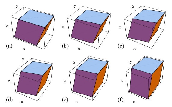
Figure 6: Effect of deformations $\tilde{\underline{\underline{\Lambda}}}^{\prime}$ as given in Eq. (156) for a series of values of $\vartheta$ between (a) $0$ and (f) $\pi/2$ with $\vartheta$ increased in steps of $\pi/10$. In the process a parallelepiped-shaped sample with initial shear in the $xz$-plane is transformed into a parallelepiped with shear in the $yz$-plane that appears as if the original parallelepiped had been rotated by $\pi/2$ about the $z$-axis.

Knowing the deformation tensor $\tilde{\underline{\underline{\Lambda}}}^{\prime}$, we know how the shape of a sample changes in a soft deformation. An equally interesting question is, however, how the orientation of the mesogens changes under such a deformation. To address this question, we recall from Sec. V.1 that rotations in the reference space do not affect the target space vectors such as the director $\bm{{\rm n}}$. Thus, $\bm{{\rm n}}$ does not change in response to rotation described by $O_{R,z}(\vartheta)$. Of course, under target space rotations, $\bm{{\rm n}}$ does change according to $n^{\prime}_{i}=O_{T,ij}n_{j}$. Therefore, the director, as given in Eq. (140), changes in the process of the soft deformation $\tilde{\underline{\underline{\Lambda}}}^{\prime}$ to

$$\bm{{\rm n}}=(\cos\omega\sin\alpha_{T},\sin\omega\sin\alpha_{T},\cos\alpha_{T}).$$ (159)

At this point we pause briefly to compare our findings to AW. Our soft deformation tensor (155) is, up to differences in notation, identical to the soft deformation tensor found by AW, see the last equation in the appendix Ref. adams_warner_SmC_2005 . The same holds true for the change in the director associated with these soft deformations, Eq. (159). However, whereas the AW derivation emphasizes geometric constraints, ours emphasizes that softness arises from invariances with respect to reference space rotations and the independent nature of reference and target space rotations. It should be noted that unlike the AW derivation, ours does not impose incompressibility; rather the incompressibility condition of the soft deformation arises naturally from the from of Eq. (149).

To discuss the implication of the rotational invariance on the Lagrange elastic energy, we now we switch from deformations to strains. In terms of the soft deformation, the general form of the soft strain tensor is given by

$$\underline{\underline{u}}^{\prime}=\textstyle{\frac{1}{2}}\big{[}(\underline{\underline{\Lambda}}^{\prime})^{T}\underline{\underline{\Lambda}}^{\prime}-\underline{\underline{\delta}}\big{]}=\textstyle{\frac{1}{2}}\big{[}(\tilde{\underline{\underline{\Lambda}}}^{\prime})^{T}\tilde{\underline{\underline{\Lambda}}}^{\prime}-\underline{\underline{\delta}}\big{]}\,$$ (160)

independent of target-space rotations. Inserting Eq. (154) or (156), it is straightforward to check that Eq. (160) and Eq. (51a) are equivalent. Using Eq. (154) we find

$$u^{\prime}_{xx}(\vartheta) =-\frac{r_{\perp}-1}{4\,r_{\perp}}\,[1-\cos 2\vartheta]\,,$$ (161a)

$$u^{\prime}_{xy}(\vartheta) =\frac{r_{\perp}-1}{4\,\sqrt{r_{\perp}}}\,\sin 2\vartheta\,,$$ (161b)

$$u^{\prime}_{xz}(\vartheta) =-\frac{s}{r_{\perp}}\,\left[1-(r_{\perp}-1)\cos\vartheta\right]\sin^{2}\frac{\vartheta}{2}\,,$$ (161c)

$$u^{\prime}_{yy}(\vartheta) =\frac{r_{\perp}-1}{4\,r_{\perp}}\,[1-\cos 2\vartheta]\,,$$ (161d)

$$u^{\prime}_{yz}(\vartheta) =\frac{s}{2\,\sqrt{r_{\perp}}}\,\left[r_{\perp}-(r_{\perp}-1)\cos\vartheta\right]\sin\vartheta\,,$$ (161e)

$$u^{\prime}_{zz}(\vartheta) =-\frac{s^{2}}{r_{\perp}}\,\left[1+r_{\perp}-(r_{\perp}-1)\cos\vartheta\right]\sin^{2}\frac{\vartheta}{2}$$ (161f)

for the specifics of the soft strain. Equation (161a) implies that the soft strain has nonzero components for infinitesimal $\vartheta$, viz.

$$u^{\prime}_{xy}(\vartheta) =u^{\prime}_{yx}(\vartheta)=\frac{r_{\perp}-1}{2\,\sqrt{r_{\perp}}}\,\vartheta\,,$$ (162a)

$$u^{\prime}_{yz}(\vartheta) =u^{\prime}_{zy}(\vartheta)=\frac{s}{2\,\sqrt{r_{\perp}}}\,\vartheta\,.$$ (162b)

To ensure that these infinitesimal strains do not cost elastic energy the following combination of elastic constants has to vanish:

$$C_{xyxy}\,(r_{\perp}-1)^{2}+2\,C_{xyyz}\,s(r_{\perp}-1)+C_{yzyz}\,s^{2}=0\,.$$ (163)

This equation is fulfilled if

$$C_{xyxy} =\bar{C}\,\cos^{2}\theta\,,$$ (164a)

$$C_{xyyz} =\bar{C}\,\cos\theta\sin\theta\,,$$ (164b)

$$C_{yzyz} =\bar{C}\,\sin^{2}\theta\,,$$ (164c)

with the angle $\theta$ given by

$$\theta=\tan^{-1}\left(\frac{1-r_{\perp}}{s}\right).$$ (165)

Note by comparing Eqs. (164) and (IV.2) that the analysis of the rotational invariance presented here gives exactly the same relations between the elastic constants as our analyses of the Sm$A$-to-Sm$C$ phase transition presented in Sec. IV and Sec. V.3 to V.4.

Modifying our arguments slightly, we can also understand from them the vanishing of the elastic constants $C_{x^{\prime}y^{\prime}y^{\prime}z^{\prime}}$ and $C_{y^{\prime}z^{\prime}y^{\prime}z^{\prime}}$ in the elastic energy density (IV.2). Rotating the soft strain tensor with the rotation matrix (94) with the rotation angle $\theta$ given by Eq. (165) leads to a soft strain tensor that has in the limit of small $\vartheta$ only

$$u_{y^{\prime}z^{\prime}}(\vartheta) =u_{y^{\prime}z^{\prime}}(\vartheta)=\frac{s}{2\,\sqrt{r_{\perp}}}\,\sqrt{1+\frac{(r_{\perp}-1)^{2}}{s^{2}}}\,\vartheta$$ (166)

as nonzero components. For this strain to cost no energy $C_{x^{\prime}y^{\prime}y^{\prime}z^{\prime}}$ and $C_{y^{\prime}z^{\prime}y^{\prime}z^{\prime}}$ must be zero as they are in Eq. (IV.2).

Next we turn to the question whether extensional strains can be soft in Sm$C$ elastomers. As we did for biaxial smectics we consider extensional strains along the $y$-axis, $u_{yy}^{\prime}>0$, as a specific example. Again we assume, for the sake of the argument, positive anisotropy in the $xy$-plane, $r_{\perp}>1$. Equations (161a) imply that $u_{yy}^{\prime}$ is converted into a zero-energy rotation through an angle $\vartheta$ as given in Eq. (54), if the remaining components relax to

$$u^{\prime}_{xx} =-r_{\perp}^{-1}u^{\prime}_{yy}\,,$$ (167a)

$$u^{\prime}_{xy} =\sqrt{\frac{u^{\prime}_{yy}(r_{\perp}-1-2u^{\prime}_{yy})}{2r_{\perp}}}\,,$$ (167b)

$$u^{\prime}_{xz} =-\frac{s}{2}\,\left[1-\frac{2\,u^{\prime}_{yy}}{r_{\perp}}-\sqrt{1-\frac{2\,u^{\prime}_{yy}}{r_{\perp}-1}}\right],$$ (167c)

$$u^{\prime}_{yz} =\frac{s}{2}\,\sqrt{\frac{2\,u^{\prime}_{yy}}{r_{\perp}\,(r_{\perp}-1)}}$$

$$\times\left[r_{\perp}-\sqrt{(r_{\perp}-1)(r_{\perp}-1-2\,u^{\prime}_{yy})}\right]$$ (167d)

$$u^{\prime}_{zz} =s^{2}\,\left[1-\frac{u^{\prime}_{yy}}{r_{\perp}}-\sqrt{1-\frac{2\,u^{\prime}_{yy}}{r_{\perp}-1}}\right].$$ (167e)

When $u_{yy}^{\prime}$ is increased from zero to $u_{yy}^{\prime}=u_{yy}^{c}\equiv(r_{\perp}-1)/2$, $\vartheta$ grows from zero to $\pi/2$ and the state of the elastomer, originally described by the equilibrium strain tensor $\underline{\underline{u}}^{0}$ is changed without costing elastic energy to

$$\underline{\underline{u}}^{\prime}_{0}=\frac{1}{2}\left(\begin{array}[]{ccc}r_{\perp}^{-1}-1&0&-s/r_{\perp}\\ 0&r_{\perp}-1&s\sqrt{r_{\perp}}\\ -s/r_{\perp}&s\sqrt{r_{\perp}}&s^{2}(r_{\perp}^{-1}+1)\end{array}\right),$$ (171)

which is, of course, the strain tensor associated with the deformation tensor of Eq. (157).

In this process, the shape of the sample changes as depicted in Fig. 6. As already discussed, the configuration at $\vartheta=\pi/2$ describes a sample in which the Sm$A$ phase was sheared in the $yz$- rather than the $xz$ plane. Thus further increase in $u^{\prime}_{yy}$ beyond $u_{yy}^{c}$ is equivalent to increasing $u^{\prime}_{xx}$ beyond zero in the original sample sheared in the $xz$-plane. Thus, the second Piola-Kirchhoff stress is

$$\sigma^{\text{II}}_{yy}=\begin{cases}0&\text{if $u_{yy}^{\prime}<u_{yy}^{c}$},\\ Y_{x}\,(u_{yy}^{\prime}-u_{yy}^{c})&\text{if $u_{yy}^{\prime}>u_{yy}^{c}$},\cr\end{cases}$$ (172)

where $Y_{x}$ is the Youngs modulus for stretching along $x$. Equation (172) implies that the stress usually measured in experiments, i.e. the engineering stress, is given at leading order by

$$\sigma^{\text{eng}}_{yy}=\begin{cases}0&\text{if $\tilde{\Lambda}^{\prime}_{yy}<\sqrt{r_{\perp}}$},\\ Y_{x}\,\tilde{\Lambda}^{\prime}_{0yy}\,(\tilde{\Lambda}^{\prime}_{yy}-\tilde{\Lambda}^{\prime}_{0yy})&\text{if $\tilde{\Lambda}^{\prime}_{yy}>\sqrt{r_{\perp}}$}.\cr\end{cases}$$ (173)

Therefore, when plotted as a function of the deformation $\tilde{\Lambda}^{\prime}_{yy}$, the engineering stress $\sigma^{\text{eng}}_{yy}$ for a Sm$C$ elastomer looks qualitatively the same as the corresponding curve for a nematic or a biaxial smectic elastomer, cf. Fig. 3.

VI Concluding remarks

In summary, we have presented models for transitions from uniaxial Sm$A$ elastomers to biaxial and Sm$C$ elastomers: Landau-like phenomenological models as functions of the Cauchy–Saint-Laurent strain tensor for both the transitions as well as a detailed model for the transition from the Sm$A$ to the smectic-$C$ phase. The detailed model includes contributions from the elastic network, smectic layer compression, and coupling of the Frank director to the smectic layer normal, and allowed for estimating the magnitudes of its phenomenological coupling constants. We employed the three models to investigate the nature of the soft elasticity, required by symmetry, of monodomain samples of the biaxial and Sm$C$ phases.

We learned that biaxial smectic elastomers are soft with respect to shears in the smectic plane. In addition to that we saw that extensional strains can be converted by the material into zero-energy rotations, provided the experimental boundary conditions are not too restrictive and allow the remaining strain degrees of freedom to relax. We illustrated this softness by explicitly considering an elongation in the $y$ direction (the direction perpendicular to the order in the smectic plane) as a specific example. However, we could impose an extensional strain in any direction and we would find softness, provided the c-director has freedom to rotate into that direction. This excludes only stretches in directions lying in the plane spanned by the equilibrium c-director and the initial uniaxial direction (i.e., in our convention stretches in directions lying in the $xz$-plane). Of course, the width of the soft plateau in the stress-strain curve, c.f. Fig. 3, depends on how much the c-director can rotate until it has reached the direction of a stretch. Therefore, the soft plateau will be most pronounced for stretches perpendicular to the plane spanned by the equilibrium c-director and the initial uniaxial direction (our $y$-direction).

The softness of Sm$C$ elastomers is more intricate than that of biaxial smectics. At first sight it seems as if it takes a very specific combination of shears to achieve a soft response. However, with the coordinate system chosen appropriately, it turns out that Sm$C$ elastomers are soft with respect to certain conventional shear strains (with our conventions shears in the $y^{\prime}z^{\prime}$-plane). Even more important, as far as possible experimental realizations of softness Sm$C$ elastomers are concerned, is that these materials are also soft under extensional strains. What we have said above for biaxial smectics also applies here: the experimental boundary conditions must be right and the direction of the imposed stretch must be so that the c-director can rotate.

As pointed out in the introduction, very recently considerable experimental progress was made by Hiraoka et al. hiraoka&CO_2005 , who synthesized a monodomain sample of a Sm$C$ elastomer forming spontaneously from a Sm$A$ phase upon cooling. This is exactly the type of elastomer for which our Sm$C$ theory was made. Therefore, it seems well founded to hope that our predictions for Sm$C$ elastomers can be tested experimentally in the near future.

Appendix A Effects of higher orders in the strains

A priori, a formulation of stretching energy densities in terms of the variables $\eta$ and $\eta_{z}$ provides a more adequate framework for discussing the incompressible limit than a formulation in terms of the respective linearized expressions $u_{ii}$ and $u_{zz}$. Using $u_{ii}$ and $u_{zz}$, on the other hand, makes our models more tractable and perhaps also more intuitive because we stay in close contact to the standard formulation of elasticity as presented in textbooks. The purpose of this appendix is to discuss what changes occur in our theories if we use $\eta$ and $\eta_{z}$ instead of $u_{ii}$ and $u_{zz}$.

A.1 Biaxial elastomers

Now we use Eq. (II) as the starting point for setting up our model for soft biaxial elastomers. When $C_{4}$ can become negative, higher order terms featuring $\hat{u}_{ab}$, $\eta$ and $\eta_{z}$ must be added to Eq. (II) so that the model elastic energy density becomes

$$f_{\text{uni}}^{(2)}=f_{\text{uni}}+A_{1}\,\eta_{z}\,\hat{u}_{ab}^{2}+A_{2}\,\eta\,\hat{u}_{ab}^{2}+B\,(\hat{u}_{ab}^{2})^{2}\,.$$ (174)

Proceeding in close analogy to the steps described following Eq. (16), we find that the equilibrium values of $\eta$ and $\eta_{z}$ are

$$\eta_{z}^{0} =\alpha\,(\hat{u}_{ab}^{0})^{2}=\textstyle{\frac{1}{2}}\,\alpha\,S^{2}\,,$$ (175a)

$$\eta^{0} =\beta\,(\hat{u}_{ab}^{0})^{2}=\textstyle{\frac{1}{2}}\,\beta\,S^{2}\,,$$ (175b)

with $\alpha$ and $\beta$ as given in Eq. Eq. (24). The equilibrium values $u^{0}_{az}$ and $\hat{u}_{ab}^{0}$ remain unchanged. To learn more about the equilibrium state, our next task is to determine the equilibrium strain tensor $\underline{\underline{u}}^{0}$. Using our knowledge about $u^{0}_{az}$ and $\hat{u}_{ab}^{0}$, it is clear that $\underline{\underline{u}}^{0}$ is of the form

$$\underline{\underline{u}}^{0}=\left(\begin{array}[]{ccc}\frac{1}{2}(t+S)&0&0\\ 0&\frac{1}{2}(t-S)&0\\ 0&0&u_{zz}^{0}\end{array}\right),$$ (179)

where we used the abbreviation $t=u_{cc}^{0}$. $t$ and $u_{zz}^{0}$ are unknown thus far and we need to determine them as functions of the order parameter $S$. Replacing $\eta_{z}$ and $u_{zz}$ in Eq. (11b) by $\eta_{z}^{0}$ and $u_{zz}^{0}$, using Eq. (175a) for $\eta_{z}^{0}$ and solving for $u_{zz}^{0}$ we find

$$u_{zz}^{0}=\frac{1}{2}\,\left[\left(1+\textstyle{\frac{1}{2}}\,\alpha\,S^{2}\right)^{2}-1\right].$$ (180)

To leading order in $S$ this result reduces to $u_{zz}^{0}=\textstyle{\frac{1}{2}}\,\alpha\,S^{2}$ which coincides with the result of our linearized theory presented in Sec. III. It remains to calculate $t$. Since $\underline{\underline{u}}^{0}$ is diagonal, Eq. (11a) leads simply to

$$\eta^{0}=\left[(1+t+S)(1+t-S)(1+2u_{zz}^{0})\right]^{1/2}-1\,.$$ (181)

Using Eqs. (175) for $\eta^{0}$ and $u_{zz}^{0}$ we obtain by solving for $t$:

$$t=\left[\frac{(1+\frac{\beta}{2}\,S^{2})^{2}}{(1+\frac{\alpha}{2}\,S^{2})^{2}}+S^{2}\right]^{1/2}-1\,.$$ (182)

To leading order in $S$ this expression reduces to $t=\frac{1}{2}(\beta-\alpha+1)S^{2}$. Comparing this to the result $u_{cc}^{0}=\frac{1}{2}(\beta-\alpha)S^{2}$ of our linearized theory, we see that the linearized theory lacks the contribution $\frac{1}{2}S^{2}$ to $u_{cc}^{0}$. Nevertheless, up to this detail, the form of the equilibrium state predicted by the linearized and the non-linearized theory is the same. In the end, the non-linearized theory leads to the elastic energy density

$$f= \textstyle{\frac{1}{2}}C_{1}g_{zz}^{-2}(\delta u_{zz})^{2}+C_{2}g_{zz}^{-1}\overline{u}\delta u_{zz}+\textstyle{\frac{1}{2}}C_{3}(\overline{u})^{2}$$

$$+C_{5}(\delta u_{az})^{2}+B_{2}S^{2}(\delta u_{xx}-\delta u_{yy})^{2}$$

$$+(A_{1}Sg_{zz}^{-1/2}\delta u_{zz}+A_{2}S\overline{u})(\delta u_{xx}-\delta u_{yy}),$$ (183)

for the soft biaxial state, where

$$\overline{u}=[\det(1+2\underline{\underline{u}}_{0})]^{1/2}\,\,[(\underline{\underline{\delta}}+2\underline{\underline{u}}_{0})^{-1}\delta\underline{\underline{u}}]_{ii}=\frac{V_{B}}{V_{0}}u^{\prime}_{ii}\approx\frac{\delta V}{V_{0}},$$ (184)

where $V_{0}$ is the volume of the reference uniaxial state, $V_{B}$ is the volume of the biaxial state and $\delta V=V-V_{B}$. Thus, volume changes in the biaxial phase are suppressed by the term proportional to $C_{3}$ in Eq. (183). In the incompressible limit $C_{3}\rightarrow\infty$, the nonlinear theory indeed produces fixed $\delta V=0$ and not $\delta u_{ii}=0$ as the linearized theory does. Our findings about the softness of the biaxial state, however, remain practically the same.

A.2 Sm$C$-elastomers

When $C_{5}$ can become negative in response to Sm$C$ ordering of the mesogens, higher order terms featuring $u_{az}$, $\eta$ and $\eta_{z}$ must be added to Eq. (II) to ensure mechanical stability. Then the model elastic energy density becomes

$$f_{\text{uni}}^{(2)} =f_{\text{uni}}+D_{1}\,\eta_{z}\,u_{az}^{2}+D_{2}\,\eta\,u_{az}^{2}+D_{3}\,\hat{u}_{ab}u_{az}u_{bz}$$

$$+E\,(u_{az}^{2})^{2}\,.$$ (185)

Essentially repeating the algebra described following Eq. (IV.1), we find

$$\eta_{z}^{0} =\sigma\,(u_{az}^{0})^{2}=\sigma\,S^{2}\,,$$ (186a)

$$\eta^{0} =\tau\,(u_{az}^{0})^{2}=\tau\,S^{2}\,,$$ (186b)

with $\sigma$ and $\tau$ as given in Eq. (73). $\hat{u}_{ab}^{0}$ and $u_{az}^{0}$ remain the same as in Sec. IV.1. Consequently, the equilibrium strain tensor is of the form

$$\underline{\underline{u}}^{0}=\left(\begin{array}[]{ccc}\frac{t}{2}&0&S\\ 0&\frac{t}{2}&0\\ S&0&u_{zz}^{0}\end{array}\right),$$ (190)

where $t=u_{cc}^{0}$. For determining the equilibrium state, it remains to compute $t$ and $u_{zz}^{0}$ as functions of $S$. From Eqs. (11b) and (186a) it follows readily that

$$u_{zz}^{0}=\frac{1}{2}\,\left[\left(1+\sigma\,S^{2}\right)^{2}-1\right],$$ (191)

which is to leading order in $S$ identical to the result $u_{zz}^{0}=\sigma\,S^{2}$ of our linearized theories for Sm$C$ elastomers. Equations (11b) and (190) lead us to

$$\eta^{0}=\left[(1+t)^{2}(1+2\,u_{zz}^{0})-4\,(1+t)S^{2}\right]^{1/2}-1\,.$$ (192)

Taking into account the equilibrium values (186a) and solving for $t$ we find

$$t=\frac{2S^{2}}{(1+\sigma S^{2})^{2}}+\left[\frac{(1+\tau S^{2})^{2}}{(1+\sigma S^{2})^{2}}+\frac{4S^{4}}{(1+\sigma S^{2})^{4}}\right]^{1/2}-1\,.$$ (193)

To leading order in $S$, $t=(\tau-\sigma+2)\,S^{2}$ which has to be compared to the $u_{cc}^{0}=(\tau-\sigma)\,S^{2}$ stemming from our linearized theories for Sm$C$ elastomers. Note that the linearized theories miss the contribution $2S^{2}$ to $u_{cc}^{0}$. However, as was the case for the biaxial soft state, this discrepancy does not affect the nature of the softness.

Appendix B Elastic constants

This appendix collects our results for the elastic constants of biaxial and Sm$C$ elastomers.

B.1 Elastic constants of biaxial elastomers

The elastic constants of soft biaxial elastomers as defined in the elastic energy density (III.2) are given to order $O(S^{3})$ by

$$C_{zzzz} =C_{1}+2C_{2}+C_{3}+2\alpha[C_{1}+2C_{2}+C_{3}]\,S^{2}\,,$$ (194)

$$C_{xzxz} =2[C_{5}+C_{5}\,S+\textstyle{\frac{1}{2}}(\alpha+\beta)C_{5}\,S^{2}]\,,$$ (195)

$$C_{yzyz} =2[C_{5}-C_{5}\,S+\textstyle{\frac{1}{2}}(\alpha+\beta)C_{5}\,S^{2}]\,,$$ (196)

$$C_{zzxx} =C_{2}+C_{3}+[C_{2}+C_{3}+A_{1}+A_{2}]\,S$$

$$+[\textstyle{\frac{1}{2}}(\alpha+\beta)(C_{2}+C_{3})+A_{1}+A_{2}]\,S^{2}\,,$$ (197)

$$C_{zzyy} =C_{2}+C_{3}-[C_{2}+C_{3}+A_{1}+A_{2}]\,S$$

$$+[\textstyle{\frac{1}{2}}(\alpha+\beta)(C_{2}+C_{3})+A_{1}+A_{2}]\,S^{2}\,,$$ (198)

$$C_{xxxx} =C_{3}+2[C_{3}+A_{2}]\,S$$

$$+[(1-\alpha+\beta)C_{3}+4A_{2}+2B]\,S^{2}\,,$$ (199)

$$C_{yyyy} =C_{3}-2[C_{3}+A_{2}]\,S$$

$$+[(1-\alpha+\beta)C_{3}+4A_{2}+2B]\,S^{2}\,,$$ (200)

$$C_{xxyy} =C_{3}-[(1+\alpha-\beta)C_{3}+2B]\,S^{2}\,.$$ (201)

B.2 Elastic constants of Sm$C$ elastomers

Here we list our results for the elastic constants of soft Sm$C$ elastomers as defined in Eq. (IV.2).

B.2.1 Elastic constants as obtained from the strain-only model of Sec. IV

Our results for the angle $\theta$ and the elastic constant $\bar{C}$ read

$$\theta =\tan^{-1}\left(\frac{-\Lambda_{zz}^{0}\omega\,S}{\Lambda_{xx}^{0}-\Lambda_{xz}^{0}\omega\,S}\right)=-\omega\,S+O(S^{3})\,,$$ (202)

$$\bar{C} =4C_{4}\,\frac{(\Lambda_{yy}^{0})^{2}(\Lambda_{xx}^{0}-\Lambda_{xz}^{0}\omega\,S)^{2}}{\cos^{2}\theta}$$

$$=4C_{4}+4C_{4}[2(\tau-\sigma)+(\omega-4)\omega]\,S^{2}+O(S^{4})\,.$$ (203)

For the remaining elastic constants we find to order $O(S^{3})$

$$C_{zzzz} =C_{1}+2C_{2}+C_{3}+4(\sigma-2)(C_{1}+2C_{2}+C_{3})\,S^{2}\,,$$ (204)

$$C_{xzxz} =8[2(C_{1}+2C_{2}+C_{3})+2(D_{1}+D_{2})+E]\,S^{2}\,,$$ (205)

$$C_{zzxx} =C_{2}+C_{3}+[(\sigma+\tau+\omega-4)(C_{2}+C_{3})$$

$$+4(C_{1}+2C_{2}+C_{3})+4(D_{1}+D_{2})]\,S^{2}\,,$$ (206)

$$C_{zzyy} =C_{2}+C_{3}+(\sigma+\tau-\omega-4)(C_{2}+C_{3})\,S^{2}\,,$$ (207)

$$C_{xxxx} =C_{3}+C_{4}+2[4C_{2}+(4+\tau+\omega-\sigma)C_{3}$$

$$+(\tau+\omega-\sigma)C_{4}+2(2D_{2}+D_{3})]\,S^{2}\,,$$ (208)

$$C_{yyyy} =C_{3}+C_{4}+2(\tau-\omega-\sigma)(C_{3}+C_{4})\,S^{2}\,,$$ (209)

$$C_{xxyy} =C_{3}-C_{4}+2[2(C_{2}+C_{3})-(\sigma-\tau)(C_{3}-C_{4})$$

$$+2D_{2}-D_{3}]\,S^{2}\,,$$ (210)

$$C_{xxxz} =[4(C_{2}+C_{3})+2D_{2}+D_{3}]\,S\,,$$ (211)

$$C_{yyxz} =[4(C_{2}+C_{3})+2D_{2}-D_{3}]\,S\,,$$ (212)

$$C_{zzxz} =2[2(C_{1}+2C_{2}+C_{3})+D_{1}+D_{2}]\,S\,.$$ (213)

B.2.2 Elastic constants as obtained from the model with strain and director of Sec. V

For $\theta$ and $\bar{C}$ we find

$$\theta =\tan^{-1}\left(\frac{-\Lambda_{zz}^{0}\,\Pi}{\Lambda_{xx}^{0}\,\Xi-\Lambda_{xz}^{0}\,\Pi}\right)=-\frac{\bar{\omega}}{\bar{\rho}}\,S+O(S^{3})\,,$$ (214)

$$\bar{C} =4\,\frac{C_{4}C_{5}}{\Delta}\,\frac{(\Lambda_{yy}^{0})^{2}\,(\Lambda_{xx}^{0}\,\Xi-\Lambda_{xz}^{0}\,\Pi)^{2}}{\cos^{2}\theta}$$

$$=4C_{4}+4\frac{2\bar{\omega}^{2}C_{4}+[2\bar{\rho}^{2}(\bar{\sigma}-\bar{\tau}+2\bar{\omega})-\bar{\omega}^{2}]C_{5}}{\bar{\rho}^{2}\,C_{5}}\,C_{4}\,S^{2}$$

$$+O(S^{4})\,.$$ (215)

The remaining elastic constants are given to order $O(S^{3})$ by

$$C_{zzzz} =C_{1}+2C_{2}+C_{3}+4\bigg{[}(\bar{\sigma}-2\bar{\rho}^{2})$$

$$\times(C_{1}+2C_{2}+C_{3})-2\frac{(\lambda_{1}+\lambda_{2})^{2}}{\lambda_{4}^{2}}C_{5}\bigg{]}\,S^{2}\,,$$ (216)

$$C_{xzxz} =8\bigg{[}2\bar{\rho}^{2}(C_{1}+2C_{2}+C_{3})$$

$$+\frac{gC_{5}+\lambda_{4}[\lambda_{4}-2(2\lambda_{2}-\lambda_{3})]}{\lambda_{4}^{2}}C_{5}\bigg{]}\,S^{2}\,,$$ (217)

$$C_{zzxx} =C_{2}+C_{3}+\bigg{[}4\bar{\rho}^{2}C_{1}+(4\bar{\rho}^{2}+\bar{\sigma}+\bar{\tau}+\bar{\omega})C_{2}$$

$$+(\bar{\sigma}+\bar{\tau}+\bar{\omega})C_{3}-4\frac{2\lambda_{2}^{2}+\lambda_{1}(2\lambda_{2}+\lambda_{3})}{\lambda_{4}^{2}}C_{5}$$

$$+4\frac{\bar{\rho}\lambda_{3}\lambda_{4}-\lambda_{2}(\lambda_{3}+2\bar{\rho}\lambda_{4})}{\lambda_{4}^{2}}C_{5}\bigg{]}\,S^{2},$$ (218)

$$C_{zzyy} =C_{2}+C_{3}+\bigg{[}(\bar{\sigma}+\bar{\tau}-\bar{\omega}-4\bar{\rho}^{2})(C_{2}+C_{3})$$

$$-4\frac{(\lambda_{1}+\lambda_{2})(2\lambda_{2}-\lambda_{3})}{\lambda_{4}^{2}}C_{5}\bigg{]}\,S^{2}\,,$$ (219)

$$C_{xxxx} =C_{3}+C_{4}+2\bigg{[}4\bar{\rho}^{2}(C_{2}+C_{3})$$

$$+(\bar{\tau}+\bar{\omega}-\bar{\sigma})(C_{3}+C_{4})$$

$$-\frac{(2\lambda_{2}+\lambda_{3})^{2}+8\bar{\rho}\lambda_{4}(\lambda_{1}+\lambda_{2})}{\lambda_{4}^{2}}C_{5}\bigg{]}S^{2}\,,$$ (220)

$$C_{yyyy} =C_{3}+C_{4}+2\bigg{[}(\bar{\tau}-\bar{\omega}-\bar{\sigma})(C_{3}+C_{4})$$

$$+\frac{(2\lambda_{2}-\lambda_{3})^{2}}{\lambda_{4}^{2}}C_{5}\bigg{]}\,S^{2}\,,$$ (221)

$$C_{xxyy} =C_{3}-C_{4}+2\bigg{[}2\bar{\rho}^{2}(C_{2}+C_{3})-(\bar{\sigma}-\bar{\tau})(C_{3}-C_{4})$$

$$-2\frac{(\lambda_{1}+\lambda_{2})(2\lambda_{2}-\lambda_{3})+\bar{\rho}\lambda_{4}(2\lambda_{2}+\lambda_{3})}{\lambda_{4}^{2}}C_{5}\bigg{]}\,S^{2}\,,$$ (222)

$$C_{xxxz} =4\bigg{[}\bar{\rho}(C_{2}+C_{3})-\frac{\lambda_{1}+\lambda_{2}}{\lambda_{4}}C_{5}\bigg{]}\,S\,,$$ (223)

$$C_{yyxz} =2\bigg{[}2\bar{\rho}(C_{2}+C_{3})-\frac{2\lambda_{2}+\lambda_{3}}{\lambda_{4}}C_{5}\bigg{]}\,S\,,$$ (224)

$$C_{zzxz} =2\bigg{[}2\bar{\rho}(C_{1}+2C_{2}+C_{3})-\frac{2\lambda_{2}-\lambda_{3}}{\lambda_{4}}C_{5}\bigg{]}\,S\,.$$ (225)

Appendix C Steps leading to Eq. (V.4)

In this appendix we outline some of the algebraic steps leading from Eqs. (V.4) and (143) to Eq. (V.4). As discussed in the text following Eq. (122), the role of $\delta\tilde{c}_{y}$ is special in that it is the local relaxation of this quantity that makes Sm$C$ elastomers soft. To see this, we recast Eq. (V.4), where $\delta\tilde{c}_{y}$ appears in two different terms, by using

$$2C_{4}\left(\delta\bar{w}_{xy}\right)^{2}+C_{5}\left(\delta\bar{w}_{yz}\right)^{2}$$

$$=\Delta\left[\delta\tilde{c}_{y}+\frac{2C_{4}\,\Pi\,\delta u_{xy}+C_{5}\,\Xi\,\delta u_{yz}}{\Delta}\right]^{2}$$

$$+2\,\frac{C_{4}C_{5}}{\Delta}\,\left[\Pi\,\delta u_{yz}-\Xi\,\delta u_{xy}\right]^{2},$$ (226)

with $\Pi$, $\Xi$, and $\Delta$ as defined below Eq. (V.4). The validity of Eq. (C) can be checked by straightforward but slightly tedious algebra.

The second major step in going from Eqs. (V.4) and (143), after these are combined, to Eq. (V.4) is to integrate out the massive variable $\delta\tilde{c}_{x}$, i.e., to replace $\delta\tilde{c}_{x}$ by its minimum value. This minimization is straightforward but a little inconvenient because of the number of terms that are involved. Combining Eq. (C) and the outcome of this minimization we arrive at the intermediate result

$$\delta f =\Delta\left[\delta\tilde{c}_{y}+\frac{2C_{4}\,\Pi\,\delta u_{xy}+C_{5}\,\Xi\,\delta u_{yz}}{\Delta}\right]^{2}+2\,\frac{C_{4}C_{5}}{\Delta}\,\left[\Pi\,\delta u_{yz}-\Xi\,\delta u_{xy}\right]^{2}$$

$$+\frac{1}{2}\bigg{[}C_{1}+2C_{2}+C_{3}-\frac{2}{\Omega}(\lambda_{1}+\lambda_{2})^{2}S^{2}\bigg{]}(\delta u_{zz})^{2}+\bigg{[}C_{5}-\frac{\lambda_{4}^{2}}{4\Omega}\left(1-\frac{3}{2}S^{2}\right)\bigg{]}(\delta u_{xz})^{2}$$

$$+\frac{1}{2}\bigg{[}C_{3}+C_{4}-\frac{2}{\Omega}\left(\lambda_{2}+\frac{\lambda_{3}}{2}\right)^{2}S^{2}\bigg{]}(\delta u_{xx})^{2}+\frac{1}{2}\bigg{[}C_{3}+C_{4}+\frac{2}{\Omega}\left(\lambda_{2}-\frac{\lambda_{3}}{2}\right)^{2}S^{2}\bigg{]}(\delta u_{yy})^{2}$$

$$+\bigg{[}C_{2}+C_{3}-\frac{2}{\Omega}(\lambda_{1}+\lambda_{2})\left(\lambda_{2}+\frac{\lambda_{3}}{2}\right)S^{2}\bigg{]}\delta u_{zz}\delta u_{xx}+\bigg{[}C_{2}+C_{3}-\frac{2}{\Omega}(\lambda_{1}+\lambda_{2})\left(\lambda_{2}-\frac{\lambda_{3}}{2}\right)S^{2}\bigg{]}\delta u_{zz}\delta u_{yy}$$

$$+\bigg{[}C_{3}-C_{4}-\frac{2}{\Omega}(\lambda_{1}+\lambda_{2})\left(\lambda_{2}-\frac{\lambda_{3}}{2}\right)S^{2}\bigg{]}\delta u_{xx}\delta u_{yy}+\bigg{[}-\frac{1}{\Omega}(\lambda_{1}+\lambda_{2})\lambda_{4}\,S\left(1-\frac{3}{2}S^{2}\right)\bigg{]}\delta u_{xx}\delta u_{xz}$$

$$+\bigg{[}-\frac{1}{\Omega}\left(\lambda_{2}+\frac{\lambda_{3}}{2}\right)\lambda_{4}\,S\left(1-\frac{3}{2}S^{2}\right)\bigg{]}\delta u_{yy}\delta u_{xz}+\bigg{[}-\frac{1}{\Omega}\left(\lambda_{2}-\frac{\lambda_{3}}{2}\right)\lambda_{4}\,S\left(1-\frac{3}{2}S^{2}\right)\bigg{]}\delta u_{zz}\delta u_{xz}\,,$$ (227)

where we have used the shorthand $\Omega=gS^{2}+C_{5}\bar{\rho}^{2}(1+5S^{2}/2)$. Switching from the strain variable $\delta\underline{\underline{u}}$ to $\underline{\underline{u}}^{\prime}=(\underline{\underline{\Lambda}}^{0T})^{-1}\delta\underline{\underline{u}}\,(\underline{\underline{\Lambda}}^{0})^{-1}$ then takes us to Eq. (V.4).

Appendix D Effects of the Frank energy on the softness

In Sec. V we have neglected the Frank energy. In this appendix we check if our conclusions about the softness of Sm$C$ elastomers are affected if we take the Frank energy, or rather the corresponding density

$$f_{\text{Frank}} =\textstyle{\frac{1}{2}}K_{1}\,[\nabla\cdot\bm{{\rm n}}]^{2}+\textstyle{\frac{1}{2}}K_{2}\,[\bm{{\rm n}}\cdot(\nabla\times\bm{{\rm n}})]^{2}$$

$$+\textstyle{\frac{1}{2}}K_{3}\,[\bm{{\rm n}}\times(\nabla\times\bm{{\rm n}})]^{2},$$ (228)

into account. To this end we have to check if Eq. (D) can lead to a mass for $\delta\tilde{c}_{y}$.

Each of the three terms in Eq. (D) features a derivative. Since the director $\bm{{\rm n}}$ lives in the target space, these derivatives are derivatives with respect to the target space coordinate $\bm{{\rm R}}$, i.e.,

$$\nabla_{k}n_{i}=\frac{\partial n_{i}}{\partial R_{k}}=\big{(}\underline{\underline{\Lambda}}^{-1}\big{)}_{lk}\frac{\partial n_{i}}{\partial x_{l}}\,.$$ (229)

In Sec. V we modeled Sm$C$ elastomers via converting the director to a reference space vector by using the polar decomposition theorem. Doing the same conversion here we get with the help of Eq. (99)

$$\nabla_{k}n_{i}=\big{(}\underline{\underline{\Lambda}}^{-1}\big{)}_{lk}\left\{\frac{\partial O_{ij}}{\partial x_{l}}\,\tilde{n}_{j}+O_{ij}\,\frac{\partial\tilde{n}_{j}}{\partial x_{l}}\right\}\,.$$ (230)

The second term in the braces contains a derivative of $\tilde{n}_{j}$ and hence it is clear that it cannot lead to a massive term. This leaves us with the first term in the braces as a potential source of a mass. Using Eq. (98) we get

$$\frac{\partial O_{ij}}{\partial x_{l}}=\frac{\partial}{\partial x_{l}}\,\eta_{Aij}+\cdots\,,$$ (231)

where $\eta_{Aij}=\frac{1}{2}(\partial_{j}u_{i}-\partial_{i}u_{j})$ is the antisymmetric part of the displacement gradient tensor $\eta_{ij}=\partial_{j}u_{i}$. Thus, the first term in the braces couples $\tilde{n}_{j}$ to derivatives of $\eta_{ij}$ and higher order terms, and as such this term cannot make $\delta\tilde{c}_{y}$ massive in a perturbative (diagrammatic) expansion. Furthermore, the terms in this expansion will be subdominant compared to the $u_{yz}{\tilde{c}}_{y}$ at small wavenumber $q$. Rotational invariance in the reference space should dictate that Frank energy terms do not ever generate a mass for ${\tilde{c}}_{y}$, a full demonstration of this fact to all orders in perturbation theory is beyond the scope of this paper. We conclude that our findings about the soft elasticity of Sm$C$ elastomers remain unchanged if we include the Frank energy in our model.

References

- (1) For a review on liquid crystal elastomers see W. Warner and E.M. Terentjev, Liquid Crystal Elastomers (Clarendon Press, Oxford, 2003)
- (2) For a review on liquid crystals see P. G. de Gennes and J. Prost, The Physics of Liquid Crystals (Clarendon Press, Oxford, 1993); S. Chandrasekhar, Liquid Crystals (Cambridge University Press, Cambridge, 1992).
- (3) L. Golubović and T. C. Lubensky, Phys. Rev. Lett. 63, 1082 (1989).
- (4) H. Finkelmann, I. Kundler, E. M. Terentjev, and M. Warner, J. Phys. II (France) 7, 1059 (1997).
- (5) G. C. Verwey, M. Warner, and E. M. Terentjev, J. Phys. II (France) 6, 1273 (1996).
- (6) M. Warner, J. Mech. Phys. Solids 47, 1355 (1999).
- (7) T. C. Lubensky, R. Mukhopadhyay, L. Radzihovsky, and X.J. Xing, Phys. Rev. E 66, 011702 (2002).
- (8) E. M. Terentjev, I. V. Kamotski, D. D. Zakharov, and L. J. Fradkin, Phys. Rev. E 66, 052701(R) (2002). L. J. Fradkin, I. V. Kamotski, E. M. Terentjev and D. D. Zakharov, Proc. R. Soc. Lond. A 459, 2627 (2003).
- (9) O. Stenull and T. C. Lubensky, Phys. Rev. E 69, 051801 (2004).
- (10) O. Stenull and T. C. Lubensky, Eur. Phys. J. E 14, 333 (2004).
- (11) O. Stenull and T. C. Lubensky, Eurohys. Lett. 61, 776 (2003). See also, X. Xing and L. Radzihovsky, Eurohys. Lett. 61, 769 (2003).
- (12) O. Stenull and T. C. Lubensky, Phys. Rev. E 69, 021807 (2004).
- (13) X. Xing and L. Radzihovsky, Phys. Rev. Lett. 90, 168301 (2003).
- (14) V. P. Shibaev, H. Finkelmann, A. V. Kharitonov, M. Portugal, N. A. Plate, and H. Ringsdorf, Vysokomol. Soed. A 23, 919 (1981); V. P. Shibaev, S. G. Kostromin, and N. A. Plate, Euro. Polym. J. 18, 651 (1982).
- (15) P. Fischer, C. Schmidt, and H. Finkelmann, Macromol. Rapid Comm. 16, 435 (1995).
- (16) M. Bremer et al., Polymer Preprints 34, 708 (1993); M. Bremer et al., Macromol. Chem. Phys. 195, 1891 (1994).
- (17) I. Benne, K. Semmler, and H. Finkelmann, Macromol. Chem. Rapid Commun. 15, 295 (1994).
- (18) K. Hiraoka and H. Finkelmann, Macromol. Chem. Rapid Commun. 22, 456 (2001).
- (19) K. Hiraoka, W. Sagano, T. Nose and H. Finkelmann, Macromolocules 38, 7352 (2005).
- (20) E. Gebhard and R. Zentel, Macromolecular Rapid Communications 10, 341(1998).
- (21) R. Zentel, E. Gebhard, M. Brehmer, Advances in Liquid Crystals, Advances in Chemical Physics, edited by J. K. Vij, I. Prigogine, S. A. Rice (John Viley and Sons, New York, 2000) 113, 159.
- (22) R. Stannarius, R. Kohler, U. Dietrich, M. Losche, C. Tolksdorf, and R. Zentel. Phys.Rev. E, 65, 041707 (2002).
- (23) W. Lehmann et al., Nature 410, 447 (2001).
- (24) R. B. Meyer, L. Liebert, L. Strzelecki, and P. Keller, J. de Phys. Lett. 36, L68 (1975).
- (25) E. M. Terentjev and M. Warner, J. Phys. II (France) 4, 111 (1994).
- (26) E. M. Terentjev and M. Warner, J. Phys. II (France) 4, 849 (1994).
- (27) T. C. Lubensky, E. M. Terentjev, and M. Warner, J. Phys. II (France) 4, 1457 (1994).
- (28) E. M. Terentjev, M. Warner, and T. C. Lubensky, Europhys. Lett. 30, 343 (1995).
- (29) J. Weilepp and H. R. Brand, Macromol. Theory Simul. 7, 91 (1998).
- (30) M. J. Osborne and E. M. Terentjev, Phys. Rev. E 62, 5101 (2000).
- (31) J. M. Adams and M. Warner, Phys. Rev. E 71, 021708 (2005).
- (32) J. M. Adams and M. Warner, Phys. Rev. E 72, 011703 (2005).
- (33) J.M. Adams and M. Warner, Phys. Rev. E 73, 031706 (2006)
- (34) O. Stenull and T. C. Lubensky, Phys. Rev. E 73, 030701(R) (2006); O. Stenull and T. C. Lubensky forthcoming paper.
- (35) L. Radzihovsky and J. Toner, Phys. Rev. B 60, 206 (1999).
- (36) O. Stenull and T. C. Lubensky, forthcoming paper.
- (37) O. Stenull and T. C. Lubensky, Phys. Rev. Lett. 94, 018304 (2005).
- (38) L. D. Landau and E. M. Lifshitz, Theory of Elasticity, 3rd Edition (Pergamon Press, New York, 1986).
- (39) P. M. Chaikin and T. C. Lubensky, Principles of Condensed Matter Physics (Cambridge Press, Cambridge, 1995).
- (40) If were a standard vector field transforming under the same operators as , then would equal . We have chosen to work with rather than so that, in this case, the transformation looks like the standard transformation of fields that transform under the same group as space points. See, e.g., M. Peskin and D. Schroeder, An Introduction to Quantum Field Theory (Perseus Books, Reading, MA, 1995).
- (41) The vector is in most cases identical to the director specifying the direction of nematic order in the notation of the text by Warner and Terentjev WarnerTer2003 . contracts only with the right index of , whereas the Frank director is a target space vector that contracts only with its left index. Thus, invariants of the form are permitted.
- (42) A. Love, A Treatise on the Mathematical Theory of Elasticity (Dover Publications, New York, 1944).
- (43) The stress tensor defined in Eq. (46) is the second Piola-Kirchhoff stress tensor. It transforms like a tensor in the reference space but like a scalar under rotations in the target space. The more familiar Cauchy stress tensor, which transforms like a tensor in the target space is . The engineering or first Piola-Kirchhoff stress tensor, , is a mixed tensor that transform like a vector under rotations in either the reference or the targt space.
- (44) M. Warner and S. Kutter, Phys. Rev. E 65, 051707 (2002).
- (45) K. Bhattacharya, Microstructure of Martensite: Why It Forms and How It Gives Rise to the Shape-Memory Effect (Oxford Universtiy Press, New York, 2003).
- (46) In order to ensure the full invariance under we would have to include higher order terms.
- (47) This process is similar to that in soft nematic elastomers. Reference LubenskyXin2002 gives a full discussion of the relation between the angle and the rotation angle of the director.
- (48) See, e.g., N. W. Ashcroft and N. D. Mermin, Solid State Physics, (Saunders, Philadelphia, 1976).
- (49) We define spatial Fourier transforms via .
- (50) See, e.g., R.A. Horn and C.R. Johnson, Topics in Matrix Analysis (Cambridge University Press, New York, 1991).
- (51) P.G. de Gennes, in Polymer Liquid Crystals, edited by A. Ciferri, W. Krigbaum, W. Helfrich et al. (Springer, Berlin, 1982), pp. 231.
- (52) P. Blandon, E.M. Terentjev, and M. Warner, J. Phys. II (France) 4, 75 (1994).
- (53) J.-H. Chen and T.C. Lubensky, Phys. Rev. A 14, 1202 (1976).
- (54) W. Helfrich, Appl. Phys. lett. 17, 531 (1970); J. Chem. Phys. 55, 839 (1971); J.P. Jurault, J. chem. Phys. 59, 2068 (1973).
- (55) N. Clark and R. Meyer, Appl. Phys. Lett. 22, 493 (1973).
- (56) Peter D. Olmsted. J. Phys. II (France) 4, 2215–2230 (1994).