Velocity correlations in the dense granular shear flows:
Effects on energy dissipation and normal stress

Abstract

We study the effect of pre-collisional velocity correlations on granular shear flow by molecular dynamics simulations of the inelastic hard sphere system. Comparison of the simulations with the kinetic theory reveals that the theory overestimates both the energy dissipation rate and the normal stress in the dense flow region. We find that the relative normal velocity of colliding particles is smaller than that expected from random collisions, and the discrepancies in the dissipation and the normal stress can be adjusted by introducing the idea of the collisional temperature, from which we conclude that the velocity correlation neglected in the kinetic theory is responsible for the discrepancies. Our analysis of the distributions of the pre-collisional velocity suggests that the correlation grows through multiple inelastic collisions during the time scale of the inverse of the shear rate. As for the shear stress, the discrepancy is also found in the dense region, but it depends strongly on the particle inelasticity.

I Introduction

Granular media can flow like a fluid under a certain situation. In the case of the rapid granular flow, where the density is relatively low and interactions are dominated by the instantaneous collisions, the kinetic theory of dense gases Chapman is extended to the inelastic hard spheres to derive the constitutive relations rapid . In the theory, the density correlations is taken into account to some extent but not the velocity correlations in most of the cases. As the flow gets denser, however, the molecular chaos assumption becomes questionable. In addition, the interactions may no longer be approximated by the instantaneous collisions but enduring contacts take place around the random closed packing fraction. The comprehensive granular rheology including the rather complicated dense regime has not been established yet.

During the last several years, careful experiments and large-scale molecular dynamics simulations have been done on the dense granular flows Pouliquen ; Silbert ; GDRMiDi ; Mitarai . One of the important model systems that has been intensively studied is the steady flow down a slope under the gravity, where we can control the ratio of the shear stress $S$ to the normal stress $N$ by changing the inclination angle $\theta$. In this system, it has been found that the packing fraction $\nu$ in the bulk of the flow is constant and is determined solely by the inclination angle $\theta$; in other words, $\nu$ is independent of the total flow hight $H$ and/or the roughness of the slope Silbert ; Mitarai .

This interesting feature has been qualitatively understood by using the Bagnold Scaling Bagnold , which states the shear stress $S$ is proportional to the square of the shear rate $\dot{\gamma}$:

$$S=m\sigma^{-1}A(\nu)\dot{\gamma}^{2}.$$ (1)

Here, $m$ is the particle mass, and $\sigma$ is the particle diameter. This scaling can be understood by dimensional analysis of the rigid granular flow, where the inverse of the shear rate $\dot{\gamma}^{-1}$ is the only time scale in the system. This scaling applies to the normal stress $N$ also, which gives

$$N=m\sigma^{-1}B(\nu)\dot{\gamma}^{2}.$$ (2)

In the slope flow under gravity, the force balance gives $S/N=\tan\theta$. Thus we finally have

$$\frac{S}{N}=\frac{A(\nu)}{B(\nu)}=\tan\theta,$$ (3)

i.e., the packing fraction $\nu$ is determined by the inclination angle $\theta$.

This dimensional analysis does not hold when the time scales other than $\dot{\gamma}^{-1}$ come into the problem, e.g. the time scales of the particle deformation hatano , but not only the constant density profile but also the Bagnold scaling itself has been found in the numerical simulations of dense steady flow down a slope for hard enough particles Silbert .

In the slope flow simulations, the value of the packing fraction $\nu$ has been shown to increase upon decreasing the inclination angle $\theta$, and eventually the flow stops at a finite angle $\theta_{\rm stop}$; namely, $A(\nu)/B(\nu)$ is an decreasing function of $\nu$ in the dense region Silbert ; Mitarai . One can interpret the transition at $\theta_{\rm stop}$ as the jamming transition Pouliquen ; Silbertjamming .

The theoretical analysis of the functional form of $A(\nu)/B(\nu)$ has been done by Louge Louge using the kinetic theory, but he found the opposite dependence in the dense region, namely, the theory gives increasing packing fraction $\nu$ upon increasing inclination angle $\theta$ as shown in Fig. 1, where curves from a kinetic theory Garzo is shown by symbols connected by dashed lines for the various restitution coefficients $e_{p}$.

Several explanations for this discrepancy have been proposed, such as the enduring contact Louge ; Jenkins2 , the Burnett order (the second order of the spatial gradients) effect Kumaran , and the particle roughness Kumaran etc., but the subject is still under debate.

Recently, the present authors Mitarai have made a detailed comparison between the simulation results of the dense slope flow and the kinetic theory by Jenkins and Richman Jenkins . In contrast with the rather good agreement for the stresses, it has been found that the kinetic theory overestimate the energy dissipation rate $\Gamma$, and this discrepancy is responsible for the contradicting behavior in the kinetic theory, i.e. $A(\nu)/B(\nu)$ increases with the packing fraction $\nu$.

The authors conjectured that the discrepancy in the energy dissipation rate $\Gamma$ should be caused by the velocity correlations enhanced by the inelastic collisions; the decrease of the relative normal velocity through the inelastic collisions results in reduction of the energy loss per collision. Such an effect has been noticed in granular gas simulations without shear Cooling ; Bizon , and the velocity correlations has been investigated analytically Soto ; Noije .

However, the situation is rather complicated under shear, because the shear tends to break the correlations. The spatial velocity correlations in granular flow under shear has not been carefully studied so far comment1 .

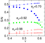
Figure 1: (color online) The ratio of the shear stress to the normal stress $S/N$ versus the packing fraction $\nu$ from the simulation data ($e_{p}=0.70$ ($\blacksquare$), $0.92$ ($\bullet$), and $0.98$ ($\circ$)) and the plot of Eq. (20) from the kinetic theory ($e_{p}=0.70$ ($*$ connected by dashed line), $0.92$ ($+$ connected by dashed line), and $0.98$ ($\times$ connected by dashed line). For the simulation data, the average normal stress $N=\frac{1}{3}(N_{x}+N_{y}+N_{z})$ is used.

In this paper, we study the velocity correlation in the sheared granular flow, focusing its effects on the energy dissipation rate and the stress. We adopt the simple shear flow of the inelastic hard spheres as a model system, in accordance with most of the kinetic theory analysis. Note that the enduring contacts is not allowed in the hard sphere model, whose effects are often under debate in the soft-sphere model simulations of the slope flow Silbert ; Mitarai .

This paper is organized as follows. In section II, we briefly summarize the inelastic hard sphere model and the constitutive relations based on the kinetic theory. We summarize our simulation method and present the results in section III. The discussion and the summary are given in section IV.

II Inelastic hard sphere model and the kinetic theory

The inelastic hard sphere model is one of the simplest and widely-used models of granular materials rapid ; Duran . The particles are infinitely rigid, and they interact through instantaneous two-body collisions. We adopt the simplest collision rule for the monodisperse smooth hard spheres with diameter $\sigma$, mass $m$, and a constant normal restitution coefficient $e_{p}$ in three dimensions as follows: The particle $i$ at the position $\bm{r}_{i}$ with the velocity $\bm{c}_{i}$ collides with the particle $j$ if $|\bm{r}_{i}-\bm{r}_{j}|=\sigma$ and $(\bm{r}_{i}-\bm{r}_{j})\cdot(\bm{c}_{i}-\bm{c}_{j})<0$, and their post-collisional velocities $\bm{c}_{i}^{*}$ and $\bm{c}_{j}^{*}$ are given by

$$\bm{c}_{i}^{*} = \bm{c}_{i}-\frac{1+e_{p}}{2}\left[\bm{n}_{ij}\cdot\left(\bm{c}_{i}-\bm{c}_{j}\right)\right]\bm{n}_{ij},$$ (4)

$$\bm{c}_{j}^{*} = \bm{c}_{j}+\frac{1+e_{p}}{2}\left[\bm{n}_{ij}\cdot\left(\bm{c}_{i}-\bm{c}_{j}\right)\right]\bm{n}_{ij},$$ (5)

respectively. Here, $\bm{n}_{ij}$ is a unit vector defined as $\bm{n}_{ij}=(\bm{r}_{i}-\bm{r}_{j})/|\bm{r}_{i}-\bm{r}_{j}|$. The collision is elastic when $e_{p}=1$, and inelastic when $0<e_{p}<1$. In the inelastic case, the particles lose the kinetic energy every time they collide, thus external drive is necessary to keep particles flowing.

We compare the simulation results of the inelastic hard spheres with the constitutive relations obtained from the Chapman-Enskog method Chapman , which has been developed in the kinetic theory of gases. In this paper, we employ those by Garzó and Dufty Garzo , who have improved the previous studies rapid ; Jenkins ; Lun , that is limited to the weakly inelastic case ($(1-e_{p})\ll 1$), to include the case with any value of the restitution constant $e_{p}$ under the assumption that the state is near the local homogeneous cooling state comment2 .

In the following, we briefly summarize the kinetic theory to derive the constitutive relations. The hydrodynamic variables are the number density field $n(\bm{r},t)$, the velocity field $\bm{u}(\bm{r},t)$, and the granular temperature field $T(\bm{r},t)$, defined in terms of the single-particle distribution function $f(\bm{r},\bm{c},t)$ as

$$n(\bm{r},t) = \int f(\bm{r},\bm{c},t)\mbox{d}\bm{c},$$ (6)

$$\bm{u}(\bm{r},t) = \frac{1}{n}\int\bm{c}f(\bm{r},\bm{c},t)\mbox{d}\bm{c},$$ (7)

$$T(\bm{r},t) = \frac{m}{3n}\int(\bm{c}-\bm{u})^{2}f(\bm{r},\bm{c},t)\mbox{d}\bm{c}.$$ (8)

The hydrodynamic equations for these variables are given by

$$\frac{\partial n}{\partial t}+\nabla\cdot(n\bm{u}) = 0,$$ (9)

$$mn\frac{\partial\bm{u}}{\partial t}+mn\bm{u}\cdot\nabla\bm{u} = -\nabla\tensor{\Sigma},$$ (10)

$$\frac{3}{2}\left(n\frac{\partial T}{\partial t}+n\bm{u}\cdot\nabla T\right) = -\nabla\cdot\bm{q}-\tensor{\Sigma}:\tensor{E}-\Gamma,$$ (11)

where $\tensor{\Sigma}$ is the stress tensor, $\bm{q}$ is the heat flux, and $\tensor{E}$ is the symmetrized velocity gradient tensor: $E_{ij}=\frac{1}{2}(\frac{\partial}{\partial r_{i}}u_{j}+\frac{\partial}{\partial r_{j}}u_{i})$. Note that the energy dissipation rate $\Gamma$ in Eq. (11) appears due to the energy loss through the inelastic collisions, which gives peculiar features to the granular hydrodynamics.

The constitutive relations for $\tensor{\Sigma}$, $\bm{q}$, and $\Gamma$ are determined by the single-particle distribution $f(\bm{r},\bm{c},t)$. Its time evolution depends on the two-particle distribution function $f^{(2)}(\bm{r}_{1},\bm{r}_{2},\bm{c}_{1},\bm{c}_{2},t)$ through the two-particle collision; the $n$-particle distribution function depends on the ($n+1$)-particle distribution function. This is known as the BBGKY hierarchy SimpleLiquid .

In the Enskog approximation, the two-particle distribution at collision is approximated as

$$f^{(2)}(\bm{r}_{1},\bm{r}_{1}+\sigma\bm{n}_{21},\bm{c}_{1},\bm{c}_{2},t)$$ (12)

$$= g_{0}(\nu)f(\bm{r}_{1},\bm{c}_{1},t)f(\bm{r}_{1}+\sigma\bm{n}_{21},\bm{c}_{2},t)$$

to close the BBGKY hierarchy at the single-particle distribution Chapman ; Garzo . Here, $g_{0}(\nu)$ is the radial distribution function at distance $\sigma$, and depends on the packing fraction $\nu=\frac{1}{6}\pi\sigma^{3}n$. The term $g_{0}(\nu)$ represents the positional correlations, and the actual procedure to determine the functional form of $g_{0}(\nu)$ is presented in subsection III.2.1. The correlations in the particle velocities are neglected under the molecular chaos assumption.

Table 1: The dimensionless functions in the constitutive relations from Ref. Garzo .

$f_{1}(\nu)$	$\frac{6}{\pi}\nu(1+2(1+e_{p})\nu g_{0}(\nu))$
$f_{2}(\nu)$	$\frac{5}{16\sqrt{\pi}}\left[\eta^{k*}\left(1+\frac{4}{5}\nu g_{0}(\nu)(1+e_{p})\right)+\frac{3}{5}\gamma^{*}\right]$
$f_{3}(\nu)$	$\frac{72(1-e_{p}^{2})}{\pi^{3/2}}\nu^{2}g_{0}(\nu)\left(1+\frac{3}{32}c^{*}(e_{p})\right)$
$\eta^{k*}$	$\left(\nu_{\eta}^{*}-\frac{1}{2}\zeta^{(0)*}\right)^{-1}\left(1-\frac{2}{5}(1+e_{p})(1-3e_{p})\nu g_{0}(\nu)\right)$
$\nu_{\eta}^{*}$	$g_{0}(\nu)(1-\frac{1}{4}(1-e_{p})^{2})(1-\frac{1}{64}c^{*}(e_{p}))$
$\zeta^{(0)*}$	$g_{0}(\nu)\frac{5}{12}(1-e_{p}^{2})(1+\frac{3}{32}c^{*}(e_{p}))$
$\gamma^{*}$	$\frac{128}{5\pi}\nu^{2}g_{0}(\nu)(1+e_{p})(1-\frac{1}{32}c^{*}(e_{p}))$
$c^{*}(e_{p})$	$32(1-e_{p})(1-2e_{p}^{2})[81-17e_{p}+30e_{p}^{2}(1-e_{p})]^{-1}.$

The constitutive relations for the hydrodynamic equations have been obtained in ref. Garzo by the Chapman-Esnkog method with the approximation (12) up to the Navier-Stokes order (i.e. the first order of the spatial gradients). In the simple steady shear flow with constant $n$, constant $T$, and $\bm{u}(\bm{r})=(\dot{\gamma}z,0,0)$, the nonzero terms are the pressure, or the normal stress

$$N_{\alpha}\equiv\Sigma_{\alpha,\alpha}=N(\nu,T)=\sigma^{-3}f_{1}(\nu)T,$$ (13)

the shear stress

$$S\equiv\Sigma_{x,z}=\Sigma_{z,x}=S(\nu,T)=m^{1/2}\sigma^{-2}f_{2}(\nu)\sqrt{T}\dot{\gamma},$$ (14)

and the energy dissipation rate

$$\Gamma=\Gamma(\nu,T)=m^{-1/2}{\sigma^{-4}}f_{3}(\nu)T^{3/2}.$$ (15)

The dimensionless functions $f_{i}(\nu)$ are listed in Table 1.

In the simple shear flow, Eqs. (9) and (10) are automatically satisfied with the constant normal stress $N$ and the constant shear stress $S$. The energy balance equation (11) gives

$$S\dot{\gamma}-\Gamma=0,$$ (16)

because there is no heat flux ${\bm{q}}$. Equation (16) means that the granular temperature is locally determined by the balance between the viscous heating and the energy dissipation. Equation (16) with Eqs. (14) and (15) gives

$$T=m\sigma^{2}\frac{f_{2}(\nu)}{f_{3}(\nu)}\dot{\gamma}^{2}.$$ (17)

Substituting Eq. (17) into Eqs. (13) and (14), we get

$$N = m\sigma^{-1}\frac{f_{1}(\nu)f_{2}(\nu)}{f_{3}(\nu)}\dot{\gamma}^{2},$$ (18)

$$S = m\sigma^{-1}\frac{[f_{2}(\nu)]^{3/2}}{[f_{3}(\nu)]^{1/2}}\dot{\gamma}^{2},$$ (19)

which are exactly what we have anticipated from the Bagnold scaling Eqs. (1) and (2).

The above derivation of the Bagnold scaling by the kinetic theory gives the definite expression for Eq. (3),

$$\frac{S}{N}=\frac{\sqrt{f_{2}(\nu)f_{3}(\nu)}}{f_{1}(\nu)},$$ (20)

as a function of the packing fraction $\nu$. This is plotted in Fig. 1 by symbols connected by lines, along with the simulation data. One can see clear discrepancy between the theory and the simulation especially in the higher density region. The kinetic theory gives increasing functions $S/N$ of $\nu$, which means that the flow down steeper slope is denser.

III Simulations

In this section, we compare the expressions Eqs. (13)-(15) with the simulation results of simple shear flow of inelastic hard spheres.

III.1 Simulation setup

The simulation is done under the constant volume condition with a uniform shear in a rectangular box of the size $L_{x}\times L_{y}\times L_{z}$. The shear is applied by the Lees-Edwards shearing periodic boundary conditions in the $z$ direction Lees-Edwards ; The periodic boundary condition is employed in the $x$ and $y$ directions. We employ the event driven method, using the fast algorithm developed by Isobe isobe .

A steady shear flow with the mean velocity $\bm{u}(\bm{r})=(\dot{\gamma}z,0,0)$ is prepared as follows. First, a random configuration is prepared by the compressing procedure proposed by Lubachevsky and Stillinger Lubachevski90 in the elastic system without shear under the periodic boundary condition. Secondly, the initial shear flow is constructed from the above random configuration by giving the initial mean velocity $\bm{u}(\bm{r})=(\dot{\gamma}z,0,0)$ and setting the initial temperature $T\approx 100m\sigma^{2}\dot{\gamma}^{2}$. Lastly, the steady shear flow of the inelastic system is obtained by relaxing the initial flow under the Lees-Edwards shearing periodic boundary condition comment3 .

With the present parameter and system size, the final steady state is the simple shear flow with uniform packing fraction $\nu=\nu_{0}$ and mean velocity $\bm{u}=(\dot{\gamma}z,0,0)$ commentS . All the following data are taken in the steady state, and averaged over the space and time (typically over 10,000 collisions per particle) unless otherwise noted.

In the following, all the quantities are given in the dimensionless form with the unit mass $m$, the unit length $\sigma$, and the unit time $\dot{\gamma}^{-1}$. Most of the data are from the simulations with system size $L_{x}=20$, $L_{y}=10$, and $L_{z}=40$. Several simulations has been done with $L_{x}=L_{y}=L_{z}=40$ to check the system size effect. We measure the temperature $T$, the normal stress $N$, the shear stress $S$, and the energy dissipation rate $\Gamma$ for various values of the packing fraction $\nu$. These are compared with Eqs.(13)-(15) from the kinetic theory.

III.2 Simulation results

III.2.1 The radial distribution function

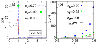
Figure 2: (color online)(a)The radial distribution functions for $\nu=0.58$ with $e_{p}=0.7$ (dashed line), $0.92$ (dotted line), and $0.98$ (solid line). The peak values of contact are 136 (out of range), 30.6 ($\bullet$), and 17.4 ($\circ$) for $e_{p}$=0.70, 0.92, and 0.98, respectively. The theoretical value at contact, $g_{0,{\rm T}}(0.58)$, is shown by an arrow. (b) Plot of $g_{0,{\rm m}}(\nu)$ versus the packing fraction $\nu$ for $e_{p}=0.7$ ($\blacksquare$), $0.92$ ($\bullet$), and $0.98$ ($\circ$). $g_{0,{\rm T}}(\nu)$ is shown by a solid line.

For the constitutive relations with Table 1, we need to know the radial distribution function at the particle diameter, $g_{0}(\nu)$, as a function of the packing fraction. For elastic hard spheres ($e_{p}=1$) in equilibrium, the well known expression of $g_{0}(\nu)$ is the Carnahan-Starling formula SimpleLiquid

$$g_{0,{\rm CS}}(\nu)=\frac{1-\nu/2}{(1-\nu)^{3}}$$ (21)

for $0<\nu<\nu_{f}$, where $\nu_{f}$ is the freezing packing fraction and $\nu_{f}\approx 0.49$ Torquato . Torquato Torquato proposed the formula that include the higher packing fraction up to the random closed packing fraction $\nu_{c}\approx 0.64$ as

$$g_{0,{\rm T}}(\nu)=\begin{cases}g_{0,{\rm CS}}(\nu)&\mbox{for}\quad 0<\nu<\nu_{f},\\ g_{0,{\rm CS}}(\nu_{f})(\nu_{f}-\nu_{c})/(\nu-\nu_{c})&\mbox{for}\quad\nu_{f}<\nu<\nu_{c}.\end{cases}$$ (22)

As for the inelastic hard spheres under shear, a generally accepted form of $g_{0}(\nu)$ does not exist, but it has been found in several simulations that $g_{0}(\nu)$ is larger for stronger inelasticity Bizon ; Alam . Figure 2(a) shows the radial distribution $g(r)$ averaged over the all directions obtained from our shear flow simulation with the packing fraction $\nu=0.58$ for various values of $e_{p}$. The spatial mesh to measure $g(r)$ was taken as $0.001$, and the peak values of $g(r)$ around $r=1$ (at the distance of the particle diameter) are marked by symbols for $e_{p}=0.98$ and $0.92$. We can see that the peak value strongly increases for smaller $e_{p}$, and can be much larger than the value from Eq. (22) ($g_{0,{\rm T}}(0.58)$ shown by an arrow). It is quite difficult to evaluate the precise value of $g_{0}(\nu)$ from this direct measurement of $g(r)$ because of the strong increase of $g(r)$ in the limit of $r\to+1$.

The way we determine $g_{0}(\nu)$ from the simulation is through the expression of the collision frequency $\omega_{0}$ Lois ; Luding from the kinetic theory Garzo ; comment4 ,

$$\omega_{0}(\nu,T)=24g_{0}(\nu)\sqrt{T}\nu\pi^{-1/2}\left(1-\frac{1}{32}c^{*}(e_{p})\right),$$ (23)

where $c^{*}(e_{p})$ is given in Table 1. By measuring $\omega_{0}$ and $T$ for each $\nu$ from the simulation, we can evaluate

$$g_{0,{\rm m}}(\nu;T,\omega_{0})\equiv\frac{\omega_{0}\sqrt{\pi}}{24(1-c^{*}(e_{p})/32)\sqrt{T}\nu}.$$ (24)

$g_{0,{\rm m}}(\nu;T,\omega_{0})$ is plotted versus $\nu$ for various values of $e_{p}$ in Fig. 2(b), where $g_{0,{\rm T}}(\nu)$ in Eq. (22) is shown by a solid line for reference. $g_{0,{\rm m}}(\nu;T,\omega_{0})$ shows stronger increase upon increasing the packing fraction $\nu$ as $e_{p}$ gets smaller; by comparing it with Fig. 2(a), we see that this indirect estimate gives an reasonable $e_{p}$ dependence of $g_{0}(\nu)$. In the following, we use $g_{0,{\rm m}}(\nu;T,\omega_{0})$ as $g_{0}(\nu)$ in Table 1 unless otherwise noted.

III.2.2 The energy dissipation rate and the normal stress as functions of the packing fraction

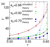
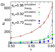
Figure 3: (color online) The energy dissipation rate $\Gamma$ (a) and the normal stress $N$ (b). The simulation data for $e_{p}=0.98$ ($\circ$), $0.92$ ($\bullet$), and $0.70$ ($\blacksquare$) are compared with the values from the kinetic theory ($\Gamma(\nu,T)$ and $N(\nu,T)$) shown by symbols connected by dashed lines for $e_{p}=0.98$ ($\times$), $0.92$ (+), and $0.70$ ($*$). $\Gamma(\nu,T_{\rm coll})$ and $N(\nu,T_{\rm coll})$ with $g_{0,{\rm m}}(\nu;T_{\rm coll},\omega_{0})$ are denoted by the solid lines, which agree with the simulation data (see text).

In Fig. 3, the energy dissipation rate $\Gamma$ (a) and the normal stress $N$ (b) are shown for various values of the packing fraction $\nu$ and the restitution coefficient $e_{p}$. For the normal stress, we find in the simulation that $N_{\alpha}$ depends on the direction $\alpha$, but the differences among them are at most $10\%$ in the plotted region and are not significant compared to the difference from the kinetic theory that we will study in the following. Thus, here we plot the average $N\equiv(N_{x}+N_{y}+N_{z})/3$.

The value from the kinetic theory are shown in Fig. 3(a) and (b) by symbols connected by dashed lines. We see in Fig. 3(a) that the energy dissipation rate is overestimated by the theory in the dense region, and the disagreement is larger for smaller $e_{p}$. The normal stress in Fig. 3(b) also shows a similar tendency, although the relative disagreements are smaller than those in the energy dissipation rate $\Gamma$.

III.2.3 The pre-collisional velocity correlation effects and the collisional temperature

The energy dissipation.

We first focus on the discrepancy in the energy dissipation rate $\Gamma$. From the collision rule Eq. (5), the energy dissipated per collision is given by

$$\Delta E_{ij}=(1-e_{p}^{2})\frac{1}{4}c_{n,ij}^{2},$$ (25)

where $c_{n,ij}\equiv\left[\left(\bm{c}_{i}-\bm{c}_{j}\right)\cdot\bm{n}_{ij}\right]$ is the relative normal velocity of colliding particles just before the collision. Thus, $\Gamma$ is given by

$$\Gamma=<\Delta E_{ij}>_{\rm coll}\cdot\frac{1}{2}n\omega_{0}=(1-e_{p}^{2})\cdot\frac{1}{4}<c_{n,ij}^{2}>_{\rm coll}\cdot\frac{1}{2}n\omega_{0}.$$ (26)

Here, $<A>_{\rm coll}$ denotes the average of a quantity $A$ over all collisions; if the value of $A$ is $A_{k}$ at the $k$-th collision, $<A>_{\rm coll}\equiv\sum_{k=1}^{N_{\rm coll}}A_{k}/N_{\rm coll}$, where $N_{\rm coll}$ is the total number of collisions. Note that Eq. (26) is the exact expression for $\Gamma$.

On the other hand, the expression (15) from the kinetic theory with Eq. (24) gives

$$\Gamma(\nu,T)=(1-e_{p}^{2})\cdot T\left[\frac{1+3c^{*}(e_{p})/32}{1-c^{*}(e_{p})/32}\right]\cdot\frac{1}{2}n\omega_{0}(\nu,T).$$ (27)

To interpret this expression, let us consider the random collision of particles whose velocity fluctuation is given by the Maxwellian. In this case, $\frac{1}{4}<c_{n,ij}^{2}>_{\rm coll}=T$, then Eq. (26) gives

$$\Gamma=(1-e_{p}^{2})T\frac{1}{2}n\omega_{0}.$$ (28)

The difference between this and Eq. (27) comes from the deviation of the velocity distribution from the Maxwellian, but the difference is found to be small in the parameter region studied in the present paper. Therefore, from the comparison of the exact expression (26) with the kinetic theory expression Eq. (27), we conclude that the deviation found in Fig. 3(a) comes from the fact that $\frac{1}{4}<c_{n,ij}^{2}>_{\rm coll}\ll T$.

The collisional temperature.

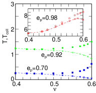
Figure 4: (color online) The temperature $T$ and “the collisional temperature” $T_{\rm coll}$ vs. the packing fraction $\nu$. $T$ and $T_{\rm coll}$ are denoted by $\blacksquare$ and $*$ with the dashed lines for $e_{p}=0.7$, respectively, and by $\bullet$ and $+$ with the dashed lines for $e_{p}=0.92$. The inset shows $T$ and $T_{\rm coll}$ for $e_{p}=0.98$ represented by $\circ$ and $\times$ with the dashed lines.

To confirm this idea, we define “the collisional temperature” $T_{\rm coll}\equiv<c_{n,ij}^{2}>_{\rm coll}/4$. Figure 4 shows $T_{\rm coll}$ and $T$ as functions of $\nu$. One can see that $T_{\rm coll}$ is substantially smaller than $T$ for $\nu>0.5$ as is concluded above.

To demonstrate that the discrepancy is actually resolved by $T_{\rm coll}$, we plot $\Gamma(\nu,T)$ of Eq. (15) with $g_{0,{\rm m}}(\nu,T,\omega_{0})$ of (24) in $f_{3}(\nu)$ replacing $T$ by $T_{\rm coll}$ (the solid lines in Fig.3(a)); This is equivalent to replace $T$ in Eq. (27) with $T_{\rm coll}$ and use the measured value of the collision frequency for $\omega_{0}$. The agreement is quite good.

Normal stress.

Now, we consider the effect of $T_{\rm coll}<T$ on the normal stress $N$. The value of $c_{n,ij}$ should also play an important role in the collisional component of the normal stress $N_{\rm coll}$, because $c_{n,ij}$ directly determines the momentum transfer from the particle $i$ to the particle $j$ through a collision: $\Delta\bm{p}_{j}\equiv(\bm{c}_{j}^{*}-\bm{c}_{j})=[(1+e_{p})/2]\ c_{n,ij}\bm{n}_{ij}=-\Delta\bm{p}_{i}$. Thus, we expect that $N_{\rm coll}$ is approximately proportional to $<|\Delta\bm{p}|>n\omega_{0}\propto\sqrt{T_{\rm coll}}n\omega_{0}$. In addition, the collisional part $N_{\rm coll}$ is dominant in the dense region.

In Fig. 3(b), $N(\nu,T_{\rm coll})$ of Eq. (13) is plotted by the solid lines, where $g_{0,{\rm m}}(\nu;T_{\rm coll},\omega_{0})$ is used as $g_{0}(\nu)$. We see that the solid lines show reasonably good agreement with the data for the whole density region.

III.2.4 Origin of the pre-collisional velocity correlation

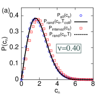
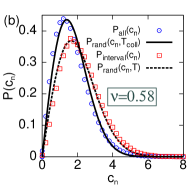
Figure 5: (color online) The distribution of relative normal velocity just before the collision $c_{n}$. $P_{\rm all}(c_{n})$ and $P_{\rm interval}(c_{n})$ are compared along with $P_{\rm rand}(c_{n};T_{\rm coll})$ and $P_{\rm rand}(c_{n};T)$ for $e_{p}=0.92$ with $\nu=0.40$ (a) and $\nu=0.58$ (b). We see that the difference between $P_{\rm all}(c_{n})$ ($\circ$) and $P_{\rm interval}(c_{n})$ ($\square$) is small for $\nu=0.40$, but for $\nu=0.58$, the $P_{\rm all}(c_{n})$ has sharper distribution. The solid lines show $P_{\rm rand}(c_{n};T_{\rm coll})$ and the dashed lines show $P_{\rm rand}(c_{n};T)$. See text for details.

Figure 6: (color online) The pre-collisional relative normal velocity distributions $P_{\rm all}(c_{n})$ ($\circ$) and $P_{\rm interval}(c_{n})$ ($\square$) compared along with $P_{\rm rand}(c_{n};T_{\rm coll})$ (solid line) and $P_{\rm rand}(c_{n};T)$ (dashed line), respectively, for $e_{p}=0.70$ with $\nu=0.58$.

One of the possible origins of the pre-collisional velocity correlation that makes $T_{\rm coll}<T$ is the inelasticity, which makes the relative normal velocity smaller upon collision. In this subsection, we examine how the pre-collisional velocity correlation develops in the shear flow.

It is expected that the correlation grows when particles collide with same colliding partners inelastically many times within a short period of time. Under the shear, however, this correlation will be lost when they are forced to pass each other and collide with new partners. The typical time scale that a pair of particles pass each other is the unit time, i.e., $\dot{\gamma}^{-1}$. This argument explains the smaller $T_{\rm coll}$ in the denser region, because particles collide more frequently with same partners before they move far apart comment5 .

This argument tells that the collision does not have memories of the previous collisions earlier than the unit time $\dot{\gamma}^{-1}$. To confirm this, we compare the following two distributions of the pre-collisional velocity: (i)$P_{\rm all}(c_{n})$, which is the distribution of $c_{n,ij}$ for all collisions between all pairs of particles, and (ii) $P_{\rm interval}(c_{n})$, which is the distribution of $c_{n,ij}$ of the collisions whose colliding pairs of particles did not collide with each other during the last unit time $\dot{\gamma}^{-1}$. If the velocity correlation mainly comes from the multiple collision with same partners within the unit time scale, then $P_{\rm interval}(c_{n})$ should have the width determined not by $T_{\rm coll}$ but by the average temperature $T$.

The results are shown in Fig. 5 for $e_{p}=0.92$ with $\nu=0.40$ (a) and $0.58$ (b), where $P_{\rm all}(c_{n})$ is denoted by $\circ$ and $P_{\rm interval}(c_{n})$ is denoted by $\square$. We see that $P_{\rm interval}(c_{n})$ is wider than $P_{\rm all}(c_{n})$ for the denser case (b).

If the particles with the Maxwellian velocity distribution with temperature $\tilde{T}$ collide among themselves randomly, the distribution of $c_{n}$ is given by

$$P_{\rm rand}(c_{n};\tilde{T})=\frac{c_{n}}{2\tilde{T}}\exp\left[-\frac{c_{n}^{2}}{4\tilde{T}}\right].$$ (29)

In Fig. 5, $P_{\rm rand}(c_{n};T)$ and $P_{\rm rand}(c_{n};T_{\rm coll})$ are shown by the dashed and solid lines, respectively. They are indistinguishable for $\nu=0.40$ in Fig. 5(a), but show clear difference for $\nu=0.58$ in Fig. 5(b). We find that $P_{\rm rand}(c_{n};T)$ fits $P_{\rm interval}(c_{n})$, and $P_{\rm rand}(c_{n};T_{\rm coll})$ fits $P_{\rm all}(c_{n})$, which further confirms that colliding partners are correlated in the way characterized by $T_{\rm coll}$.

For smaller $e_{p}$, the shape of the distributions deviates from Eq. (29) based on the random collision. Figure 6 shows $P_{\rm all}(c_{n})$ and $P_{\rm interval}(c_{n})$ compared along with $P_{\rm rand}(c_{n};T_{\rm coll})$ and $P_{\rm rand}(c_{n};T)$, respectively, for $e_{p}=0.70$ with $\nu=0.58$. $P_{\rm all}(c_{n})$ has sharper distribution than $P_{\rm interval}(c_{n})$, but neither of them fit well with $P_{\rm rand}(c_{n};T_{\rm coll})$ nor $P_{\rm rand}(c_{n};T)$. This suggests stronger correlation than the case of $e_{p}=0.92$.

III.2.5 The spatial correlation in the velocity fluctuation

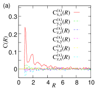
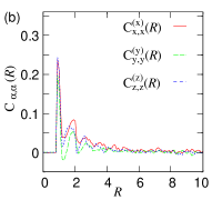
Figure 7: (color online) The spatial velocity correlation functions for $e_{p}=0.92$ and $\nu=0.55$. (a) The correlations in the $x$ direction $C^{(x)}_{\alpha,\beta}(R)$. One sees that the longitudinal component $C^{(x)}_{x,x}(R)$ (solid line) has the larger amplitude than others (shown by dashed lines). (b) The longitudinal velocity correlations $C^{\alpha}_{\alpha,\alpha}(R)$ for $\alpha=x$ (solid line), $y$ (dashed line), and $z$ (dotted line).

To understand the the velocity correlations in more detail, we study the spatial velocity correlation function defined as

$$C^{(\gamma)}_{\alpha,\beta}(R)=\frac{<\sum_{i,j}\left[\tilde{c}_{\alpha,i}\tilde{c}_{\beta,j}\Delta(R-|(\bm{r}_{i}-\bm{r}_{j})\cdot\bm{e}_{\gamma}|)\right]>}{<\sum_{i,j}\left[\Delta(R-|(\bm{r}_{i}-\bm{r}_{j})\cdot\bm{e}_{\gamma}|)\right]>},$$ (30)

where $\alpha$, $\beta$, and $\gamma$ take $x,y$ or $z$, $\tilde{c}_{\alpha,i}\equiv(c_{\alpha,i}-u_{\alpha})$, $<\cdots>$ denotes the time average, and $\bm{e}_{\gamma}$ represents the unit vector in the $\gamma$ direction. $\Delta(R-|\bm{r}\cdot\bm{e}_{\gamma}|)$ is one when $|R-|\bm{r}\cdot\bm{e}_{\gamma}||<0.05$ and $|\bm{r}\cdot\bm{e}_{\gamma^{\prime}}|<0.1$ for $\gamma^{\prime}\neq\gamma$, and it is zero otherwise. We calculated $C^{(\gamma)}_{\alpha,\beta}(R)$ for the system with $e_{p}=0.92$, both for the small system with $L_{x}=20,L_{y}=10,L_{z}=40$ and the large system with $L_{x}=40,L_{y}=40,L_{z}=40$. We find that the correlation extends over the whole system in the case of the small system, but it goes to zero for the large system. In the following, we present the spatial correlation measured in the large system, but we confirmed that the hydrodynamic quantities presented in the previous subsections did not show any differences.

In Fig. 7(a), the various components of the correlation in the $x$-direction $C^{(x)}_{\alpha,\beta}(R)$ are shown. We find that the longitudinal correlation in the $x$-direction, $C^{(x)}_{x,x}(R)$, has larger amplitude than other components; this tendency is also found in the $y$- and $z$-direction (data not shown). The longitudinal correlation at the particle diameter distance ($R=1$) is positive, which is consistent with the fact that $T_{\rm coll}<T$. It is evident that the correlation shows an oscillation, whose wavelength is order of the particle diameter, which will be discussed in section IV.

The longitudinal components in $x$, $y$ and $z$ directions are shown in Fig. 7(b). All of them show oscillations in the particle diameter scale. We also found that the longitudinal correlation shows larger amplitude for smaller restitution coefficient $e_{p}$ and/or larger packing fraction $\nu$ (data not shown).

III.2.6 The packing fraction dependence of the shear stress

We find that the shear stress $S$ shows more complicated packing fraction $\nu$ dependence than those of the energy dissipation rate $\Gamma$ and the normal stress $N$. In Fig.8, the simulation data of the shear stress $S$ are denoted by symbols, and $S(\nu,T)$ from the kinetic theory (Eq. (14) with Table 1) are denoted by symbols with the dashed lines. We find that, for $e_{p}=0.98$, the shear stress is underestimated by the theory, while for $e_{p}=0.92$ and $0.70$, the shear stress is overestimated.

Actually, in the case of the elastic ($e_{p}=1$) hard sphere system, the Enskog theory is known to underestimate the shear viscosity in dense region SimpleLiquid ; Alder , and this tendency is seen in the result for $e_{p}=0.98$. The results for $e_{p}=0.70$ shows that the inelasticity reduces the shear stress to the value smaller than the one expected from the kinetic theory, but we do not understand the reason of this reduction yet. Rather good agreement in between for the case of $e_{p}=0.92$ seems to be accidental.

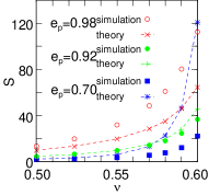
Figure 8: (color online) The shear stress $S$ vs. the packing fraction $\nu$. The simulation data are plotted for $e_{p}=0.98$ ($\circ$), $0.92$ ($\bullet$), and $0.70$ ($\blacksquare$). The kinetic theory constitutive relations $S(\nu,T)$ is shown by the symbols connected by dashed lines ($\times$ for $e_{p}=0.98$, $+$ for $0.92$, and $*$ for $e_{p}=0.70$).

IV Discussion and summary

IV.1 The shear stress and the anisotropic correlation

In contrast to the energy dissipation rate $\Gamma$ and the normal stress $N$, the discrepancy in the shear stress $S$ cannot be understood just by the pre-collisional velocity distribution averaged over all directions, but the anisotropy of the pre-collisional correlations in both the velocity and the position should by important in the shear stress. These anisotropies are not taken into account in the kinetic theory employed in the preset analysis. In fact, for the soft-sphere system in two-dimensional, sheared flow, it has been found that the contact force distribution strongly depends on direction Cruz . Our preliminary results also show a similar direction dependence in the collisional momentum transfer per unit time. The detailed analysis is left for future studies.

IV.2 The packing fraction dependence of the ratio of the shear stress to the normal stress

As we have seen in Fig. 1, $S/N$ in the simulation is a decreasing function of the packing fraction $\nu$ for larger packing fraction $\nu$ and/or smaller restitution coefficient $e_{p}$, while Eq. (20), from the kinetic theory, $S/N$ always increases with $\nu$.

Kumaran argued that the particle roughness is necessary for $S/N$ to have a decreasing part upon increasing $\nu$ in the dense region Kumaran . However, even for the smooth particles, the present simulations show that $S/N$ has a decreasing part in the dense region for the inelastic hard sphere system, although the particle roughness may well amplify the decreasing part of $S/N$.

The present authors have suggested Mitarai that the origin that leads the kinetic theory to the increasing $S/N$ on $\nu$ even for the denser region is that $f_{3}(\nu)$ in the energy dissipation $\Gamma$ of Eq. (15) increases too sharply for larger $\nu$. In this paper in section III.2.3, we showed that the sharp increase in $\Gamma$ can be weaken by using $T_{\rm coll}$ instead of $T$. In the present treatment, however, It is not possible to extract the $\nu$-dependence out of $\Gamma(\nu,T_{\rm coll})$ and to compare it directly with $f_{3}(\nu)$ because $T$ and $T_{\rm coll}$ are determined by $\nu$ and $\dot{\gamma}$ in the steady state simulations, therefore, the quantity that corresponds to $f_{3}(\nu)$ in eq. (15) cannot be defined from the simulation data.

Finally, let us comment on the fact that $S/N$ does increase with $\nu$ in a certain parameter range in our simple shear flow simulation, in contrast to the fact that the increasing $\nu$ upon increasing $S/N=\tan\theta$ has never been observed in the granular flow down a slope. This suggests that the steady flow in this parameter region is unstable in the slope flow configuration. It is interesting to study the relation between the stability of the flow and the $\nu$ dependence of $S/N$.

IV.3 Oscillation in the spatial velocity correlation

As shown in Fig. 7, the spatial velocity correlation is found to oscillate in the scale of the particle diameter. Although we have not yet understood the origin of this oscillation, it is plausible that the oscillation comes from the coupling between the density correlation and the velocity correlation. Analysis on the sheared Langevin system suggests that the spatial velocity correlation is related to the radial distribution function Yoshimori , which oscillates in the particle diameter scale. It is likely that similar coupling also exists in the granular shear flow.

IV.4 Summary

We have simulated the simple shear flow of the smooth inelastic hard sphere system by molecular dynamics simulations. We have found that the energy dissipation rate $\Gamma$ and the normal stress $N$ are smaller than those expected from the kinetic theory. We have showed that the relative pre-collisional normal velocity of colliding pairs of particles, $c_{n,ij}$, is smaller than the one expected from random collisions, and this reduces $\Gamma$ and $N$. By examining the distributions of $c_{n,ij}$ for all collisions ($P_{\rm all}(c_{n})$) and for only the first collisions of the new pairs during the last period of time $\dot{\gamma}^{-1}$ ($P_{\rm interval}(c_{n})$), we have concluded that the reduction of the relative velocity is caused by the multiple inelastic collisions during the time period $\dot{\gamma}^{-1}$.

To understand the velocity correlation in more detail, we have studied the spatial velocity correlation. It has been found that the longitudinal components of the correlations have larger amplitude with the oscillation in the scale of the particle diameter.

The shear stress $S$ has been found to be overestimated for smaller $e_{p}$, but underestimated for larger $e_{p}$ by the kinetic theory.

- (1) S. Chapman and T. G. Cowling, “The mathematical theory of non-uniform gases (3rd ed.)”, Cambridge university press, Cambridge (1970).
- (2) J.T. Jenkins and S.B. Savage, J. Fluid Mech. 130, 187 (1983): C.S. Campbell, Annu. Rev. Fluid Mech. 22, 57 (1990).
- (3) O. Pouliquen, Phys. Fluids 11, 542 (1999).
- (4) GDRMiDi, Eur. Phys. J. E 14, 341 (2004).
- (5) L.E. Silbert, D. Ertaş, G.S. Grest, T.C. Halsey, D. Levine, and S.J. Plimpton, Phys. Rev. E 64, 051302 (2001): L.E. Silbert, G.S. Grest, S.J. Plimpton, and D. Levine, Phys. Fluids 14, 2637 (2002).
- (6) N. Mitarai and H. Nakanishi, Phys. Rev. Lett. 94, 128001 (2005).
- (7) R.A. Bagnold, Proc. R. Soc. London A 225, 49 (1954).
- (8) C.S. Campbell, J. Fluid Mech. 465, 261 (2002): T. Hatano, M. Otsuki, and S. Sasa, arXiv:cond-mat/0607511.
- (9) L.E. Silbert, D. Ertaş, G.S. Grest, T.C. Halsey, and D. Levine, Phys. Rev. E 65, 051307 (2002).
- (10) M.Y. Louge, Phys. Rev. E 67, 061303 (2003); in Proceedings of International Conference on Multiphase Flow, Yokohama, 2004, paper no. K13.
- (11) V. Garzó and J. W. Dufty, Phys. Rev. E 59, 5895 (1999).
- (12) J.T. Jenkins, Phys. Fluids 18, 103307 (2006).
- (13) V. Kumaran, J. Fluid Mech. 561, 1 (2006).
- (14) J.T. Jenkins and M.W. Richman, Phys. Fluids 28, 3485 (1985).
- (15) C. Bizon, M.D. Shattuck, J.B. Swift, and H.L. Swinney, Phys. Rev. E 60, 4340 (1999).
- (16) M. Alam and S. Luding, Phys. Fluids 15, 2298 (2003).
- (17) R. Kawahara and H. Nakanishi, J. Phys. Soc. Jpn. 73, 68 (2004).
- (18) R. Soto, J. Piasecki, and M. Mareschal, Phys. Rev. E 64, 031306 (2001); R. Soto and M. Mareschal, ibid 63, 041303 (2001).
- (19) T.P.C. van Noije, M.H. Ernst, R. Brito and J.A.G. Orza, Phys. Rev. Lett. 79, 411 (1997); T.P.C. van Noije, M.H. Ernst, and R. Brito, Pysica A, 251, 266 (1998); T.P.C. van Noije and M.H. Ernst, Pys. Rev. E 61, 1765 (2000).
- (20) Experimentally, the spatial “velocity correlation” was studied by Pouliquen PouliquenCor in the granular flow down a slope. In the experiments, however, the velocity is measured from displacement between certain time intervals (limited by camera frames), and it is different from the simultaneous velocity correlations studied in the present paper.
- (21) O. Pouliquen, Phys. Rev. Lett. 93, 248001(2004).
- (22) J. Duran, Sands, Powders, and Grains: An Introduction To the Physics of Granular Materials (Springer, New York, 1999).
- (23) C.K.W. Lun, S.B. Savage, D.J. Jeffrey, and N. Chepurniy, J. Fluid Mech. 140, 223 (1984).
- (24) We also compared our simulation results with the constitutive relations by Lun et al. Lun that assumes weak inelasticity, but the results were almost the same in the studied parameter region.
- (25) J.P. Hansen and I.R. MacDonald, “Theory of simple liquids (2nd ed.)“ (Academic press, london, 1986)
- (26) D.J. Evans and G.P. Morriss, “Statistical mechanics of nonequilibrium liquids”, Chapter 6 (Academic press, London, 1990).
- (27) M. Isobe, Int. J. Mod. Phys. C 10, 1281 (1999).
- (28) D. Lubachevski and F.H. Stillinger, J. Stat. Phys. 60, 561 (1990).
- (29) In the case of the small restitution coefficient (e.g. ), the system often encounters the inelastic collapse Collapse ; CollapseShear before reaching the steady state unless we start the simulation with the initial mean flow. With the initial mean flow, the system may reach a steady shear flow, but the inelastic collapse may eventually occur even with shear CollapseShear . In this paper, we focus on the results of the simulations where the inelastic collapse did not occur within the run.
- (30) The simple uniform shear flow can be unstable for large system stability , but we do not pursue the condition for its stability.
- (31) S.B. Savage, J. Fluid Mech. 241, 109 (1992); M. Babic, ibid 254, 127 (1993); V. Kumaran, ibid 506, 1 (2004); K. Saitoh and H. Hayakawa, arXiv:cond-mat/0604160.
- (32) B. Berne and R. Mazighi, J.Phys.A:Math.Gen.23, 5745(1990); S. McNamara and W.R. Young, Phys.Fluids A 4,496 (1992); Phys. Rev.E 50, R28 (1994); 53, 5089 (1996)
- (33) M. Alam and C.M. Hrenya, Phys. Rev. E 63, 061308 (2001).
- (34) S. Torquato, Phys. Rev. E 51, 3170 (1995).
- (35) S. Luding and A. Santos, J.Chem.Phys. 121,8458 (2004).
- (36) G. Lois, A. Lemaitre, and J. M. Carlson, Europhys. Lett. 76, 318 (2006).
- (37) In ref. Garzo , the collision frequency was not explicitly calculated, but the value of the necessary integral was given.
- (38) In the denser region of the shear flow, i.e. with smaller free volume, the particles tends to move collectively and this may also create the velocity correlation in the dense regime even without inelasticity. In any case, the collective motion is broken by the shear, and the time scale that the shear breaks the correlation is about the unit time ().
- (39) A. Yoshimori, private communication.
- (40) B.J. Alder and T.E. Wainwright, Phys. Rev. A 1 18 (1970).
- (41) F. da Cruz, S. Emam, M. Prochnow, J.-N. Roux, and F. Chevoir, Phys. Rev. E 72, 021309 (2005).