Stochastic $\bf\varphi^{4}-$Theory in the Strong Coupling Limit

Abstract

The stochastic $\varphi^{4}$-theory in $d-$dimensions dynamically develops domain wall structures within which the order parameter is not continuous. We develop a statistical theory for the $\varphi^{4}$-theory driven with a random forcing which is white in time and Gaussian-correlated in space. A master equation is derived for the probability density function (PDF) of the order parameter, when the forcing correlation length is much smaller than the system size, but much larger than the typical width of the domain walls. Moreover, exact expressions for the one-point PDF and all the moments $\langle\varphi^{n}\rangle$ are given. We then investigate the intermittency issue in the strong coupling limit, and derive the tail of the PDF of the increments $\varphi(x_{2})-\varphi(x_{1})$. The scaling laws for the structure functions of the increments are obtained through numerical simulations. It is shown that the moments of field increments defined by, $C_{b}=\langle|\varphi(x_{2})-\varphi(x_{1})|^{b}\rangle$, behave as $|x_{1}-x_{2}|^{\xi_{b}}$, where $\xi_{b}=b$ for $b\leq 1$, and $\xi_{b}=1$ for $b\geq 1$.

PACS: 05.10.Gg,11.10.Lm

]

I Introduction

Thirty five years ago Wilson and Fisher [1] emphasized the relevance of the $\varphi^{4}$-theory to understanding the critical phenomena. Since then, the theory has become one of the most appealing theoretical tools for studying the critical phenomena in a wide variety of systems in statistical physics. In the strong coupling limit, the $\varphi^{4}$-theory develops domain walls, a phenomenon which is of great interest in the classical and quantum field theories [2-10]. The dynamical $\varphi^{4}-$theory - what is usually referred to as the time-dependent Ginzburg-Landau (GL) theory - provides a phenomenological approach to, and plays an important role in, understanding dynamical phase transitions and calculating the associated dynamical exponent [11-16]. The time-dependent GL theory for superconductors was presented phenomenologically only in 1968 by Schmid [17] (and derived from microscopic theory shortly thereafter [18]), when the first modulational theory was derived in the context of Rayleigh-Benard convection [19, 20]. Moreover, the GL equation with an additional noise term has been studied intensively as a model of phase transitions in equilibrium systems; see, for example, [21].

In the present paper we consider the stochastic $\varphi^{4}$-theory in the strong coupling limit. This limit is singular in the sense that, the equation that describes the dynamics of the system develops singularities. Therefore, starting with a smooth initial condition, the domain-wall singularities are dynamically developed after a finite time. At the singular points the field $\varphi(x,t)$ is not continuous. We derive master equations for the joint probability density functions (PDF) of $\varphi$ and its increments in $d$ dimensions. It is shown that in the stationary state, where the singularities are fully developed, the relaxation term in the strong coupling limit leads to an unclosed term in the PDF equations.

Using the boundary layer method [22, 23], we show that the unclosed term makes no finite contribution (anomaly) in the strong coupling limit, and derive the PDF of $\varphi$ and its moments, $\langle\varphi^{n}\rangle$, in the same limit. We also investigate the scaling behavior of the moments of the field’s increments defined by, $\delta\varphi=\varphi(x_{2})-\varphi(x_{1})$, and show that when $|x_{2}-x_{1}|$ is small, fluctuations of the $\varphi$ field have a bi-fractal structure and are intermittent. The intermittency implies that the structure function defined by, $C_{b}=\langle|\varphi(x_{2})-\varphi(x_{1})|^{b}\rangle$, scales as $|x_{2}-x_{1}|^{\zeta_{b}}$, where $\zeta_{b}$ is a nonlinear function of $b$. It is also shown numerically that the moments of the field’s increments, $\langle|\varphi(x_{2})-\varphi(x_{1})|^{b}\rangle$, behave as, $|x_{2}-x_{1}|^{\xi_{b}}$, where $x_{b}=b$ for $b\leq 1$, and $\xi_{b}=1$ for $b\geq 1$.

The rest of this paper is organized as follows. In the next section we present the model that we wish to study, and describe some of its properties by solving it numerically. In III and IV we derive master equations for the order parameter of the model, and for the field’s increments and its PDF tail. The numerical simulations for extracting the scaling exponents are described in V. The paper is summarized in VI, while the Appendices provide some technical details of the work that we present in the main part of the paper.

II The Model and the Coupling Constant

The standard GL $\varphi^{4}$-theory describes a second-order phase transition in any system with a one-component order parameter $\varphi(x)$ and the $\varphi\to-\varphi$ symmetry in a zero external field. The theory is described by the following action,

$$S=\int\left[-\frac{k}{2}(\nabla\varphi)^{2}+\frac{\tau}{2!}\varphi^{2}-\frac{g}{4!}\varphi^{4}\right]d^{d}x\;,$$ (1)

where $\tau=T-T_{c}$, with $T_{c}$ being the critical temperature, and $k$ is the diffusion coefficient. We consider the case in which $\tau>0$. For $d\geq 2$, the critical temperature $T_{c}$ is finite, while in one dimension (1D), $T_{c}=0$. The parameter $g$ characterizes the strength of the fluctuation interaction, or the coupling constant. The equation of motion is given by,

$$k\nabla^{2}\varphi+\tau\varphi-\frac{g}{6}\varphi^{3}=0.$$ (2)

The critical dynamics of the system is described by a stochastic equation of a particular form - the Langevin equation (for a comprehensive review on Langevin type equations see [24] )- given by

$$\frac{\partial\varphi}{\partial t}=k\nabla^{2}\varphi+\tau\varphi-\frac{g}{6}\varphi^{3}+\eta({\bf x},t)\;,$$ (3)

where $\eta({\bf x},t)$ is a Gaussian-distributed noise with zero average and the correlation function,

$$\langle\eta({\bf x},t)\eta({\bf x}^{\prime},t^{\prime})\rangle=D_{0}D({\bf x}-{\bf x}^{\prime})\delta(t-t^{\prime})\;,$$ (4)

with $D({\bf x}-{\bf x}^{\prime})$ being an arbitrary smooth function. Typically, the spatial correlation of the forcing term is considered to be a delta function in order to mimic short-range correlations. Here, though, the spatial correlation is defined by

$$D({\bf x}-{\bf x}^{\prime})=\frac{1}{({\pi\sigma^{2}})^{d/2}}\exp\left[-\frac{({\bf x}-{\bf x}^{\prime})^{2}}{\sigma^{2}}\right]\;,$$ (5)

where $\sigma\ll L$ endows a short-range character to the random forcing. It is useful to rescale Eq. (3) by writing, $\varphi^{\prime}=\varphi/\varphi_{0}$, $x^{\prime}=x/x_{0}$, and $t^{\prime}=t/t_{0}$. If we let $t_{0}=1/\tau$, $\varphi_{0}=(6\tau/g)^{1/2}$, and, $x_{0}=[(d_{0}g)/(6\tau^{2})]^{1/d}$, all the parameters are eliminated in Eq. (3) except for, $k^{\prime}=[6/(D_{0}g)]^{2/d}\tau^{4/d-1}k$, and one finds that

$$\frac{\partial\varphi}{\partial t}=k^{\prime}\nabla^{2}\varphi+\varphi-\varphi^{3}+\eta({\bf x},t)\;,$$ (6)

where $k^{\prime}$ is now the effective coupling constant of the theory. The weak and strong coupling limits of the theory are then defined, respectively, by, $k^{\prime}\to\infty$ and $k^{\prime}\to 0$. In the weak coupling limit one can use numerical simulations and the Feynman diagrams to calculate the critical exponents. On the other hand, to solve the problem in the strong coupling limit we need other techniques to derive the stochastic properties of the fluctuation field [16]. The nonlinearity of Eq. (6) in the strong coupling limit gives rise to the possibility of formation of singularity in a finite time. This means that there is a competition between the smoothing effect of diffusion (the Laplacian term) and the $\varphi^{3}$ term. Let us now describe the main properties of the GL theory in the limit, $k^{\prime}\to 0$.

i) The unforced GL model [$\eta({\bf x},t)=0$], with given initial conditions, develops singularities in any spatial dimension. In one spatial dimension (1D) the singularities are developed in a finite time $t_{c}$ as $k^{\prime}\to 0$. At such singular points the field $\varphi$, representing an order parameter, is not continuous. In 2D the unforced GL model develops domain walls, characterized by singular lines with finite lengths (that depend on the initial condition). Under these conditions, the field $\varphi$ is discontinuous when crossing the singular lines. In three and higher dimensions the structure of the singularities can be more complex. For example, in 3D the singularities are domain walls where the field $\varphi$ is discontinuous.

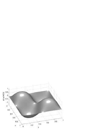
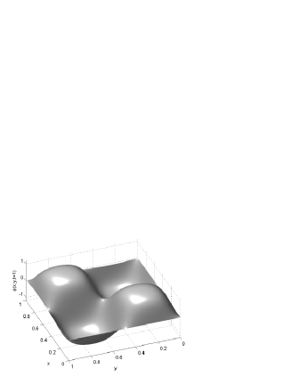
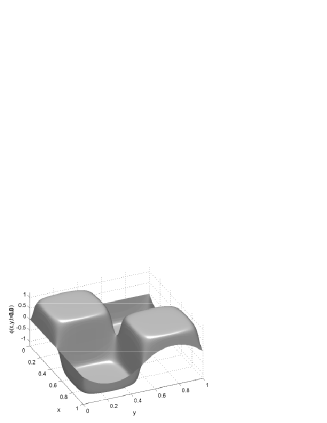
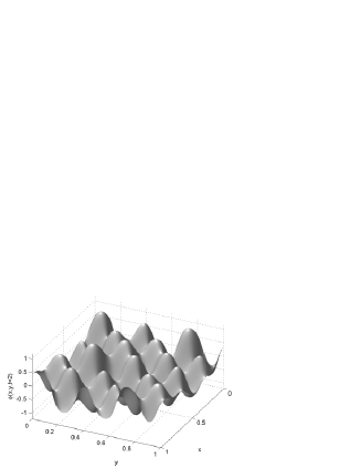
In Figs. 1 we show the time evolution of the order parameter $\varphi$ of the unforced GL model in 2D, in the limit $k^{\prime}\to 0$ [Eq. (6) with $\eta=0$]. We have used the finite-element method to numerically solve the Langevin equation with $k^{\prime}\to 0$ and the initial condition, $\varphi(x,y,0)=\sin x\sin y$. Such initial conditions are typical, and were used only for simplicity. The time scale for reaching the singularity is of the order of $k^{\prime-1/2}$. As Figs. 1a and 1b indicate, it is evident that at times $t<t_{c}$ (in the limit, $k^{\prime}\to 0$) the $\varphi$ field is continuous. At $t=t_{c}$ the $\varphi$ field becomes singular; see Fig. 1c.

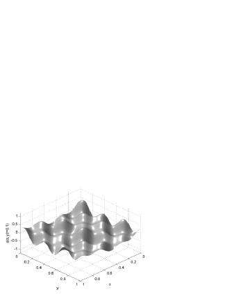
(ii) Similarly, for a forcing term which is white noise in time and smooth in space, singularities are developed in any spatial dimension in the strong coupling limit and in a finite time, $t_{\eta}=t_{c,\eta}$, as $k^{\prime}\to 0$. For example, in 2D the boundaries of the domain walls are smooth curves. In Fig. 2 we demonstrate the time evolution of the order parameter $\varphi$ of the forced GL model in 2D in the limit $k^{\prime}\to 0$. Starting from a smooth initial condition, as shown in Figs. 2a and 2b, it is evident that for times $t<t_{c,\eta}$ the $\varphi$ field is continuous. At $t=t_{c,\eta}$ the field becomes singular; see Fig. 2c.

FIG. 1.: Snapshots of the order parameter $\varphi$ at various times in the 2D unforced $\varphi^{4}$-theory in the strong coupling limit, $k^{\prime}\to 0$. Top two figures show the $\varphi$ field before the singularity develops. In the bottom figure, which is for time scales greater than the time at which singularity develops, the $\varphi(x,y)$ field is not continuous. The initial condition is, $\varphi(x,y,0)=\sin x\sin y$.

FIG. 2.: Snapshots of the order parameter $\varphi$ of a randomly-driven 2D $\varphi^{4}$-theory in the strong coupling limit. In the simulations the relation between the forcing length scale $\sigma$ and the sample size $L$ is, $\sigma\simeq L/3$. The forcing strength $D_{0}$ is 0.1.

III Master Equation of the Order Parameter

In this section we derive a master equation to describe the time evolution of the PDF $P(\varphi,t)$ of the order parameter $\varphi$. Defining a one-point generating function by, $Z(\lambda)=\langle\Theta\rangle$, where $\Theta$ is defined by, $\Theta=\exp[-i\lambda\varphi(x,t)]$. Using Eq. (6), the time evolution of $Z$ is governed by

$$Z_{t}=-i\lambda k^{\prime}\langle\nabla^{2}\varphi\exp[-i\lambda\varphi(x,t)]\rangle-i\lambda\langle\varphi\Theta\rangle$$ (7)

$$+i\lambda\langle\varphi^{3}\Theta\rangle-i\lambda\langle\eta\Theta\rangle-\lambda^{2}k(0)Z\;,$$ (8)

where, $k(x)=D_{0}D({\bf x})$, and we have invoked Novikov’s theorem (see Appendix I), which is expressed via the relation,

$$\langle\eta\exp[-i\lambda\varphi(x,t)]\rangle=-i\lambda k(0)Z\;.$$ (9)

Now, using the identities, $-i\lambda\langle\varphi\exp[-i\lambda\varphi(x,t)]\rangle=\lambda Z_{\lambda}$, and $-i\lambda\langle\varphi^{3}\exp[-i\lambda\varphi({\bf x},t)]\rangle=\lambda Z_{\lambda}\lambda\lambda$, the generating function $Z$ satisfies the following unclosed master equation

$$Z_{t}=-i\lambda k^{\prime}\langle\nabla^{2}\varphi\exp[-i\lambda\varphi(x,t)]\rangle+\lambda Z_{\lambda}+\lambda Z_{\lambda\lambda\lambda}$$ (10)

$$-\lambda^{2}k(0)Z\;.$$ (11)

The $-i\lambda k^{\prime}\langle\nabla^{2}\varphi\exp[-i\lambda\varphi(x,t)]\rangle$ term of Eq. (10) is the only one which is not closed with respect to $Z$. The PDF of order parameter $P(\varphi)$ is constructed by Fourier transforming the generating function $Z$:

$$P(\varphi,t)=\int\frac{d\lambda}{2\pi}\exp(i\lambda\varphi)Z(\lambda,t)\;.$$ (12)

Thus,

$$P_{t} = -[(\varphi-\varphi^{3})P]_{\varphi}+k(0)P_{\varphi\varphi}$$ (13)

$$- ik^{\prime}\int\frac{d\lambda}{2\pi}\lambda\exp(i\lambda\varphi)\langle\nabla^{2}\varphi\exp[-i\lambda\varphi(x,t)]\rangle\;.$$ (14)

It is evident that the governing equation for $P(\varphi,t)$ is also not closed.

Let us now use the boundary layer technique to prove that the unclosed term [the last term of Eq. (11)] makes, in the strong coupling limit, no contribution to the governing equation for the PDF[22, 23]. We consider two different time scales in the limit, $k^{\prime}\to 0$. (i) Early stages before developing the singularities ($t<t_{c,\eta}$), and (ii) in the regime of established stationary state with fully-developed sharp singularities ($t\geq t_{c,\eta}$).

In regime (i), ignoring the relaxation term in the governing equation for the PDF, one finds, in the limit $k^{\prime}\to 0$, the exact equation for the time evolution of the PDF for the order parameter (see below for more details). In contrast, the limit $k^{\prime}\to 0$ is singular in regime (ii), leading to an unclosed term (the relaxation term) in the equation for the PDF. However, we show that the unclosed term scales as $k^{\prime 1/2}$, implying that this term, in the strong coupling limit, makes no finite contribution or anomaly to the solution of Eq. (11). It is known for such time scales (the stationary state) that the $\varphi$-field, which satisfies the Langevin equation, gives rise to discontinuous solutions in the limit, $k^{\prime}\to 0$. Consequently, for finite $\sigma$ the singular solutions form a set of points where the domain walls are located, and are continuously connected. We should note that $k^{\prime}\varphi_{xx}$, in the limit $k^{\prime}\to 0$, is zero at those points at which there is no singularity. Therefore, in the limit $k^{\prime}\to 0$ only small intervals around the walls contribute to the integral in Eq. (11). Within these intervals, a boundary layer analysis may be used for obtaining accurate approximation of $\varphi({\bf x},t)$.

Generally speaking, the boundary layer analysis deals with problems in which the perturbations are operative over very narrow regions, across which the dependent variables undergo very rapid changes. The narrow regions, usually referred to as the domain walls, frequently adjoin the boundaries of the domain of interest, due to the fact that a small parameter ($k^{\prime}$ in the present problem) multiplies the highest derivative. A powerful method for treating the boundary layer problems is the method of matched asymptotic expansions. The basic idea underlying this method is that, an approximate solution to a given problem is sought, not as a single expansion in terms of a single scale, but as two or more separate expansions in terms of two or more scales, each of which is valid in some part of the domain. The scales are selected such that the expansion as a whole covers the entire domain of interest, and the domains of validity of neighboring expansions overlap. In order to handle the rapid variations in the domain walls’ layers, we define a suitable magnified or stretched scale and expand the functions in terms of it in the domain walls’ regions.

For this purpose, we split $\varphi$ into a sum of inner solution near the domain walls and an outer solution away from the singularity lines, and use systematic matched asymptotics to construct a uniform approximation of $\varphi$. For the outer solution, we look for an approximation in the form of a series in $k^{\prime}$,

$$\varphi=\varphi^{\rm out}=\varphi_{0}+k^{\prime}\varphi_{1}+O(k^{\prime 2})\;,$$ (15)

where $\varphi_{0}$ satisfies the following equation

$$\varphi_{0t}=\varphi_{0}-\varphi_{0}^{3}+\eta({\bf x},t)\;.$$ (16)

Indeed, $\varphi_{0}$ satisfies Eq. (6) with $k^{\prime}=0$. Far from the singular points or lines, the PDF of $\varphi_{0}$ satisfies the Fokker-Planck equation, with the drift and diffusion coefficients being, $D^{(1)}(\varphi_{0},t)=\varphi_{0}-\varphi_{0}^{3}$, and $D^{(2)}=k(0)$, respectively. Reference [16] gives the solution of the time-dependent Fokker-Planck equation with such drift and diffusion coefficients. At long times and in the area far from the singular points or lines, the PDF of $\varphi_{0}$ will have two maxima at $\pm 1$. This means that we are dealing with the smooth areas in Fig. 2c in the stationary state.

In order to deal with the inner solution around the domain walls, we consider the $x$ component normal to the domain wall or singularity line, and decompose the operator $\nabla^{2}$ as $\partial_{xx}+\nabla_{d-1}^{2}$. In the strong coupling limit, $k^{\prime}\to 0$, the term $\nabla_{d-1}^{2}\varphi$ makes no contribution to the PDF equation, whereas the term $\partial_{xx}\varphi$ is singular. To derive the long-time solution of Eq. (6), we rescale $x$ to $z\equiv\frac{x}{\sqrt{2k^{\prime}}}$ and suppose that complete solution of Eq. (6) has the form, $\varphi(z,t)=f(z,t)+\tanh(z)$. All the effects of the initial condition and time-dependence of $\varphi(x,t)$ will then be contained in $f(z,t)$. We now rewrite Eq. (6) with the new variables to obtain

$$\partial_{t}f(z,t)= \frac{1}{2}\partial_{zz}f(z,t)+f(z,t)-f^{3}(z,t)$$ (19)

$$-3f(z,t)\tanh(z)[f(z,t)+\tanh(z)]$$

$$+\sqrt[4]{2k^{\prime}}\eta(z,t)\;.$$

The last term of Eq. (14) is zero in the limit $k^{\prime}\to 0$. Multiplying Eq. (14) by $f(z,t)$ and integrating over $z$, one finds that,

$$\partial_{t}\int dzf^{2}(z,t)=-\int dz(\partial_{z}f(z,t))^{2}+2\int dzf^{2}(z,t)$$ (20)

$$-2\int dzf^{4}(z,t)-6\int dzf^{3}(z,t)a(z)$$ (21)

$$-6\int dza^{2}(z)f(z,t)^{2}\;,$$ (22)

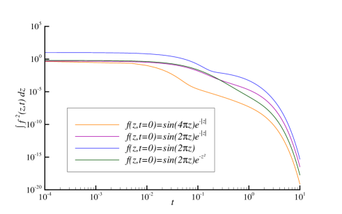
where $a(z)=\tanh(z)$. We show in Fig. (3) the time variations of $\int dzf^{2}(z,t)$ verses $t$ with different types of initial conditions. The results show that $\int dzf^{2}(z,t)$ vanishes at long times. Therefore, $\varphi(z,t)\to\tanh(z)$, in the limit of a stationary state. Let us now compute the contribution of the unclosed term in Eq. (11) in the stationary state, i.e.,

$$-k^{\prime}\int\frac{d\lambda}{2\pi}i\lambda e^{i\lambda\varphi}\langle\nabla^{2}\varphi e^{-i\lambda\varphi(x,t)}\rangle$$ (23)

(24)

$$=-k^{\prime}\left(\int\frac{d\lambda}{2\pi}e^{i\lambda\varphi}\langle\nabla^{2}\varphi e^{-i\lambda\varphi(x,t)}\rangle\right)_{\varphi}$$ (25)

$$=-k^{\prime}\langle\nabla^{2}\varphi\delta[\varphi-\varphi(x,t)]\rangle_{\varphi}$$ (26)

In the second line of Eq. (16), we have replaced $i\lambda$ with differentiation with respect to $\varphi$ and in the third line the integration of $\lambda$ has been carried through. Now, assuming ergodicity, the term $k^{\prime}\langle\nabla^{2}\varphi\delta(\varphi-\varphi(x,t))\rangle$ is converted to,

$$=-k^{\prime}\lim_{V\to\infty}\frac{1}{V}\int_{V}dxdv_{d-1}\nabla^{2}\varphi\delta[\varphi-\varphi(x,t)]\;.$$ (27)

In the limit $k^{\prime}\to 0$, only at points where we have singularity the above term is not zero. Therefore, we approach the domain walls’ regions as

$$=-k^{\prime}\lim_{V\to\infty}\frac{1}{V}\sum_{j}\int_{\Omega_{j}}dxdv_{d-1}(\varphi_{xx}+\nabla^{2}_{d-1}\varphi)$$ (28)

$$\times\delta[\varphi-\varphi(x,t)]\;,$$ (29)

where $\Omega_{j}$ is the space close to the domain walls. Therefore, Eq. (16) is written as

$$=-k^{\prime}\lim_{V\to\infty}\frac{1}{V}\sum_{j}\int_{\Omega_{j}}dxdv_{d-1}\varphi_{xx}\delta[\varphi-\varphi(x,t)]\;.$$ (30)

Changing the variables from $x$ to $z$ and integrating over $dv_{d-1}$, we have

$$=-k^{\prime}\lim_{V\to\infty}\frac{V_{d-1}}{V}\sum_{j}\int_{-\infty}^{+\infty}\epsilon dz\frac{1}{\epsilon^{2}}\varphi_{zz}\delta[\varphi-\varphi(z,t)]$$

$$=-\frac{k^{\prime}}{\epsilon}\lim_{V\to\infty}\frac{V_{d-1}}{V}\sum_{j}\int_{-\infty}^{+\infty}dz\varphi_{zz}\delta[\varphi-\varphi(z,t)]$$

where $\epsilon=(2k^{\prime})^{1/2}$. Assuming statistical homogeneity, one finds,

$$=-\frac{k^{\prime}}{\epsilon}\lim_{V\to\infty}\frac{N\times V_{d-1}}{V}\int_{-\infty}^{+\infty}dz\varphi_{zz}\delta[\varphi-\varphi(z,t)]\\$$ (31)

where $N$ is number of singular lines. The quantity $NV_{d-1}/V$ is the density of the singular lines, and $k^{\prime}/\epsilon=(k^{\prime}/2)^{1/2}$. In the limit, $V\to\infty$, we denote the density of the singularities by $\rho$. Therefore,

$$=-(k^{\prime}/2)^{1/2}\rho\int_{-\infty}^{+\infty}dz\varphi_{zz}\delta[\varphi-\varphi(z,t)]\;.$$ (32)

Now, by changing the integration variable form $z$ to $\varphi$, we can determine the integral exactly. We find that,

$$\int_{-\infty}^{+\infty}dz\varphi_{zz}\delta[\varphi-\varphi(z,t)]=\int_{-1}^{+1}d\varphi\frac{\varphi_{zz}}{\varphi_{z}}\delta[\varphi-\varphi(z,t)]\;.$$ (33)

Using Eq. (6) in the limit, $t\to\infty$, we determine $\varphi_{zz}$ and $\varphi_{z}$ in terms of $\varphi$. Multiplying Eq. (6) by $\varphi_{z}$ and integrating over $z$, we obtain,

$$\varphi_{z}^{2}=\frac{1}{2}\varphi^{4}-\varphi^{2}+C\;,$$ (34)

where $C$ is an integration constant. In the limit, $z\to\pm\infty$, $\varphi_{z}=\varphi=\pm 1$. Therefore, $C=1/2$, and $\varphi_{zz}/\varphi_{z}$ is written as,

$$\frac{\varphi_{zz}}{\varphi_{z}}=\frac{\varphi^{3}-\varphi}{\sqrt{|\frac{1}{2}\varphi^{4}-\varphi^{2}+\frac{1}{2}|}}$$

$$=\frac{\sqrt{2}\varphi(\varphi^{2}-1)}{|\varphi^{2}-1|}$$

$$=\sqrt{2}\varphi\times sign(\varphi^{2}-1)\;.$$

The integral in Eq. (22) is now given by,

$$\int_{-1}^{+1}d\varphi\frac{\varphi_{zz}}{\varphi_{z}}\delta[\varphi-\varphi(z,t)]$$

$$= \int_{-1}^{+1}d\varphi(z)\sqrt{2}\varphi(z)\times sign(\varphi(z)^{2}-1)\delta(\varphi-\varphi(z,t))$$

$$= \sqrt{2}\varphi\hskip 2.84544ptsign(\varphi^{2}-1)\theta(1-\varphi^{2}).$$

Now, the unclosed term in Eq. (16) is written as

$$-k^{\prime}\langle\nabla^{2}\varphi\delta[\varphi-\varphi(x,t)]\rangle_{\varphi}=$$

$$= -(k^{\prime}/2)^{1/2}\rho\{A+2\sqrt{2}\varphi^{2}\delta(\varphi^{2}-1)\},$$

where, $A=2\sqrt{2}\theta(1-\varphi^{2})\theta(\varphi^{2}-1)-\sqrt{2}\theta(1-\varphi^{2})$. Therefore, in the limit $k^{\prime}\to 0$, the master equation takes on the following form

$$0 = -[(\varphi-\varphi^{3})P]_{\varphi}+k(0)P_{\varphi\varphi}-$$ (37)

$$(k^{\prime}/2)^{1/2}\rho[A+2\sqrt{2}\varphi^{2}\delta(\varphi^{2}-1)]\;,$$

where we set $P_{t}=0$ in the stationary state. The PDF $P$ is continuous at $\varphi=\pm 1$, but its derivative is not. By integrating Eq. (24) in the interval $[1-\epsilon,1+\epsilon]$ (or $[-1-\epsilon,-1+\epsilon]$), one finds

$$\Delta P_{\varphi}|_{\varphi=\pm 1}=\frac{(k^{\prime})^{1/2}\rho}{k(0)}\;.$$ (38)

In the limit, $k^{\prime}\to 0$ the derivative of the PDF will also be continuous. Considering the factor $(k^{\prime})^{1/2}$ in Eq. (24), we conclude that, in the strong coupling limit, the unclosed term is identically zero. This means that there is no anomaly or finite term in the strong coupling limit in the master equation for the PDF of the order parameter $\varphi$. The stationary solution of Eq. (24), in the limit, $k^{\prime}\to 0$, takes on the following expression,

$$P_{st}=N\exp\left[\frac{-\varphi^{4}+2\varphi^{2}}{4k(0)}\right]\;,$$ (39)

where the normalization constant is given by

$$\frac{1}{N}=\frac{1}{\sqrt{2}}\exp\left[\frac{1}{8k(0)}\right]K_{\frac{1}{4}}\left(\frac{1}{8k(0)}\right)\;.$$ (40)

where the $K_{a}(b)$ is the modified Bessel functions. To derive the moments of $\langle\varphi^{n}\rangle$ in the stationary state, we multiply Eq. (25) by $\varphi^{n}$ and integrate the result over $\varphi$ to obtain

$$n\langle\varphi^{n}\rangle-n\langle\varphi^{n+2}\rangle$$ (41)

$$+n(n-1)k(0)n\langle\varphi^{n-2}\rangle=0\;.$$ (42)

Equation (28) is a recursive equation for computing all the moments in terms of the second-order one. Direct calculation then shows that,

$$\langle\varphi^{2}\rangle=-\frac{K_{\frac{1}{4}}\left(\frac{1}{8k(0)}\right)-K_{\frac{3}{4}}\left(\frac{1}{8k(0)}\right)}{2K_{\frac{1}{4}}\left(\frac{1}{8k(0)}\right)}\;,$$ (43)

and all the odd moments vanish, $\langle\varphi^{2k+1}\rangle=0$. Therefore, using Eqs. (28) and (29), we are able to derive all the moments of the order parameter in the $d-$dimensional Ginzburg - Landau theory in the strong coupling limit.

FIG. 3.: Time variations of $\int dzf^{2}(z,t)$ vs. $t$ with different types of initial conditions. The results show that $\int dzf^{2}(z,t)\to 0$ at long times.

IV Master equation for the increments and their PDF tail

In this section we derive the PDF and the scaling properties of the moments of the increments, $P(\varphi(x_{2})-\varphi(x_{1}))$, for the $\varphi^{4}$-theory in the strong-coupling limit. Defining the two-point generating function by, $Z(\lambda)=\langle\Theta\rangle$, where $\Theta$ is defined as

$$\Theta=e^{-i\lambda_{1}\varphi(x_{1},t)-i\lambda_{2}\varphi(x_{2},t)}$$ (44)

the time evolution of $Z$ is related to that of $\varphi$ by

$$Z_{t}=-i\lambda_{1}\langle\varphi_{t}(x_{1},t)e^{-i\lambda_{1}\varphi(x_{1},t)-i\lambda_{2}\varphi(x_{2},t)}\rangle$$ (45)

$$-i\lambda_{2}\langle\varphi_{t}(x_{2},t)e^{-i\lambda_{2}\varphi(x_{1},t)-i\lambda_{2}\varphi(x_{2},t)}\rangle\;.$$ (46)

Substituting $\varphi_{t}(x_{1},t)$ and $\varphi_{t}(x_{2},t)$ from Eq. (6), the governing equation for the generating function satisfies,

$$Z_{t}=\lambda_{1}Z_{\lambda_{1}}+\lambda_{1}Z_{\lambda_{1}\lambda_{1}\lambda_{1}}+\lambda_{2}z_{\lambda_{2}}+\lambda_{2}Z_{\lambda_{2}\lambda_{2}\lambda_{2}}$$ (47)

$$-(\lambda_{1}^{2}+\lambda_{2}^{2})k(0)Z-2\lambda_{1}\lambda_{2}k(x)Z\;,$$ (48)

Where, $x=x_{1}-x_{2}$, and we have used the fact that in the strong-coupling limit, the Laplacian term makes no contribution to the PDF equation (see Appendix II for more details). Moreover, we have invoked the generalized Novikov’s theorem for the two-point generating function, according to which [23] (see also Appendix I),

$$-i\lambda_{1}\langle\eta(x_{1})e^{-i\lambda_{1}\varphi(x_{1},t)-i\lambda_{2}\varphi(x_{2},t)}\rangle$$ (49)

$$-i\lambda_{2}\langle\eta(x_{2})e^{-i\lambda_{1}\varphi(x_{1},t)-i\lambda_{2}\varphi(x_{2},t)}\rangle$$ (50)

$$=-(\lambda_{1}^{2}+\lambda_{2}^{2})k(0)Z-2\lambda_{1}\lambda_{2}k(x)Z\;.$$ (51)

Fourier transforming Eq. (32), the governing equation of the joint PDF will be given by

$$P_{t}(\varphi_{1},\varphi_{2})=-[(\varphi_{1}-\varphi_{1}^{3})P]_{\varphi_{1}}$$ (52)

$$-[(\varphi_{2}-\varphi_{2}^{3})P]_{\varphi_{2}}+k(0)(P_{\varphi_{1},\varphi_{1}}+P_{\varphi_{2},\varphi_{2}})$$ (53)

$$+2k(x)P_{\varphi_{1},\varphi_{2}}\;.$$ (54)

It is useful to change the variables as, $\varphi_{1}=(w-u)/2$, and, $\varphi_{2}=(w+u)/2$, and, therefore, $d/d\varphi_{1}=d/dw-d/du$, and, $d/d\varphi_{2}=d/dw+d/du$. Now, Eq. (34) can be written as

$$P_{t}(w,u)=-(wP)_{w}-(uP)_{u}+$$ (55)

$$[\frac{1}{4}(w^{3}+3wu^{2})P]_{w}+[\frac{1}{4}(u^{3}+3uw^{2})P]_{u}$$ (56)

$$2k(0)(P_{ww}+P_{uu})+2k(x)(P_{ww}-P_{uu})\;.$$ (57)

To derive the governing equation for the PDF of the increments, $u=\varphi_{2}-\varphi_{1}$, we integrate over $w$ to find that,

$$P_{t}(u)=-(uP)_{u}+\frac{1}{4}(u^{3}P)_{u}$$ (58)

$$\frac{3}{4}(u\langle w^{2}\mid u\rangle P)_{u}+2[k(0)-k(x)]P_{uu}\;,$$ (59)

where we have used the fact that the joint PDF $P(w,u)$ can be written as, $P(w\mid u)P(u)$. It is evident that we cannot derive a closed equation for the PDF of $u$. Indeed, to determine $P(u)$ we need to know the conditional averaging $\langle w^{2}\mid u\rangle$. However, one can derive the tail (both the left and right ones) of the PDF in the limit, $u\to\infty$. To determine the tail we note that only near the singularities, in small separation in space, one finds a large difference in the field $\varphi$ and, hence, large $u$. On the other hand, near such points or lines, the field $w$ will be very small. Therefore, in the limit $u\to\infty$, we can ignore the conditional averaging to find that,

$$\lim_{u\to\infty}\langle w^{2}\mid u\rangle\simeq 0\;.$$ (60)

Therefore, in the limit, $u\to\infty$, we obtain the following behavior for the tails of the $P(u)$ in the stationary state,

$$P_{st}(\phi_{2}-\phi_{1}\to\infty)\sim\exp\left\{-\frac{(\phi_{2}-\phi_{1})^{4}}{32[k(0)-k(x)]}\right\}\;.$$ (61)

To derive the scaling behavior of the moments $\langle u^{n}\rangle$ one needs to know the entire range of the behavior of the increments’ PDF. Here, we are able to only derive the equation for the shape of the PDF tails. In the next section, we investigate by numerical simulation the scaling behavior of the moments $\langle u^{n}\rangle$ vs. the separation $x$.

V scaling exponents of the moments: numerical simulation

To calculate numerically the scaling behavior of the moments with $x$, when $x<<1$, we shall use here the initial-value problem for the two-dimensional Langevin equation, Eq. (6), in the limit, $k^{\prime}\to 0$, when the force is concentrated at discrete times [17-20]:

$$f(x,y,t)=\sum_{j}f_{j}(x,y)\;\delta(t-t_{j}),$$ (62)

where both the “impulses” $f_{j}(x,y)$ and the “kicking times” $t_{j}$ are prescribed (deterministic or random). The kicking times are ordered and form a finite or an infinite sequence. The impulses are always taken to be smooth and acting only at large scales. The precise meaning that we ascribe to the dynamical Langevin equation with such a forcing is that, at time $t_{j}$, the solution $\varphi(x,y,t)$ changes discontinuously by the amount $f_{j}(x,y)$,

$$\varphi(x,y,t_{j+})=\varphi(x,y,t_{j-})+f_{j}(x,y)\;,$$ (63)

whereas between $t_{j+}$ and $t_{(j+1)-}$ the solution evolves according to the unforced $\varphi^{4}$ equation,

$$\partial_{t}\varphi=\varphi-\varphi^{3}+k^{\prime}\nabla^{2}\varphi.$$ (64)

Without loss of generality, we may assume that the earliest kicking time is, $t_{j_{0}}=t_{0}$, provided that we set, $f_{j_{0}}=f_{0}$, and, $\varphi(x,y,t_{j_{0}-})=\varphi(x,y,t_{0-})$ for $t<t_{0}$. Therefore, starting from $t_{0}$, according to Eq. (63) we obtain

$$\varphi(x,,y,t_{0+})=\varphi(x,y,t_{0-})+f_{0}(x,y)\;,$$ (65)

and beyond that up to $t_{1-}$, according to Eq. (64),

$$\varphi(x,y,t_{1-})=(1+h)\varphi(x,y,t_{0+})-\varphi^{3}(x,y,t_{0+}),$$ (66)

$$h=t_{1}-t_{0}$$ (67)

where, $h=t_{1}-t_{0}$.

FIG. 4.: Exact solution of the PDF of $\varphi^{4}$-theory and its comparison with numerical calculation.

It is clear that any force $f(x,y,t)$ which is continuously acting in time can be approximated in this way by selecting the kicking times sufficiently close. Hereafter, we shall consider exclusively the case where the kicking is periodic in both space and time. Specifically, we assume that the force in the $\varphi^{4}$ equation is given by

$$f(x,y,t) = g(x,y)\sum_{j=-\infty}^{+\infty}\delta(t-jT),$$ (68)

$$g(x,y) \equiv -\nabla G(x,y),$$ (69)

where $G(x,y)$, the kicking potential, is a deterministic function of ($x,y$) which is periodic and sufficiently smooth (e.g., analytic), and $T$ is the kicking period.

The numerical experiments reported hereafter were made with the kicking potential $G(x,y)=G_{1}(x)G_{1}(y)$, where $G_{1}(q)$ is given by

$$G_{1}(q)=\frac{1}{3}\sin 3q+\cos q,$$ (70)

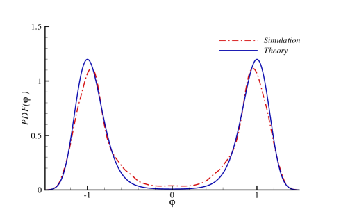
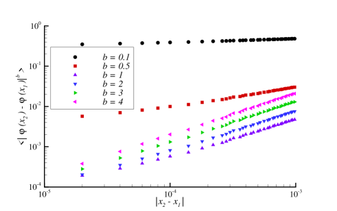
and the kicking period, $T=10^{-6}$. The number of collocation points chosen for our simulations is generally $N_{x}=10^{3}$. In Fig. 4 we plot the PDF of $\varphi$ according to Eq. (26), and compare it with the numerical results. In Fig. 5, the moments of $\varphi$ increments, $\langle|\varphi(x_{2}+\delta x)-\varphi(x_{1})|^{b}\rangle$, are calculated numerically as a function of $x=|x_{2}-x_{1}|$ for several values of $b$ (with $0<b<1$, and $1\leq b$) and its scaling exponents $\xi_{b}$ for $x<<1$ are checked. The results indicate that with good precision $\langle|\delta\varphi|^{b}\rangle$ scales with $x$ with an exponent $1$ for $b>1$; otherwise, it scales with $x$ with exponents $\xi_{b}=b$. Values of $\xi_{b}$ are given in Fig. 6.

The bi-fractal behavior of the exponents is a consequence of the presence of the domain walls. Indeed, the structure function,

$$C_{b}=\langle|\varphi(x_{2})-\varphi(x_{1})|^{b}\rangle\;,$$ (71)

for $b>0$ behaves, for small $\Delta x=|x_{2}-x_{1}|$ as,

$$C_{b}\sim A_{b}|\Delta x|^{b}+A^{\prime}_{b}|\Delta x|$$ (72)

where the first term is due to the regular (smooth) parts of the order parameter $\varphi$, while the second one is contributed by the $O(|\Delta x|)$ probability to have a domain wall somewhere in an interval of length $|\Delta x|$. For $0<b<1$ the first term dominates as $|\Delta x|\to 0$, while, for $b>1$ it is the second term that does so.

VI Summary

We studied the domain wall-type solutions in the $\varphi^{4}$-theory in the strong-coupling limit, $k^{\prime}\to 0$, in which the equation develops singularities. The scaling behavior of the moments of differences of $\varphi$, $\delta\varphi=\varphi(x_{2})-\varphi(x_{1})$, and the PDF of $\varphi$, i.e., $P(\varphi)$, were all determined. It was shown that in the stationary state, where the singularities are fully developed, the relaxation term in the strong-coupling limit leads to an unclosed term in the equation for the PDF. However, we showed that the unclosed term can be omitted in the strong-coupling limit. We proved that to leading order, when $|x_{2}-x_{1}|$ is small, fluctuation of the $\varphi$ field is intermittent for $b\geq 1$. The intermittency implies that, $C_{b}=\langle|\varphi(x_{1})-\varphi(x_{2})|^{b}>$ scales as $|x_{1}-x_{2}|^{\xi_{b}}$, where $\xi_{b}$ is a constant. It was shown, numerically, that for the space scale $|x_{2}-x_{1}|$ and $b\geq 1$, the exponents $\xi_{b}$ are equal to $1$.

VII APPENDIX I

In this appendix we provide a proof of Novikov’s theorem. Consider the general stochastic differential equation with the following form,

$$\frac{\partial}{\partial t}\varphi=-\frac{1}{2}L[\varphi(x,t)]+\eta(x,t)\;.$$ (73)

where $L$ is an operator acting on $\varphi$, and $\eta$ is a Gaussian noise with the correlation,

$$\langle\eta(x,t)\eta(x^{\prime},t^{\prime})\rangle=k(x-x^{\prime})\delta(t-t^{\prime})\;.$$ (74)

The PDF of the random noise has the following form,

$$[d\rho(\eta)]=[d\eta]\times$$ (75)

$$exp[-\frac{1}{2}\int d^{d}xd^{d}x^{\prime}dtdt^{\prime}\eta(x,t)B(x-x^{\prime})\delta(t-t^{\prime})\eta(x^{\prime},t^{\prime})]\;,$$ (76)

where $B(x-x^{\prime})$ is the inverse of $k(x-x^{\prime})$, so that,

$$\int k(x-x^{\prime})B(x^{\prime}-x^{\prime\prime})d^{d}x=\delta(x-x^{\prime\prime})\;.$$ (77)

we write the average of $\eta(x,t)F(\eta)$ over the noise realization as:

$$\langle\eta(x,t)F(\eta)\rangle=\int\eta(x,t)F(\eta)[d\rho(\eta)]\;.$$ (78)

By integrating by parts and using Eq. (77), one finds that,

$$\langle\eta(x,t)F(\eta)\rangle=$$ (79)

$$\int d^{d}x^{\prime\prime}dt^{\prime\prime}\langle\eta(x,t)\eta(x^{\prime\prime},t^{\prime\prime})\rangle\langle\frac{\partial F}{\partial\eta(x^{\prime\prime},t^{\prime\prime})}\rangle\;.$$ (80)

Now, let us assume the function $F$ to have the following form,

$$F[\eta]=exp(-i\lambda\varphi(x^{\prime},t))\;.$$ (81)

so that one finds,

$$\frac{\partial F}{\partial\eta(x^{\prime\prime},t^{\prime\prime})}=-i\lambda\frac{\partial\varphi(x^{\prime},t)}{\partial\eta(x^{\prime\prime},t^{\prime\prime})}F[\eta]\;,$$ (82)

Integrating Eq. (73) with respect to $t$, we find that,

$$\varphi(x^{\prime},t)=$$ (83)

$$\varphi(x^{\prime},t_{0})-\frac{1}{2}\int_{t_{0}}^{t}dt^{\prime\prime}L[\varphi(x^{\prime},t^{\prime\prime})]+\int_{t_{0}}^{t}dt^{\prime\prime}\eta(x^{\prime},t^{\prime\prime})\;.$$ (84)

This allows us to show that,

$$\frac{\partial\varphi(x^{\prime},t)}{\partial\eta(x^{\prime\prime},t^{\prime\prime})}=$$ (85)

$$-\frac{1}{2}\int_{t_{0}}^{t}dt^{\prime\prime\prime}\frac{\partial L[\varphi(x,t^{\prime\prime\prime})]}{\partial\eta(x^{\prime\prime},t^{\prime\prime})}+\delta(x^{\prime}-x^{\prime\prime})\theta(t-t^{\prime\prime})\;.$$ (86)

where, in the limit $t^{\prime\prime}\rightarrow t$, the first term of the right-hand side of Eq. (85) will vanish, and we can write

$$\langle\eta(x,t)\exp[-i\lambda\varphi(x^{\prime},t)]\rangle$$ (87)

$$=(-i\lambda)k(x-x^{\prime})\langle\exp(-i\lambda\varphi(x^{\prime},t))\rangle\;.$$ (88)

where we used, $\theta(0)=1$

VIII appendix II

In this Appendix we prove that, for example in Eq. (24), the relaxation term $k^{\prime}\nabla^{2}\varphi$ makes no contribution or anomaly to the PDF of the increments, in the limit $k^{\prime}\to 0$.

FIG. 5.: The moments, $\langle|\varphi(x_{2})-\varphi(x_{1})|^{b}\rangle$, as a function of $|x_{2}-x_{1}|$, obtained via numerical simulation.

FIG. 6.: Scaling exponents $\xi_{b}$, checked numerically. The results indicate that, with a good precision, $\langle|\delta\varphi|^{b}\rangle$ scales with $x$ with an exponent $1$ for $b>1$ larger than one, and elsewhere scales with $x$ with an exponent $\xi_{b}=b$.

The joint probability distribution $P(\varphi_{1},\varphi_{2})$ satisfies the following equation,

$$P_{t}(\varphi_{1},\varphi_{2})=-[(\varphi_{1}-\varphi_{1}^{3})P]_{\varphi_{1}}$$ (89)

$$-[(\varphi_{2}-\varphi_{2}^{3})P]_{\varphi_{2}}+k(0)(P_{\varphi_{1},\varphi_{1}}+P_{\varphi_{2},\varphi_{2}})$$ (90)

$$+2k(x)P_{\varphi_{1},\varphi_{2}}$$ (91)

$$-ik^{\prime}\int\frac{d\lambda_{1}}{2\pi}\frac{d\lambda_{2}}{2\pi}\lambda_{1}\exp(i\lambda_{1}\varphi_{1}+i\lambda_{2}\varphi_{2})$$ (92)

$$\times\langle\nabla^{2}\varphi(x_{1})\exp[-i\lambda_{1}\varphi(x_{1},t)-i\lambda_{2}\varphi(x_{2},t)]\rangle$$ (93)

$$-ik^{\prime}\int\frac{d\lambda_{1}}{2\pi}\frac{d\lambda_{2}}{2\pi}\lambda_{2}\exp(i\lambda_{1}\varphi_{1}+i\lambda_{2}\varphi_{2})$$ (94)

$$\times\langle\nabla^{2}\varphi(x_{2})\exp[-i\lambda_{1}\varphi(x_{1},t)-i\lambda_{2}\varphi(x_{2},t)]\rangle\;.$$ (95)

The last two terms in Eq. (47) are not closed with respect to the PDF. Let us then compute the contribution of the unclosed terms. They can be written as,

$$-ik^{{}^{\prime}}\int\frac{d\lambda_{1}}{2\pi}\frac{d\lambda_{2}}{2\pi}\lambda_{i}exp(i\lambda_{1}\varphi_{1}+i\lambda_{2}\varphi_{2})$$ (96)

$$\times<\nabla^{2}\varphi(x_{i})e^{-i\lambda_{1}\varphi(x_{1},t)-i\lambda_{2}\varphi(x_{2},t)}>$$ (97)

(98)

$$=-ik^{{}^{\prime}}(\int\frac{d\lambda_{1}}{2\pi}\frac{d\lambda_{2}}{2\pi}exp(i\lambda_{1}\varphi_{1}+i\lambda_{2}\varphi_{2})$$ (99)

$$\times<\nabla^{2}\varphi(x_{i})e^{-i\lambda_{1}\varphi(x_{1},t)-i\lambda_{2}\varphi(x_{2},t)}>)_{\varphi_{i}}$$ (100)

$$=-k^{\prime}\langle\nabla^{2}\varphi(x_{i})\delta(\varphi_{1}-\varphi(x_{1},t))$$ (101)

$$\times\delta(\varphi_{2}-\varphi(x_{2},t))\rangle_{\varphi_{i}}$$ (102)

Consider one of the terms in the above equation, for example, $-k^{\prime}\langle\nabla^{2}\varphi(x_{i})\delta[\varphi_{1}-\varphi(x_{1},t)]\times\delta[\varphi_{2}-\varphi(x_{2},t)]\rangle_{\varphi_{i}}$. Assuming ergodicity, it is written as,

$$=k^{\prime}\lim_{V\to\infty}\frac{1}{V}\int_{V}dx_{i}dv^{i}_{d-1}\nabla^{2}\varphi(x_{i})\delta[\varphi_{i}-\varphi(x_{i},t)]$$ (103)

in the limit, $k^{\prime}\to 0$ limit, only at the points where we have singularity this term is not zero. Therefore, we restrict ourselves to the space near the domain walls,

$$=-k^{\prime}\lim_{V\to\infty}\frac{1}{V}\sum_{j}\int_{\Omega_{j}}dx_{i}dv^{i}_{d-1}(\varphi_{x_{i}x_{i}}+\nabla^{2}_{d-1}\varphi)$$ (104)

$$\times\delta[\varphi_{i}-\varphi(x_{i},t)]$$ (105)

where $\Omega_{j}$ is the space close to the domain walls. Therefore, Eq. (52), in the limit, $k^{\prime}\to 0$, is written as,

$$=-k^{\prime}\lim_{V\to\infty}\frac{1}{V}\sum_{j}\int_{\Omega_{j}}dx_{i}dv^{i}_{d-1}\varphi_{x_{i}x_{i}}\delta[\varphi_{i}-\varphi(x_{i},t)]\;.$$ (106)

Changing the variables from $x_{i}$ to $z_{i}$ and integrating over $dv^{i}_{d-1}$, one finds,

$$=-k^{\prime}\lim_{V\to\infty}\frac{V_{d-1}}{V}\sum_{j}\int_{-\infty}^{+\infty}\epsilon dz_{i}\frac{1}{\epsilon^{2}}\varphi_{z_{i}z_{i}}\delta[\varphi_{i}-\varphi(z_{i},t)]$$

$$=-\frac{k^{\prime}}{\epsilon}\lim_{V\to\infty}\frac{V_{d-1}}{V}\sum_{j}\int_{-\infty}^{+\infty}dz_{i}\varphi_{z_{i}z_{i}}\delta[\varphi_{i}-\varphi(z_{i},t)]$$

where $\epsilon=(2k^{\prime})^{1/2}$. Assuming statistical homogeneity, we have

$$=-\frac{k^{\prime}}{\epsilon}\lim_{V\to\infty}\frac{NV_{d-1}}{V}\int_{-\infty}^{+\infty}dz_{i}\varphi_{z_{i}z_{i}}\delta[\varphi_{i}-\varphi(z_{i},t)]\\$$ (107)

where $N$ is number of singular lines. Moreover, $\frac{k^{\prime}}{\epsilon}=(k^{\prime})^{1/2}$, and, $\frac{NV_{d-1}}{V}$ is the density of the singular lines which, in the limit, $V\to\infty$, is simply the singularity density $\rho$. Therefore,

$$=-(k^{\prime})^{1/2}\rho\int_{-\infty}^{+\infty}dz_{i}\varphi_{z_{i}z_{i}}\delta[\varphi_{i}-\varphi(z_{i},t)]\;.$$ (108)

In the same way in, for example Eq. (21), by changing the integration variable from $z_{i}$ to $\varphi_{i}$, we calculate the integral exactly,

$$=\sqrt{k^{\prime}/2}\varphi\{A+2\sqrt{2}\phi_{i}^{2}\delta(\phi_{i}-1)\}$$

where $A=2\sqrt{2}\theta(1-\phi_{i}^{2})\theta(\phi_{i}^{2}-1)-\sqrt{2}\theta(1-\phi_{i}^{2})$. Therefore, in the limit, $k^{\prime}\to 0$ the master equation will give Eq. (35).

REFERENCES

- [1] K. G. Wilson, Phys. Rev. B 4, 3174, 3184 (1971); K. G. Wilson and M. E. Fisher, Phys. Rev. Lett. 28, 240 (1972); K. G. Wilson, ibid. 28, 548 (1972); A. A. Migdal, Sov. Phys. JETP 32, 552 (1971).
- [2] H. Kleinert and V. Schulte-Frohlinde, Critical Properties of -Theories (World Scientific, Singapore, 2001).
- [3] J. Berges and J. Cox, Phys. Lett. B 517, 369 (2001).
- [4] J. Berges, Nucl. Phys. A 699, 847 (2002).
- [5] K. Blagoev, F. Cooper, J. Dawson, and B. Mihaila, Phys. Rev. D 64, 125003 (2001).
- [6] G. Aarts, D. Ahrensmeier, R. Baier, J. Berges, and J. Serreau, Phys. Rev. D 66, 045008 (2002).
- [7] F. Cooper, J. F. Dawson, and B. Mihaila, Phys. Rev. D 67, 051901 (2003).
- [8] J. Berges and J. Serreau, hep-ph/0208070.
- [9] F. Cooper, J. F. Dawson, and B. Mihaila, Phys. Rev. D 67, 056003 (2003).
- [10] J. Baacke and A. Heinen, hep-ph/0212312.
- [11] J. Dreger, A. Pelster, and B. Hamperecht, Eur. Phys. J. B 45, 355 (2005).
- [12] A.-L. Barabasi and H. E. Stanley, Fractal Concepts in Surface Growth (Cambridge University Press, New York, 1995).
- [13] NATO Advanced Study Institute on Formation and Interactions of Topological Defects, edited by A.-C. Davis and R. Brandenberger (Plenum, New York, 1995).
- [14] L. P. Gorkov, Sov. Phys. JETP 9, 1364 (1959).
- [15] J. Bardeen, L. N. Cooper, J. R. Schrieffer, Phys. Rev. 108, 1175 (1957).
- [16] V. L. Ginzburg and L. D. Landau, Zh. Eksp. Teor. Fiz. 20 1064 (1950); reprinted in L. D. Landau, Collected Papers (Pergamon, London, 1965), p. 546.
- [17] A. Schmid, Z. Phys. 215, 210 (1968).
- [18] L. P. Gorkov and G. M. Eliashberg, Sov. Phys. JETP 27, 338 (1968).
- [19] A. C. Newell and J. A. Whitehead, J. Fluid Mech. 38, 279 (1969).
- [20] L. A. Segel, J. Fluid Mech. 38, 203 (1969).
- [21] P. C. Hohenberg and B. I. Halperin, Rev. Mod. Phys. 49, 435 (1977).
- [22] C. M. Bender and S. A. Orzag,Advanced Mathematical Methods for Scientists and Engineers, 3rd International Edition (McGraw-Hill, New York, 1987).
- [23] A. A. Masoudi, F. Shahbazi, J. Davoudi and M. R. Rahimi Tabar, Phys. Rev. E 65 026132 (2002).
- [24] H. Risken, The Fokker-Planck equation, Springer-Verlag Berlin, 1984.
- [25] U. Frisch and J. Bec, in Les Houches 2000: New Trends in Turbulence, edited by M. Lesieur, A. Yaglom, and F. David (Springer EDP-Sciences, Berlin, 2001), p. 341.
- [26] R. Peyret, Computational Fluid Mechanics (Academic Press, San Diego, 2000).
- [27] R. W. Hockney and J. W. Eastwood, Computer Simulation Using Particles (Institute of Physics Publishing, London, 1992).
- [28] J. Bec, U. Frisch, and K. Khanin, J. Fluid Mech. 416, 239 (2000).