Devil’s staircases, quantum dimer models, and stripe formation in strong coupling models of quantum frustration

Abstract

We construct a two-dimensional microscopic model of interacting quantum dimers that displays an infinite number of periodic striped phases in its $T=0$ phase diagram. The phases form an incomplete devil’s staircase and the period becomes arbitrarily large as the staircase is traversed. The Hamiltonian has purely short-range interactions, does not break any symmetries of the underlying square lattice, and is generic in that it does not involve the fine-tuning of a large number of parameters. Our model, a quantum mechanical analog of the Pokrovsky-Talapov model of fluctuating domain walls in two dimensional classical statistical mechanics, provides a mechanism by which striped phases with periods large compared to the lattice spacing can, in principle, form in frustrated quantum magnetic systems with only short-ranged interactions and no explicitly broken symmetries.

I Introduction

The past two decades have seen the discovery of a number of strongly correlated materials with unconventional physical properties. Due to the competing effects of essentially electronic processes and interactions these doped Mott insulators typically exhibit complex phase diagrams which include antiferromagnetic phases, generally incommensurate charge-ordered phases, and high temperature superconducting phases. When conducting, these systems do not have well defined electron-like quasiparticles and their metallic states thus cannot be explained by the conventional theory of metals, the Landau theory of the Fermi liquid, and the associated superconducting states cannot be described in terms of the BCS mechanism for superconductivity.

The startling properties of these materials have led to a number of proposals of non-trivial ground states of strongly correlated systems which share the common feature that they cannot be adiabatically obtained from the physics of non-interacting electrons. A class of proposed ground states are the resonating valence bond (RVB) spin liquid phases, quantum liquid ground states in which there is no long range spin order of any kind, and the related valence bond crystal phases, of frustrated quantum antiferromagnetsAnderson (1987); Kivelson et al. (1987) and their descendants.Lee et al. (2006); Senthil and Fisher (2000); Hermele et al. (2005); Mudry and Fradkin (1994) On the other hand, the presence of competing spatially-inhomogeneous charge-ordered phases in close proximity to both antiferromagnetism and high $T_{c}$ superconductivity, and the existence of incommensurate low energy fluctuations in the latter phase, strongly suggest that these phases may have a common origin. It has long been suggested that some form of frustration of the charge degrees of freedom may be at work in these systems.Emery and Kivelson (1993); Emery et al. (1999); Kivelson et al. (1998) The explanation of both the existence of a large pairing scale in the superconducting phase and their close proximity to inhomogeneous charge-ordered phases is one of the central conceptual challenges in the physics of these doped Mott insulators.Kivelson and Fradkin (2006)

The most studied class of these strongly correlated materials are the cuprate high temperature superconductors (for a recent review on their behavior and open questions see Ref. Kivelson et al., 2003.) Unconventional behaviors have also been seen in other strongly correlated complex oxides.Mackenzie and Maeno (2003) More recently, strong evidence for non-magnetic phases has been discovered in new frustrated quantum magnetic materials, including the quasi-2D triangular antiferromagnetic insulators such asColdea et al. (2001) Cs₂CuCl₄, the quasi-2D triangular organic compounds such asShimizu et al. (2003) $\kappa$-(BEDT-TTF)₂Cu₂(CN)₃, and the 3D pyrochlore antiferromagnets such as the spin-ice compoundRamirez et al. (1999); Snyder et al. (2004) Dy₂Ti₂O₇ (although quantum effects do not appear to be prominent in spin-ice systems.)

It is thus of interest to develop a theoretical framework to describe quantum frustrated systems in the regime of strong correlation, and to understand their role in the mechanism for inhomogeneous phases in strongly correlated systems. This is the main purpose of this paper. It has long been known that generally incommensurate inhomogeneous phases arise in classical systems with competing short range attractive interactions and long range repulsive interactions. In such systems, the short range attractive interactions (whose physical origin depend on the system in question) favor spatially inhomogeneous phases, i.e. phase separation, which is frustrated by long range (typically Coulomb) repulsive interactions. Coulomb-frustrated phase separation has been proposed as a mechanism for stripe phases in doped Mott insulatorsEmery and Kivelson (1993); Löw et al. (1994); Lorenzana et al. (2001) and in low density electron gases.Jamei et al. (2005) Similar ideas were also proposed to explain the structure of the crust of neutron stars, lightly doped with protons,Ravenhall et al. (1983); Lorenz et al. (1993) and in soft condensed matter (e.g. block copolymers).Seul and Andelman (1995)

In this work we will pursue a different approach and consider mechanisms of quantum stabilization (i.e. quantum order by disorder) of stripe-like phases in frustrated quantum systems. We will specifically consider frustrated versions of two-dimensional quantum dimer models,Rokhsar and Kivelson (1988) which provide a qualitative description of the physics of quantum frustrated magnets in their spin-disordered phases. The phases that we will discuss here are essentially valence bond crystals with varying degree of commensurability and become asymptotically incommensurate. Since these systems are charge-neutral, there are no long range interactions. As we will see below, quantum fluctuations resolve the high degeneracies of their naive classical limit leading to a non-trivial phase diagram with phases with different degree of commensurability or tilt. The resulting phase diagram has the structure of an incomplete devil’s staircase similar to that found in classical order-by-disorder systems such as the anisotropic next-nearest neighbor Ising (ANNNI) modelsFisher and Selke (1980); Bak (1982). In the regime in which quantum fluctuations are weak, which is where our calculations are systematically controlled, only a small fraction of the phase diagram exhibits phases with non-trivial modulations. In this “classical” regime the observation of non-trivial phases requires fine tuning of the coupling constants. (In contrast, in systems with long range interactions no such fine tuning is needed at the classical level.Löw et al. (1994)) However, as the quantum fluctuations grow, the fraction of the phase diagram occupied by these non-trivial phases becomes larger. Thus, at finite values of the coupling constants, where our estimates are not accurate, no fine tuning is needed.

Considerable progress has been made towards understanding theoretically the liquid phases, including the proper field theoretic descriptionMoessner et al. (2002); Ardonne et al. (2004) which also allows for an analysis of the related valence bond solid phases with varying degrees of commensurability.Vishwanath et al. (2004); Fradkin et al. (2004) Complementary to this effort is the dynamical question of how, or even if, a phase with exotic non-local properties can arise in a system where the interactions are purely local. We emphasize the requirement of locality because many of these exotic structures have been proposed for experimental systems believed to be described by a local Hamiltonian (i. e. of the Hubbard or Heisenberg type). An additional question is whether the exotic physics can be realized in an isotropic model or if it is necessary for the Hamiltonian to explicitly break symmetries. For some of these structures, the dynamical questions have been partially settled by the discovery of model HamiltoniansMoessner and Sondhi (2001); Kitaev (2006); Ardonne et al. (2004) which stabilize the exotic phase over a portion of their quantum phase diagrams. While many of these models do not (currently) have experimental realizations, their value, in addition to providing proofs of principle, lies in the identification of physical mechanisms, which often have validity beyond the specific case considered. For example, the existence of short-range RVB phases was first demonstrated analytically in quantum dimer modelsRokhsar and Kivelson (1988); Moessner and Sondhi (2001), the essential ingredients being geometric frustration and ring interactions. The possibility of such phases being realized in spin systems was subsequently demonstrated by the construction of a number of spin HamiltoniansHermele et al. (2004); Balents et al. (2002); Fujimoto (2005); Raman et al. (2005); Damle and Senthil (2006); Isakov et al. (2006); Sengupta et al. (2006), including SU(2) invariant modelsFujimoto (2005); Raman et al. (2005), all of which reduce to dimer-like models at low energies. The existence of commensurate valence bond solid phases, with low order commensurability, in doped quantum dimer modelsFradkin and Kivelson (1990) has been studied recentlyBalents et al. (2005a, b), as well as modulated phases in doped quantum dimer models within mean field theory.Vojta and Sachdev (1999)

It is in this context that we ask the following question: is it possible to realize high order striped phases in a strongly-correlated quantum system with only local interactions and no explicitly broken symmetries? While the term stripe has been used in reference to a number of spatially inhomogeous states, here we use the term to denote a domain wall between two uniform regions. The presence of domain walls means that rotational symmetry has been broken. Fig. 1 gives examples of striped phases. Theories based on the formation of striped phases have been proposed in a number of experimental contexts, notably the high $T_{c}$ cupratesZaanen and Gunnarsson (1989); Zhang and Henley (2003); Vojta and Sachdev (1999); Kivelson et al. (1998), where the “stripes” are lines of doped holes separating antiferromagnetic domains (see Fig. 1a). In the simplest striped states, the domain walls are periodically spaced (Fig. 1b) or are part of a repeating unit cell (Fig. 1c). We use the term “high order striped phase” in the case where the periodicity is large compared to the other characteristic lengths in the model.

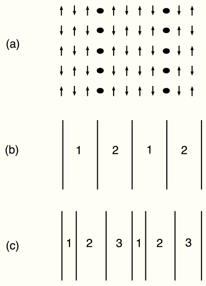
Figure 1: Examples of striped phases. (a) shows stripes of holes separating antiferromagnetic domains. This structure appears in some theories of the high $T_{c}$ cuprates. (b) shows periodically spaced domain walls separating regions where the order parameter takes the uniform value $\phi_{1}$ or $\phi_{2}$. (c) is another example where the periodicity is associated with a repeating unit cell. If the repeat distance becomes infinite, then the state is said to be incommensurate with the lattice.

Our central result is a positive answer to the question posed in the preceding paragraph. We do this by constructing a two-dimensional quantum dimer model, with only short range interactions and no explicitly broken symmetries, that shows an infinite number of periodic striped phases in its $T=0$ phase diagram. The collection of states forms an incomplete devil’s staircase. The phases are separated by first order transitions and the spacing between stripes becomes arbitrarily large as the staircase is traversed.

Before giving details of the construction, we reiterate that we are searching for (high-order) striped phases in a Hamiltonian with only local interactions and without explicitly breaking any symmetries. As alluded to earlier, a number of experimental systems where stripe-based theories have been proposed are widely believed to be described by Hamiltonians that meet these restrictions. A notable example is the Emery model Emery (1987); Kivelson et al. (2004) of the high-$T_{c}$ cuprates, which is a generalization of the Hubbard model that includes both Cu and O sites. Since it is not a priori obvious that a nontrivial global ordering such as a high order striped phase will/can unambiguously arise from such local, symmetric strongly correlated models, we include these phases in the list of “exotic” structures. However, in the absence of these restrictions, the occurrence of stripe-like phases is relatively common. Relaxing the requirement of high periodicity, we note that low order striped quantum phases can occur in the Bose-Hubbard model at fractional fillings if appropriate next-nearest-neighbor interactions are addedBalents et al. (2004). Relaxing the requirement of locality, we note that stripe phases arise naturally in systems with long range Coulomb interactionsVojta and Sachdev (1999); Jamei et al. (2005). More generally, if the Hamiltonian includes a term that is effectively a chemical potential for domain walls, and if there is a long-range repulsive interaction between domain walls, then we may generically expect striped phases where the spacing between domain walls is large (compared with the lattice spacing).

A guiding principle in constructing models with exotic phases is frustration, or the inability of a system to simultaneously optimize all of its local interactions. Quantum dimer models are relatively simple models that contain the basic physics of quantum frustration and have proven to be a useful place to look in the search for exotic phasesMoessner and Sondhi (2001). This is one reason why we choose to work in the dimer Hilbert space. A second reason is related to the observation that each dimer covering may be assigned a winding number and this divides the Hilbert space into topological sectors that are not coupled by local dynamics. The ground state wavefunction of a dimer Hamiltonian will typically live in one of these sectors (ignoring the complications of degeneracy for the moment). As parameters in the Hamiltonian are varied, it is possible that at some critical value, the sector containing the ground state will change. Such a scenario, which occurs even in the simplest dimer model formed by Rokhsar and Kivelson, is an example of a quantum tilting transition between a “flat” and “tilted” state. In Refs. Vishwanath et al., 2004 and Fradkin et al., 2004, it was shown, by field theoretic arguments, that when such a transition is perturbed, states of “intermediate tilt” (this will be made more precise below) may be stabilized. As we will show, these intermediate tilt states may be viewed as stripe-like states, of the form we are interested in. Taking inspiration from these ideas, our construction involves perturbing about a tilting transition in a specially constructed dimer model.

In classical Ising systems, the competition between nearest-neighbor and next-nearest-neighbor interactions is a well-known mechanism for generating incommensurate phases Fisher and Selke (1980). Classical models of striped phases are based on two complementary principles: soliton formation and competing interactionsBak (1982). Our quantum construction is based on analogies with two classical models that are representatives of these two aspects: the Pokrovsky-Talapov model of fluctuating domain wallsPokrovsky and Talapov (1978) and the ANNNI modelFisher and Selke (1980). In section II, we review the relevant features of these models. In section III, we review the salient features about dimer models and tilting transitions. In section IV, we give an overview of the construction and technical details are presented in section V and the appendices. In section VI, we discuss how these ideas connect to spin models, thus extending our “proof of principle” to systems with physical degrees of freedom. We discuss implications of these results in section VII. In two appendices we give technical details of our calculations.

II Classical models

Our approach builds on principles underlying stripe formation in classical models, where the problem is also referred to as a commensurate-incommensurate transitionBak (1982). The classical models are based on two complementary principles: the insertion of domain walls and competing local interactions.

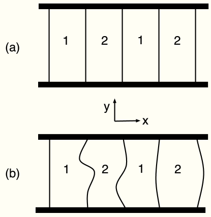
Figure 2: (a) ground and (b) excited states of the Pokrovsky-Talapov model of fluctuating classical domain walls. This is a two-dimensional anisotropic model where domain walls form along the $y$ direction and separate regions where the order parameter is uniform. While the domain walls cost energy, they are allowed to fluctuate, which carries entropy. For a range of parameters, the domain walls are actually favored by the free energy minimization.

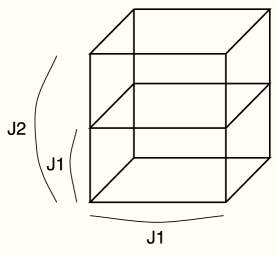
Figure 3: The anisotropic next nearest neighbor Ising (ANNNI) model. Ising spins lie on the points of a $d$-dimensional cube. Nearest neighbor interactions are ferromagnetic ($J_{1}<0$. Along one of the directions, we also have antiferromagnetic next nearest neighbor interactions $J_{2}>0$.

A toy model relevant to the present work is the picture of fluctuating domain walls in two dimensions, introduced by Pokrovsky and TalapovPokrovsky and Talapov (1978). The walls are allowed to fluctuate though the ends are fixed (Fig. 2), which precludes bubbles. The free energy minimization is a competition between the creation energy of having walls, the elastic energy of deviating from the flat state, and the entropic benefit of allowing the walls to fluctuate. This theory predicts a transition from a uniform phase to a striped phase. The spacing between walls depends on the parameters of the theory (including temperature) and can be large compared with other length scales.

A second model relevant to the present work is the classical anisotropic next-nearest-neighbor Ising (ANNNI) model in three (and higher) dimensionsFisher and Selke (1980); Bak and von Boehm (1980). This model (Fig. 3) describes Ising spins on a cubic lattice with ferromagnetic nearest-neighbor interactions $J_{1}<0$ and antiferromagnetic next-nearest-neighbor interactions $J_{2}>0$ along one of the lattice directions. A key feature of the ANNNI Hamiltonian is a special point $J_{1}/J_{2}=2$ where a large number of stripe-like states are degenerate at zero temperature. As the temperature is raised, the competition between $J_{1}$ and $J_{2}$ causes an infinite number of modulated phases to emerge from this degenerate point. The phase diagram in the low $T$ limit was studied analytically in Ref. Fisher and Selke, 1980 using a novel perturbative scheme where the existence of higher order phases was established at successively high orders in the perturbation theory. Numerical studies at higher temperaturesBak and von Boehm (1980) indicated that incommensurate phases occur near the phase boundaries. Therefore, the collection of phases form an incomplete devil’s staircaseBak (1982); 3da . A quantum version of the ANNNI model was studied in Refs. Harris et al., 1995a and Harris et al., 1995b.

The phase diagram of our model is similar to that of the ANNNI model and our analytical methods are similar in spirit to Ref. Fisher and Selke, 1980. However, the basic physics of our model corresponds more clearly to a quantum version of the energy-entropy balance occuring in the fluctuating domain wall picture. We now discuss one more ingredient of the construction before putting the pieces together in section IV.

III Quantum dimer models and tilting transitions

A hard-core dimer covering of a lattice is a mapping where each site of the lattice forms a bond with exactly one of its nearest neighbors. Each dimer covering is a basis vector in a dimer Hilbert space and the inner product is such that different dimer coverings are orthogonal. Quantum dimer models are defined on this dimer Hilbert space through operators that manipulate these dimers in ways that preserve the hard-core condition. These models were first proposed as effective descriptions of the strong coupling regime of quantum spin systemsRokhsar and Kivelson (1988) and Refs. Balents et al., 2002; Fujimoto, 2005; Raman et al., 2005 discuss ways in which this correspondence can be made precise.

The space of dimer coverings can be subdivided into different topological sectors labelled by the pair of winding numbers $(W_{x},W_{y})$ defined in Fig. 4. The winding number is a global property in that it is not affected by any local rearrangement of dimers. In particular, for any local Hamiltonian, the matrix element between dimer coverings in different sectors will be zero.

For a given local Hamiltonian, the ground state of the system will typically lie in one of the topological sectors. A common occurrence in dimer models is a quantum phase transition in which the topological sector containing the ground state changes. Such an occurrence is called a tilting transition because a dimer covering of a 2d bipartite lattice may be viewed as the surface of a three-dimensional crystal through the height representationBlöte and Hilhorst (1982). In this language, the different topological sectors correspond to different values for the (global) average tilt of the surface. The correspondence between dimers and heights is reviewed in Fig. 5 but for the present purpose, it is sufficient to define the “tilt” of a dimer covering as its “winding number per unit length”. The simplest dimer model introduced in Ref. Rokhsar and Kivelson, 1988, has a tilting transition between a flat state (zero tilt) and the staggered state, which is maximally tilted (Fig. 5b). At the critical point, called the Rokhsar-Kivelson or RK point, the Hamiltonian has a ground state degeneracy where all tilts are equally favored.

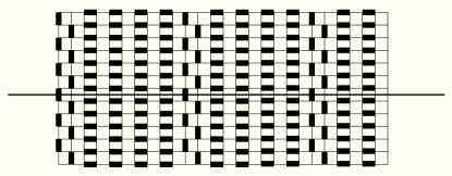
Figure 4: Winding numbers: draw a reference line that extends through and around (due to the periodic boundary condition) the system and label the vertical lines of the lattice alternately as $A$ and $B$ lines. For any dimer configuration, we may define, with regard to this reference line, the winding number $W_{x}=N_{A}-N_{B}$, where $N_{A}$ is the number of $A$ dimers intersecting the line and similarly for $N_{B}$. We can similarly draw a vertical line and define a similar quantity $W_{y}$. Note that this particular construction works for a 2d bipartite lattice. For 2d non-bipartite lattices, the construction is simpler: count the total number of dimers intersecting the horizontal and vertical reference lines and there are four sectors corresponding to whether $W_{x,y}$ is even or odd.

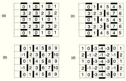
Figure 5: Sample dimer configurations with corresponding height mappings. The height mapping involves assigning integers to the squares of the lattice in the following manner. Divide the bipartite lattice into $A$ and $B$ sublattices. Assign zero height to a reference square and then moving clockwise around an $A$ site, the height increases by one if a dimer is not crossed and decreases by three if a dimer is crossed. The same rule applies moving counterclockwise about a $B$ site. The integers correspond to local heights of a crystal whose base lies on the page. In these examples, the lower square in the second column is taken as the reference square. (a) Dimers are arranged in columns corresponding to a surface that is flat on average (though there are fluctuations at the lattice scale). (b) Dimers are staggered and the corresponding surface is maximally tilted. (c) There average tilt is nonzero due to the staggered strip in between the flat columnar regions. (d) Going from left to right, the surface initially falls and then rises giving an average tilt of zero. This is because the two staggered regions have opposite orientation.

The recognition of the Rokhsar-Kivelson dimer model as a tilting transition led to a field theoretic description Henley (1997); Moessner et al. (2002) of the RK point based on a coarse-grainedact version of the height field (Fig. 5). The stability of this field theory was studied in Refs. Vishwanath et al., 2004 and Fradkin et al., 2004. These studies showed that by tuning a small perturbation and non-perturbatively adding irrelevant operators, it is possible to make the tilt vary continuously from a flat state to the maximally tilted state. In addition, it was observed that the system has a tendency to “lock-in” at values of the tilt commensurate with the underlying microscopic lattice, the specific values depending on details of the perturbation. It was also noted that while a generic perturbation would make the transition first orderVishwanath et al. (2004), for a sufficiently small perturbation, the correlation length was extremely largeFradkin et al. (2004) which, it was argued, justified the field theory approach nonetheless. Therefore, the generic effect of perturbations would be to smoothen the Rokhsar-Kivelson tilting transition by making the system pass through an incomplete devil’s staircase of intermediately tilted states. One may suspect that the structure of the field theory, including the predictions of Refs. Vishwanath et al., 2004 and Fradkin et al., 2004, would hold for a broader class of tilting transitions. In particular, one may consider the case where the critical point is merely a point of large degeneracy where all tilts are favoredtil ; nus , which is analogous to the classical ANNNI model.

The relevance of all of this to the present work is most easily seen by Fig. 9, which shows the simplest examples of states that have intermediate tilt (i. e. winding number). These are stripe-like states having a finite density of staggered domain walls and more general tilted states may be obtained by locally rearranging the dimers. The preceding discussion suggests that these kinds of structures arise naturally when quantum dimer models are perturbed around a tilting transition. This observation will guide the construction outlined in the next section.

IV Overview of strategy

We now combine various ideas presented in sections II and III to construct the promised quantum model. In the present section, we present an overview of the construction with details and subtleties relegated to section V. The basic idea is to construct a quantum dimer model with a tilting transition and then to appropriately perturb this model to realize a staircase of striped states. We design the unperturbed system to have a large degeneracy at the critical point, with each of the degenerate states having a domain-wall structure. The perturbation will effectively make these domain walls fluctuate and the degeneracy will be lifted in a quantum analog of the energy-entropy competition that drives the classical Pokrovsky-Talapov transition. Using standard quantum mechanical perturbation theory, we will obtain a phase diagram similar to the classical 3D ANNNI model and will find that phases with increasingly long periodicities will be stabilized at higher orders in the perturbation theory. This mathematical approach is similar in spirit to the analysis of the classical ANNNI model in Ref. Fisher and Selke, 1980.

A simple, rotationally invariant Hamiltonian with a tilting transition is given by:

This model displays a first-order transition between a columnar and fully staggered state at a very degenerate point, where $2a=b$. In principle, we may perturb this model with an off-diagonal resonance term and expect phases with intermediate tilt (and possibly other exotic phases) on the general grounds discussed in the previous section. However, it is difficult to make precise statements about the phase diagram even for such fairly simple models. We will study a slightly constrained version of this model that is convenient for making analytical progress.

We construct the quantum dimer model in two steps. First, we construct a diagonal parent Hamiltonian $H_{0}$ (Eq. 3) where the ground states are separated from excited states by a tunably large gap. $H_{0}$ will not break any lattice symmetries, but the preferred ground states will spontaneously break translational and rotational symmetry. In particular, we design $H_{0}$ to select ground states having the domain wall structure shown in Fig. 6. In these states, the dimers arrange themselves into staggered domains of unit width separating columnar regions of arbitrary width. The columnar dimers are horizontal if the staggered dimers are vertical (and vice versa) and the staggered strips come in two orientations. Notice that the fully columnar state (a columnar region of infinite width) is included this collection but the fully staggered state (Fig. 5b), which appears in the Rokhsar-Kivelson phase diagram, is not. In the following, we will typically draw the staggered strips as vertical domain walls but the horizontal configurations are equally possible.

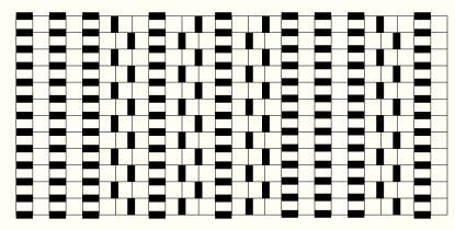
Figure 6: A typical domain wall state selected by $H_{0}$. These states break translational and rotational symmetry. The staggered strips, which are one column wide and may have one of two orientations, are like domain walls separating columnar regions, which may have arbitrary width. When $a=b$ in Eq.  4, the set of these states spans the degenerate ground state manifold of $H_{0}$.

In analogy with the ANNNI model, $H_{0}$ is designed so that all of these domain wall states are degenerate when the couplings are tuned to a special point. Away from this point, the system will enter either a flat or a tilted phase. The unperturbed phase diagram is sketched in Fig. 7.

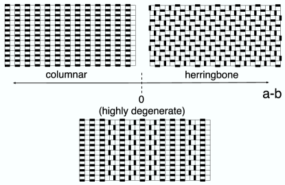
Figure 7: Ground state phase diagram of the parent Hamiltonian $H_{0}$ as a function of the parameter $a-b$ (see Eq. 3). In these states, the dimers may only have two attractive bonds. When $a-b=0$, the states of Fig. 6 are degenerate ground states. Away from this point, the system enters a state where dimers either maximize or minimize the number of staggered interactions. The maximally staggered configuration is commonly called the “herringbone” state.

The second step of the construction is to perturbatively add a small, non-diagonal, resonance term $tV$:

The sum is over all plaquettes in the lattice. Depending on the local dimer configuration of the wavefunction, the individual terms in this sum will either annihilate the state or flip the local cluster of dimers as shown in Fig. 8. The action of this operator on the domain wall states (Fig. 6) is confined to the boundaries between staggered and columnar regions and effectively makes the domain walls fluctuate. Notice that Eq. 2 is equivalent to two actions of the familiar Rokhsar-Kivelson two-dimer resonance term. We expect the basic conceptual argument to apply for a more general class of perturbations, including the two-dimer resonance, but we consider the specific form of Eq. 2 to simplify certain technical aspects of the calculation. We will elaborate on this more in the next section.

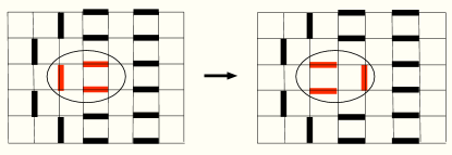
Figure 8: One of the terms in the operator of Eq. 2 will flip the circled cluster as shown.

The degenerate point of Fig. 7 may be viewed as the degeneracy of an individual vertical column having a staggered or columnar dimer arrangement. The perturbation 2 lifts this degeneracy by lowering the energy of configurations with domain walls by an amount of order $\sim Lt^{2}$ per domain wall, where $L$ is the linear size of the system. Therefore, the system favors one of the states with a maximal number of domain walls and for technical reasons discussed below, will choose the one having maximal tilt: the [11] state in Fig. 9a. However, the degeneracy between columnar and staggered strips will be restored by detuning $H_{0}$ from the $t=0$ degenerate point. This implies the second order phase diagram sketched in Fig. 10.

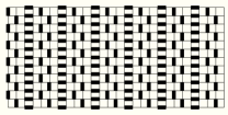
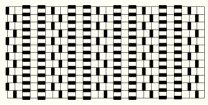
(a)	(b)
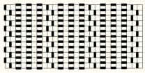
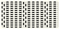
(c)	(d)
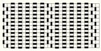
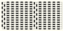
(e)	(f)

Figure 9: Examples of ideal tilted states. In these states, the domain walls have the same orientations and are uniformly spaced. The notation [1n] denotes the state where one staggered strip is followed by $n$ columnar strips and so on. It is understood that [1n] collectively refers to the above states and those related by translational, rotational, and reflection (i.e. switching the orientation of the staggering) symmetries. The examples drawn here, where it is understood that what we are seeing is part of a larger lattice, are (a) [11] (b) [12] (c) [13] (d) [14] (e) [15] (f) [16].

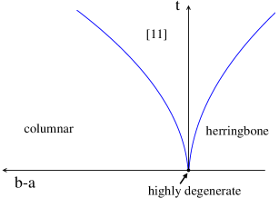
Figure 10: (Color online) Ground state phase diagram of $H=H_{0}+tV$ from second order perturbation theory.

Fig. 10 is correct up to error terms of order $t^{4}$. To this approximation, states having tilt in between the [11] state and the (flat) columnar state are degenerate on the phase boundary. Physically, this boundary occurs when the energy from second order processes which stabilize the staggered domains is precisely balanced by the energy of a columnar strip. This degeneracy will be partially lifted by going to higher orders in perturbation theory. We find that at fourth order, a new phase is stabilized in a region of width $\sim t^{4}$ between the columnar and [11] phases. This new phase is the one which maximizes the number of fourth order resonances shown in Fig. 11 and is the [12] state (Fig. 9b). The corrected phase diagram is given in Fig. 12.

Figure 11: (Color online) The excited state on the right is obtained from the initial state by acting twice with the perturbation in Eq. 2.

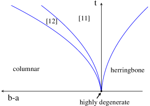
Figure 12: (Color online) Ground state phase diagram of $H=H_{0}+tV$ from fourth order perturbation theory. The width of the [12] phase is order $t^{4}$.

Fig. 12 is accurate up to corrections of order $t^{6}$. To this approximation, on the boundaries, states with tilts in between the bordering phases are degenerate. These degeneracies will be partially lifted at higher orders in the perturbation. At higher orders, there will be resonances corresponding to increasingly complicated fluctuations of the staggered lines but at $n$th order, the competition between the [1,n-1] and columnar phases will always be decided by the $n$th order generalization of the long resonance in Fig. 11. The competition will stabilize a new [1n] phase in a tiny region of width $\sim t^{2n}$ between the [1,n-1] and columnar phases resulting in the phase diagram of Fig. 13.

%

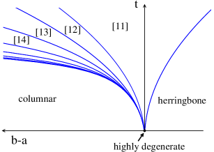
Figure 13: (Color online) Ground state phase diagram of $H=H_{0}+tV$ from nth order perturbation theory. The width of the [1n] phase is of order $t^{2n}$.

%

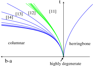
Figure 14: (Color online) The boundaries of the [1n] sequence will typically open into finer phases and subsequently the fine boundaries can themselves open. While the detailed structure depends on parameters in the model, generically we expect an incomplete devil’s staircase to be realized. In the figure,we have explicitly drawn the opening of the[11]-[12] boundary but the other boundaries will behave similarly.

We will also find that at higher orders, the individual boundaries of the [1n] sequence will themselves open revealing finer phase boundaries, which themselves can open. This leads to the generic phase diagram sketched in Fig. 14. The steps in the [1n] sequence that are stabilized depend on the values of parameters in the Hamiltonian. However, the conclusion of arbitrarily long periods being realized is robust. The fine structure of how the [1,n-1]-[1n] boundaries open is less certain because the dependence on parameters is more intricate and increasingly complicated resonances need to be accounted for. However, general arguments indicate that the boundaries will open and even periods incommensurate with the latticefoo (a) are likely to occur in the model, though such states will not be seen at any finite order of our perturbation theory.

In the terminology of commensurate-incommensurate phase transitions, the [1n] sequence forms a (harmless) staircase with a “devil’s top-step”Fisher and Selke (1980); Bak (1982). With the openings of these boundaries, beginning in the [11] state and moving left in Fig. 14 for $t\neq 0$, the system traverses an incomplete devil’s staircase of periodic states. The subsequent steps in the staircase have progressively smaller tilts culminating in the flat columnar state. The phase boundaries are first order transitions. This phase diagram is similar to what is seen in the classical ANNNI model, where the transitions are driven by thermal fluctuations.

We make two remarks before launching into the calculation. First, when we refer to the “[11] phase” (for example) what we precisely mean is that in this region, the ground state wavefunction is a superposition of dimer coverings that has relatively large overlap with the state in Fig. 9a and much smaller overlaps (of order $t^{2}$, $t^{4}$ etc. ) with excited states obtained by acting on Fig. 9a with Eq. 2. The coefficients follow from perturbation theory. Second, since Fig. 14 is obtained using perturbation theory, we can be confident that this describes our system only in the limit where $t$ is small. In the classical ANNNI model, numerical evidence indicates that as the small parameter (the temperature in that case) is increased, the phase boundaries close into Arnold tongue structures. We do not currently know if this will occur in our model as $t$ increases.

V Details

In this section, we construct a Hamiltonian using the strategy outlined in the previous sections. The Hamiltonian $H=H_{0}+tV$ consists of a diagonal term $H_{0}$ and an off-diagonal term $tV$, which we treat perturbatively in the small parameter $t$.

V.1 Parent Hamiltonian

Our parent Hamiltonian $H_{0}$ is the following operator:

The coefficients $a$, $b$, $c$, $d$, $p$, and $q$ are positive numbers. The symbols used in Eq. 3 are projection operators referring to configurations of dimers on clusters of plaquettes and the sums are over all such clusters. The notation “3 more”, etc. refers to the given term as well terms related to it by rotational and/or reflection symmetry; in terms $a$ and $b$ these other terms are explicitly written. Notice that this Hamiltonian is a sum of local operators and does not break any symmetries of the underlying square lattice.

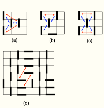
Figure 15: (Color online) (a) and (b) are the two ways in which a dimer can participate in three attractive bonds. (c) is the one way in which a dimer can participate in four attractive bonds. The attractive bonds are shown by the blue (dark gray) arrows. However, these configurations also involve repulsive interactions, which are shown in red (light gray), from terms $c$ and $d$ in the Hamiltonian. (d) is an example of a state where every where every dimer has only two attractive bonds but with some dimers the two bonds are of different types. These “kinks” in the staggered domain walls involve an energy cost from term $d$ as indicated by the red (light gray) arrows.

Terms $a$ and $b$ are attractive interactions favoring staggered and columnar dimer arrangements respectively and we study Eq. 3 near $a=b$. Terms $c$ and $d$ are repulsive interactions and if $c,d\geq a,b$, the dimers prefer domain wall patterns (Fig. 6). Terms $p$ and $q$ are repulsive interactions which determine the phases on the staircase. If these terms are sufficiently largeinf compared to $a,b,c$ and $d$, the staircase will include phases with arbitrarily long periods.

We begin by showing that when $a=b$, the ground states of $H_{0}$ are the domain wall states of Fig. 6. We do this by showing that competitive states must have higher energy. In the domain wall states, every dimer participates in exactly two attractive interactions and no repulsive interactions. The only way to achieve a lower energy is for some dimers to participate in three or four attractive interactions. This involves local dimer patterns of the form shown in Fig. 15abc. In Fig. 15a, the central dimer participates in one columnar and two staggered interactions but also two repulsive interactions from term $d$ in Eq. 3. Similarly, Figs. 15b and 15c show that if a dimer participates in more than two staggered interactions, the extra bonds are penalized by term $c$. If we require $c,d\geq a,b$, these patterns will result in higher energy states as the repulsive terms nullify the advantage of having extra attractive bonds. This also explains why in Fig. 6, the staggered strips have unit width and the staggered and columnar dimers have opposite orientation.

Of the states where every dimer has two attractive bonds, the states where some dimers have two bonds of different type will also have higher energy as shown in Fig. 15d. Of the remaining states, it is readily seen that states where every dimer participates in either two $a$ bonds or two $b$ bonds, and where there are some $b$ bonds, must be of the domain wall form. The only other possibility is the “herringbone state” where every dimer has two $a$ bonds (see Fig. 7). The latter states are part of the degenerate manifold at $a=b$ but are dynamically inert because in this state it is not possible to locally manipulate the dimers (without violating the hard-core constraint). This establishes that when $a=b$, the ground states have the domain wall form. It is also clear that when $a<b$, the system will maximize the number of $b$ bonds and when $a>b$, the number of $a$ bonds. Therefore, we obtain the zero temperature phase diagram in Fig. 7.

It is useful to see this formally by calculating the energy of each domain wall state. For concreteness, we assume the translational symmetry is broken in the $x$ direction. A configuration with $N_{s}$ staggered strips and $N_{c}$ columnar strips has energy:

$$E(N_{s},N_{c}) = -aN_{y}N_{s}-bN_{y}N_{c}$$ (4)

$$= -b\frac{N_{y}N_{x}}{2}+(b-a)N_{y}N_{s}$$

where $N_{x}$ and $N_{y}$ are the dimensions of the lattice (the lattice spacing is set to unity). We have used the relation $N_{s}+N_{c}=\frac{N_{x}}{2}$. When $a=b$, the domain wall states are degenerate and the energy scales with the total number of plaquettes $N_{x}N_{y}$. If $a<b$, the system prefers the minimal number of staggered strips, which is the columnar state. If $a>b$, the herringbone configuration has lower energy than any domain wall state. Notice that all of these states are separated by a gap of order $a$ or $b$ from the nearest excited states obtainable by local manipulations of dimers. Since we will be interested mainly in the difference $a-b$, the individual size of $a$ (or $b$), which sets the scale of this gap, can be made arbitrarily large.

V.2 Perturbation

We now consider the effect of perturbing the parent Hamiltonian (3) with the non-diagonal resonance term given in Eq. 2:

We assume $t<<1,a,b$ and consider $t$ as a small parameter in perturbation theory. We examine how the degeneracies in the $t=0$ phase diagram (Fig. 7) get lifted when $t\neq 0$. The technical complications of degenerate perturbation theory do not arise because different domain wall states are not connected by a finite number of applications of this operator. Eq. 5 is equivalent to two applications of the familiar two-dimer resonance of Rokhsar-Kivelson. The mechanism we now discuss can, in principle, be made to work for even this two-dimer term, but there are additional subtleties which will be mentioned.

V.2.1 Second order

An even number of applications of operator 5 are required to connect a domain wall state back to itself. Therefore, to linear order in $t$, the energies of these states are unchanged. To second order in $t$, the energy shift of state $|n\rangle$ is given by:

$$E_{n} = \epsilon_{n}-t^{2}\sum_{m}^{\prime}\frac{V_{nm}V_{mn}}{\epsilon_{m}-\epsilon_{n}}+O(t^{4})$$ (6)

$\epsilon_{n}$ is the unperturbed energy of state $|n\rangle$ as given by Eq. 4. The primed summation is over all dimer coverings except the original state $|n\rangle$. The terms in the sum which give nonzero contribution correspond to states connected to the initial state by a single flipped cluster. These terms may be interpreted as virtual processes taking the initial state to and from higher energy intermediate states, which may be viewed as quantum fluctuations of the staggered lines.

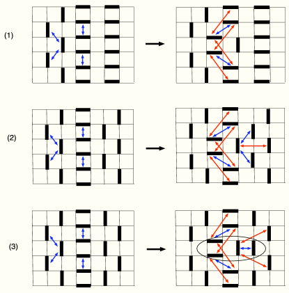
Figure 16: (Color online) The three types of intermediate states obtained by acting once with the perturbation 5 on the domain wall states. The blue/dark gray (red/light gray) arrows denote attractive (repulsive) interactions that are present in the initial (left) or excited (right) state but not both. The circled cluster of the excited state of (3) is another such interaction. (1) is a staggered line next to a columnar region of greater than unit width. (2) and (3) are staggered lines separated by one columnar strip from another staggered line of the same and opposite orientation respectively. Notice that relative to the excited state of (1), the excited state of (2) has 2 additional attractive $a$ bonds and 2 additional repulsive $c$ bonds. Similarly, excited state (3) has 1 additional attractive $b$ bond, 2 additional repulsive $d$ bonds, and a repulsive $p$ interaction. Since $c,d\geq a,b$, cases (2) and (3) involve higher energy intermediate states than (1).

The resonance energy of a particular staggered line depends on how the dimers next to the line are arranged. Fig. 16 shows the three possibilities that give denominators that may enter Eq. 6: The staggered line may be of type (1) next to a columnar region of greater than unit width (Fig. 16-1), or separated by one columnar strip from another staggered line of type (2), having the same orientation (Fig. 16-2) or type (3), having opposite (Fig. 16-3) orientation. From the figure, we see that cases (2) and (3) involve higher energy intermediate states than case (1) but allow for a denser packing of lines.

If $p$ is sufficiently large, states with type (3) lines will be disfavored as ground states. Ignoring such states, we update Eq. 4 to include second order corrections. For convenience, we set $c=a$ which removes the distinction between cases (1) and (2),

$$E(N_{s}) = -b\frac{N_{y}N_{x}}{2}+(b-a-\frac{t^{2}}{4d+2b})N_{y}N_{s}$$

We may use this to update the ground state phase diagram. If $b>a+\frac{t^{2}}{4d+2b}$, the system is optimized when $N_{s}=0$, which is the columnar phase. If $b<a+\frac{t^{2}}{4d+2b}$, the best domain wall state is the one with maximal staggering but without case (3) lines. This corresponds to the [11] state (Fig. 9a) in which every staggered strip has the same orientation. As $a-b$ is further increased, the herringbone state will eventually be favored. The boundary between the [11] and herringbone state may be determined by comparing energies. The energy of the [11] state is:

$$E_{[11]}=(-b-a-\frac{t^{2}}{4d+2b})\frac{N_{x}N_{y}}{4}+O(t^{4})$$ (8)

while the herringbone state has energy $E_{h}=-a\frac{N_{x}N_{y}}{2}$. From this, it follows that the [11] state will be favored when:

$$a-\frac{t^{2}}{4d+2b}<b<a+\frac{t^{2}}{4d+2b}$$ (9)

while the herringbone state will occur when $b<a-\frac{t^{2}}{4d+2b}$.

Therefore, up to corrections of order $t^{4}$, the system has the phase diagram shown in Fig. 10. Because the coefficient of $N_{s}$ in Eq. LABEL:eq:energy2 is zero on the [11]-columnar boundary, we have that the [11] state, columnar state, and any domain wall state with intermediate tilt (that contains only lines of type (1) and (2)) are degenerate on the boundary. In contrast, on the [11]-herringbone boundary, only the two states are degenerate.

In Appendix A, the more general case, where $c>a$, is discussed and the resulting phase diagram is shown in Fig. 17. An additional phase is stabilized in a region of width $\sim(c-a)t^{2}$ (assuming $|c-a|$ is finite) between the [11] and columnar states. In this new phase, labelled $A_{2}$, any state where adjacent staggered lines are separated by two columns, including the [12] state (Fig. 9b), is a ground state. These are the states which maximize the number of type (1) staggered lines (Fig. 16-1). On the [11]-$A_{2}$ boundary, intermediate states where adjacent staggered lines are separated by one or two columns (and where there are no type (3) lines) are degenerate. On the $A_{2}$-columnar boundary, states where adjacent staggered lines are separated by at least two columns are degenerate.

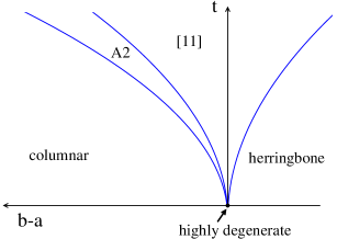
Figure 17: (Color online) Second order phase diagram when $c>a$. The [11] phase has width $\sim t^{2}$ and the $A_{2}$ phase has width $\sim(c-a)t^{2}$. On the [11]-$A_{2}$ and the $A_{2}$-columnar boundaries, intermediate domain wall states are degenerate as described in the text.

Fig. 17 may be understood intuitively by noting that at $a=b$ and $t=0$, a staggered strip has the same energy as a columnar strip. The resonance terms lower the effective energy of a staggered strip and since the [11] state involves the most staggered strips, its energy will be lowered the most. As $b$ increases to the point where the degeneracy between columnar strips and type (2) lines is restored, the system will prefer to maximize the number of type (1) lines, which are individually more stable but loosely packed. This is the transition to the $A_{2}$ phase. As $b$ is increased further, the degeneracy between columnar strips and type (1) lines is restored and there is a transition to the columnar state. Note that if $|c-a|$ is very large, [11]-$A_{2}$ boundary can occur in the $a>b$ region.

Before proceeding with the calculation, we clarify two points of potential confusion. First, when we say the “[11] state is stabilized” over part of the phase diagram, what we precisely mean is that the ground state wavefunction is a superposition of dimer coverings that has relatively large overlap with the literal [11] state of Fig. 9a and much smaller overlaps (of order $t^{2}$) with the excited states obtained by acting on the [11] state once with the perturbation 5 (Fig. 8). We use the notation [11] to denote both the perturbed wavefunction, which is an eigenstate of the perturbed Hamiltonian and the literal [11] state, which is an eigenstate of the unperturbed Hamiltonian. Second, the phase boundaries are based on a competition between a resonance term, which is a quantum version of “entropy”, and part of the zeroeth order piece which, continuing the classical analogy, is like an internal energy. This does not contradict the spirit of perturbation theory because the full zeroeth order term, $-b\frac{N_{y}N_{x}}{2}+(b-a)N_{y}N_{s}$, is always larger than the second order correction.

A similar phase diagram will occur (though at fourth order in perturbation theory) if we use the two-dimer move of Rokhsar-Kivelson. However, the bookkeeping will be more complicated because resonances will be able to originate in the interior of the columnar regions instead of just at that the columnar-staggered boundaries. This may be compensated by tuning $b$, which will merely move the boundaries, or by adding appropriate (local) repulsive terms to the parent Hamiltonian.

V.2.2 Fourth order

We concentrate on Fig. 17 as it is more generic than the fine-tuned $c=a$ case of Fig. 10. In either case, we expect the degeneracies on the phase boundaries to be partially lifted by considering higher orders in perturbation theory. In this section, we focus on the $A_{2}$-columnar boundary, where adjacent lines are separated by at least two columnar strips.

We return to the perturbation series for the energy (Eq. 6), this time keeping terms up to fourth order in the small parameter.

$$E_{n} = \epsilon_{n}-t^{2}\sum_{m}^{\prime}\frac{V_{nm}V_{mn}}{\epsilon_{m}-\epsilon_{n}}$$ (10)

$$- t^{4}\Bigl{[}\sum_{ml}^{\prime}\frac{V_{nm}V_{ml}V_{lk}V_{kn}}{(\epsilon_{m}-\epsilon_{n})(\epsilon_{l}-\epsilon_{n})(\epsilon_{k}-\epsilon_{n})}$$

$$- \sum_{ml}^{\prime}\frac{V_{nm}V_{mn}V_{nl}V_{ln}}{(\epsilon_{m}-\epsilon_{n})^{2}(\epsilon_{l}-\epsilon_{n})}\Bigr{]}+O(t^{6})$$

As usual, the primes denote that the sum is over all states except $|n\rangle$. The two fourth order terms correspond, in conventional Rayleigh-Schrodinger perturbation theory, to the corrections to the energy expectation value $\langle\psi|H|\psi\rangle$ and wavefunction normalization $\langle\psi|\psi\rangle$. We will refer to the corresponding terms as “energy” and “wavefunction” terms. As in the second order case, we may view the terms in the fourth order sums as virtual resonances connecting the initial state to itself via a series of high energy intermediate states. For this reason, we will refer to the summands as (fourth-order) “resonances”.

Most terms in the double sum in Eq. 10 correspond to resonances between disconnected clusters (Fig. 18). Referring to the figure, we use the term “disconnected” to indicate that there are no interaction terms connecting the dimers of clusters 1 and 2. While the number of such resonances scales as the square of the system size, the contributions from the energy and wavefunction terms in Eq. 10 precisely cancel for these disconnected clusters. The details of this cancellation are discussed in Appendix B.

The remaining fourth order resonances are extensive in number and may be grouped into three categories. In the first category, shown in Fig. 19, are resonances associated with a single staggered line and the number of such resonances in the system is proportional to the number of lines. We refer to these resonances as “self-energy corrections”.

In the second category, shown in Fig. 20, there are resonances that contribute to the effective interactions between adjacent lines. These resonances occur only in states where lines are separated by two or fewer columnar strips. Because we are interested in the $A_{2}$-columnar boundary, the only processes to consider are the ones shown in the figure. The purpose of terms $p$ and $q$ in Eq. 3 is to control the processes in Figs. 20a and b respectively. The net contribution of these resonances involve both energy and wavefunction terms. For example, the contribution of Fig. 20b to the energy is:

$$e=\frac{2t^{4}}{2(4d+2b)^{3}}\Bigl{[}1-\frac{1}{1+\frac{2q-a}{2(4d+2b)}}\Bigr{]}$$ (11)

and likewise for Fig. 20a (replace $2q-a$ with $2p-b$). If $q>a/2$, the net contribution of this resonance is repulsive.

The third type of resonance is the long resonance, shown in Fig. 21. These resonances occur in the energy term of Eq. 10 but do not have corresponding pieces in the wavefunction term. Therefore, these resonances will always lower the energy though, as the figure indicates, the precise amount depends on the way the lines are spaced.

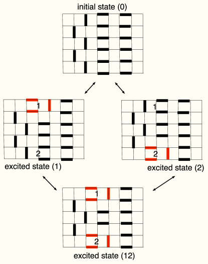
Figure 18: (Color online) Most of the fourth order terms in Eq. 10 involve “disconnected” clusters of dimers. In this figure, the perturbation connects the initial state (0) to excited states, labelled (1) and (2), depending on whether cluster 1 or 2 has been flipped. Acting again with the perturbation connects to an excited state, labeled (12), where both of these clusters are flipped. Acting two more times with the perturbation brings us back to the initial state (0) via either of excited states (1) or (2). Such terms are called disconnected because there are no interactions (in Eq. 3) between the dimers of clusters 1 and 2. The figure depicts a particular resonance from the energy term in Eq. 10. There is an analogous contribution from the wavefunction term which is a product of the second order processes $(0)\rightarrow(1)\rightarrow(0)$ and $(0)\rightarrow(2)\rightarrow(0)$. While the number of such disconnected terms scales as $N^{2}$, where $N=L_{x}L_{y}$ is the system size, these resonances do not contribute to the energy because the contributions from the energy and wavefunction terms exactly cancel.

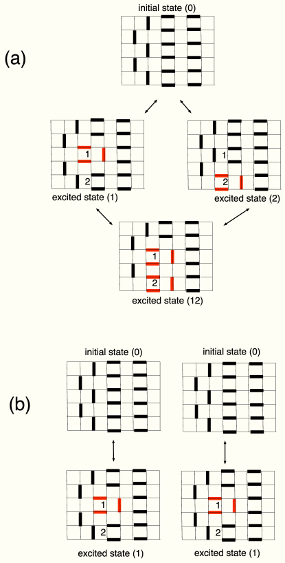
Figure 19: (Color online) These are examples of fourth order self-energy resonances. Each resonance is confined to a single line and the number of resonances in the system is proportional to the number of lines. In resonances such as (a), there are interactions connecting dimers of two flipped clusters on the same line. Terms such as (b) arise from the wavefunction term in Eq. 10 but have no analogous processes in the energy term to cancel against.

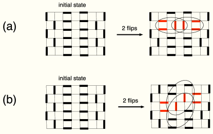
Figure 20: (Color online) These are examples of fourth order resonances which are effective interactions between lines. At fourth order, such interactions are possible only when lines are separated by two or fewer columns. On the $A_{2}$-columnar boundary, resonances (a) and (b) are the only processes to consider. These involve terms $p$ and $q$ in the Hamiltonian, as indicated by the circles.

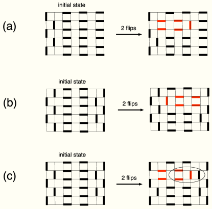
Figure 21: (Color online) These are the long fourth order resonances which occur in states where lines are separated by two or more columnar strips. These processes are always stabilizing though the amount depends on the environment of the line as in the second order (see Fig. 16). The resonance in (a) is strongest because it involves the lowest energy intermediate state but (b) and (c) allow for a denser packing of lines. Resonance (c) is especially suppressed due to term $p$ in Eq. 3.

An immediate implication of these resonances is the lifting of the degeneracy of the $A_{2}$ phase. All of these states have the same number of lines so will receive the same self-energy contribution (Fig. 19). If we choose $p,q$ large compared to $a,b,c$ and $d$, then the repulsive contribution from the interaction resonances (Fig. 20) is essentially determined by the wavefunction term, which is the same for all of the $A_{2}$ states. The degeneracy is broken by the long resonances because in the [12] state, only Fig. 21b processes occur while in the other $A_{2}$ states, some of the resonances are the suppressed Fig. 21c variety. Therefore, what was seen as merely an $A_{2}$ phase at second order is revealed, on closer inspection, as a [12] phase.

To investigate the degeneracy of what we now recognize as the [12]-columnar boundary, it is useful to update Eq. LABEL:eq:energy2 to include fourth order corrections:

$$E = -b\frac{N_{y}N_{x}}{2}+(b-a-\frac{t^{2}}{4d+2b}+\alpha t^{4})N_{y}N_{s}$$ (12)

$$- \beta t^{4}N_{y}N_{sa}-\gamma t^{4}N_{sb}+O(t^{6})$$

where $N_{s}$ is the total number of staggered lines and $N_{sa(b)}$ is the number of staggered lines having the environment of Fig. 21a(b). We ignore states with arrangements like Fig. 21c since they are disfavored as ground states. $\alpha$ is a constant, which may be calculated but whose value is unimportant, containing the contribution of fourth order self energy terms. $\beta=\frac{1}{(4d+2b)^{2}(2(4d+2b)+4(d-a))}>0$ is the contribution of the most favorable long fourth order resonances (Fig. 21a) whose number is proportional to $N_{sa}$. $\gamma=\frac{1}{(4d+2b)^{2}(2(4d+2b)+4(d-a)+2(c-a))}-2e$ ($e$ given by Eq. 11) is proportional to $N_{sb}$ and includes the contributions of Figs. 20b and 21b. Note that $\gamma<\beta$ and the sign of $\gamma$ is determined by the size of $q$. For convenience, we assume $q$ large enough that $\gamma<0$.

We may use Eq. 12 to correct the phase diagram. Similar to the second order case, as $b$ is increased, the extra stability of the staggered strips in the [12] state becomes eventually balanced by the zeroeth order energy of the columnar strips. When this occurs, the system will prefer a state with fewer lines that are individually more stable. In particular, the states we may label $A_{3}$, where adjacent lines are separated by three columns, maximize the number of favorable long resonances (Fig. 21a) without incurring any of the repulsive fourth order penalties (i. e. the analog of Fig. 20 would be a disconnected resonance). In the next section, higher order perturbation theory will show that this $A_{3}$ phase is actually a [13] phase (Fig. 9c) so we begin using the [13] label immediately. As $b$ is increased further, the system will enter the columnar state.

The result is the phase diagram in Fig. 22. The phase boundaries are determined by comparing energies. Ignoring corrections of order $t^{6}$, we have the following:

$$E_{[12]}=-b\frac{N_{y}N_{x}}{2}+(b-a-\frac{t^{2}}{4d+2b}+\alpha t^{4}-\gamma t^{4})\frac{N_{y}N_{x}}{6}$$

(13)

$$E_{[13]}=-b\frac{N_{y}N_{x}}{2}+(b-a-\frac{t^{2}}{4d+2b}+\alpha t^{4}-\beta t^{4})\frac{N_{y}N_{x}}{8}$$

(14)

$$E_{col}=-b\frac{N_{y}N_{x}}{2}$$ (15)

Comparing these expressions, we obtain the updated phase diagram shown in Fig. 22. The [12] state is favored when:

$$b<a+\frac{t^{2}}{4d+2b}-\alpha t^{4}-(4|\gamma|+3\beta)t^{4}$$ (16)

The [13] is favored when:

$$a + \frac{t^{2}}{4d+2b}-\alpha t^{4}-(4|\gamma|+3\beta)t^{4}<b$$

$$< a+\frac{t^{2}}{4d+2b}-\alpha t^{4}+\beta t^{4}$$

The columnar state is favored when:

$$b>a+\frac{t^{2}}{4d+2b}-\alpha t^{4}+\beta t^{4}$$ (18)

On the [12]-[13] boundary, there is a degeneracy between intermediate states where adjacent lines are separated by either two or three columnar strips. On the [13]-columnar boundary, there is a degeneracy between states where adjacent staggered lines are separated by at least two columns.

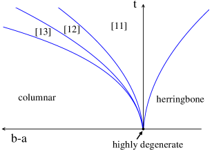
Figure 22: (Color online) Fourth order phase diagram. The new [13] state has width $\sim t^{4}$.

V.2.3 Higher orders and fine structure

The picture of Fig. 22 will be further refined by considering sixth order resonances and new phases will appear near the phase boundaries, in regions of width $~{}\sim t^{6}$, which is why they were missed at fourth order. The most immediate consequence will be the lifting of the degeneracy of the $A_{3}$ states in favor of the state [13]. The latter state, in comparison with the other $A_{3}$ states, is both stabilized maximally by the sixth order analog of Fig. 21 and, if we choose $p>q$, destabilized minimally by the sixth order analog of Fig. 20. The [13]-columnar phase boundary will open to reveal the [14] phase (Fig. 9d)foo (b), in which the number of favorable long resonances, the sixth order analogs of Fig. 21a, is maximized and there are no repulsive contributions ( i. e. the sixth order analogs of Fig. 20 will be disconnected terms if the lines are more than three columnar strips apart).

The argument may be applied iteratively at higher orders in perturbation theory. At 2n-th order, we may ask whether the [1n]-columnar boundary will open to reveal a new phase. The transition to less tilted states will be again be driven by processes that connect adjacent lines (Fig. 23). In the competitive states, adjacent lines are separated by at least n columnar strips so 2n-th order resonances connecting the lines must be “straight”. This means that the complicated high order processes, including “snake-like” fluctuations that break the staggered lines, will simply change the self-energy of a staggered line and do not have any effect on the transition. The [1n] phase will be destabilized by the process in Fig. 23b which will overwhelm the stabilizing effect of Fig. 23a due to combinatorics. However, these repulsive processes will not contribute when the lines are separated by more than n columnar strips. Therefore, the [1,n+1] phase, which maximizes the number of the long 2n-th order resonances (Fig. 23c), will be stabilized in a region of width $~{}\sim t^{2n}$ between the [1n] and columnar phases. Therefore, we obtain the phase diagram of Fig. 13.

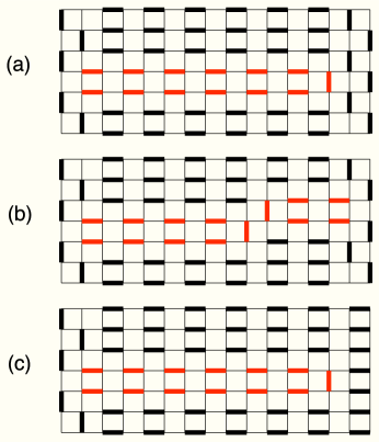
Figure 23: (Color online) These are the 12-th order resonances which drive the transition between the [16] and [17] states. Process (a) selects the [16] state from the others in the $A_{6}$ manifold, which were stabilized equally at 10th order. Process (b) destabilizes the [16] state near its columnar boundary in favor of the [17] state, which maximizes the number of most favorable resonances (c).

This shows that states with arbitrarily long periods are stabilized without long range interactions or fine tuning (other than the requirements of perturbation theory). The situation will be similar if we were to use the two-dimer Rokhsar-Kivelson resonance. In this case, there will be contributions from resonances occurring only in the columnar regions, which were “inert” in our calculation. These processes will amount to self-energy corrections that just renormalize columnar energy scale $b$. Also, additional local terms (i.e. other than $p$ and $q$) may be required to realize the very high-order states because adjacent lines will be able to interact via intermediate states other than the ones shown in Fig. 20. While we have not worked out the exact details of this case, we note that there are a finite number of such intermediates states so only a finite number of local terms will be required. In particular, we will not have to add longer terms at each order in perturbation theory.

So far, we have concentrated on the boundary with the columnar phase but we may also ask whether a similar lifting may occur on the other phase boundaries. We consider the [11]-[12] boundary. Both of these phases are stabilized at second order and occupy regions of width $~{}\sim t^{2}$ in the phase diagram (assuming $|c-a|\gg t^{2}$). On their boundary, all states where staggered lines are separated by either one or two columnar strips are degenerate to second order. We investigate the effect of fourth order resonances on this boundary.

We need to consider not only the resonances presented in section V.2.2 but also new fourth order processes which become available once we consider staggered lines that are one column apart. These are shown in Figs. 24 and 25. The resonances in section V.2.2 will stabilize (or destabilize – the sign is not important) each boundary state by an amount proportional to the number of its “[12] regions”, i. e. columnar regions that are two columns wide and have staggered lines on their boundary, while the resonances in Fig. 24 will contribute an amount proportional to the number of “[11] regions”, i. e. columnar regions that are one column wide. If these were the only available processes, the [11]-[12] boundary would be shifted by $\sim t^{4}$ but the degeneracy on the boundary would remain.

The possibility of a new phase is determined by the resonances in Fig. 25. Both of these resonances have an overall stabilizing effect (the contributions to the energy are negative) and depend on whether a [11] region is adjacent to another [11] region (Fig. 25a) or a [12] region (Fig. 25b). Because $c>a$, resonance (b) is stronger than (a), since its intermediate state has lower energy, but requires a lower density of staggered lines. If the net contribution of resonance (a) wins, then the degeneracy would be lifted in favor of the [11] state and the [11]-[12] boundary would be shifted again, but the degeneracy will only be between the two states. However, if $c$ is made sufficiently largefoo (c), the contribution of resonance (a) tends to zero while (b) approaches a constant because the intermediate state can occur without involving $c$ bonds (i. e. the fourth order process where the left cluster is flipped first and last). Therefore, there will be a new phase where resonance (b) is maximized. This state is the [11-12] state where the label refers to the repeating unit “one staggered strip followed by one columnar strip followed by one staggered strip followed by two columnar strips”.

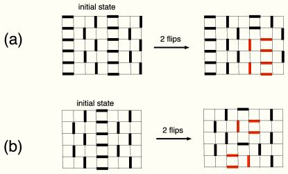
Figure 24: (Color online) These are fourth order processes available between two staggered lines separated by a single columnar strip.

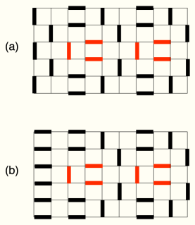
Figure 25: (Color online) These are fourth order processes which can occur if a [11] region is next to (a) another [11] region or (b) a [12] region. Both of these resonances contribute to the energy with a negative sign because the intermediate state involves two fewer repulsive $c$ bonds than if the flipped clusters were farther apart.

Continuing the line of thought, we may ask whether the [11-12]-[12] boundary will open at higher orders. Sixth order resonances will shift the boundary but there are no processes which break the degeneracy. However, at eighth order, there is a resonance which will favor a [11-(12)²] phase (Fig. 26).

We can, in principle, investigate whether the [11-(12)ⁿ] phases continue to appear when n is large and also whether the new boundaries themselves open to reveal even finer details. The same arguments will hold for all of the other boundaries in the [1n] sequence. While the structure of our Hamiltonian allowed us to be definite regarding the [1n] sequence, it is more difficult to draw conclusions about the fine structure at high orders in perturbation theory because increasingly complicated resonances need to be accounted for. Most of these resonances will stabilize the unit cells of the states on either side of the boundary so the net effect will be to move the boundary. The more important terms, with respect to whether boundaries will open, are resonances associated with interfaces between regions with one or another unit cell. Even these terms can become complicated at very high orders in perturbation theory. However, our arguments suggest that arbitrarily complicated phases can, in principle, be stabilized by going to an appropriate range in parameter space and/or adding additional local interactions. Therefore, the most generic situation is an incomplete devil’s staircase, as sketched in Fig. 14.

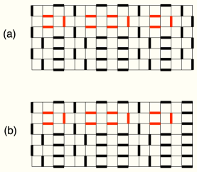
Figure 26: (Color online) These are eighth order processes which can lead to a new phase between the [11-12] and [12] phases. Resonance (a) stabilizes the [11-12] phase while (b) stabilizes the [11-(12)²] phase. In the limit where $c$ is large, resonance (b) is preferable. The easiest way to see this is by setting $c=\infty$. Then the energy term of resonance (a) and all of the wavefunction terms in resonances (a) and (b) will give zero because the intermediate states can not form without creating $c$ bonds. However, the intermediate state in resonance (b) does not involve $c$ bonds and can be obtained without creating $c$ bonds (i. e. in an eighth order process where the first and last two actions involve flipping the cluster on the right and the first cluster in the middle). Therefore, the energy term of resonance (b) will give a stabilizing contribution.

V.3 Order of the transitions between the $[1n]$ phases

The boundaries between different modulated states are generically first-order. Intuitively, this is not surprising because of the topological property that “protects” the states, namely that even with an infinite number of local dimer moves, it is impossible to go from one state to the other since the states are in different topological sectors. Therefore, we would not expect a transition to be driven by a growing correlation length.

Formally, the way we use to determine the order of the transitions that emerge in the system, is by calculating the first derivative of the ground-state energy on either side of the phase boundaries that we found.Sachdev (1999) For example, we will treat explicitly the case of the transition between $[12]\rightarrow[13]$, even though the same line of argument applies to the other boundaries as well. The energies of the two states near the phase boundary, are given by Eq. 13, Eq. 14 and the phase boundary is given by the following condition(as can be seen in Eq. 16):

$$b=a+\frac{t^{2}}{4d+2b}-\alpha t^{4}-(4|\gamma|+3\beta)t^{4}$$ (19)

Let’s consider the case where we approach the boundary from the $[12]$ side varying the variable $t$ but keeping $a,b$ constant. In the phase diagram Fig. 13, we ’move’ vertically down. The reason for choosing this direction is just clarity. Let’s call the point of the phase boundary where our path crosses, $A$, and the critical value of t, $t_{c}$ (coming from the solution of Eq. 19 for fixed values of $a,b,d$).

The energies of the two states at the phase boundary are exactly equal. Their derivatives are:

$$\frac{\partial E_{[12]}}{\partial t}\Bigg{|}_{A^{+},t_{c}} = -(\frac{2t_{c}}{4d+2b}-4\alpha t_{c}^{3}-4|\gamma|t_{c}^{3})\frac{N_{y}N_{x}}{6}$$ (20)

$$+O(t_{c}^{5})$$

$$\frac{\partial E_{[13]}}{\partial t}\Bigg{|}_{A^{-},t_{c}} = -(\frac{2t_{c}}{4d+2b}-4\alpha t_{c}^{3}+4\beta t_{c}^{3})\frac{N_{y}N_{x}}{8}$$ (21)

$$+O(t_{c}^{5})$$

By Eqs. 19, 20 and 21, we have:

$$\frac{\partial E_{[12]}}{\partial t}\Bigg{|}_{A^{+},t_{c}}-\frac{\partial E_{[13]}}{\partial t}\Bigg{|}_{A^{-},t_{c}}=$$

$$\underbrace{\left(\frac{t_{c}}{2(4d+2b)}-\frac{b-a}{t_{c}}\right)}_{<0{\rm\;to\;order}\;O(t^{2})}\frac{N_{y}N_{x}}{6}+O(t_{c}^{5})$$ (22)

The derivatives are not equal along the phase boundary so the transition is discontinuous (first-order). It is clear that all the phase transitions we found will also be discontinuous because the above discontinuity comes exactly from the contributions leading to the phase boundary’s presence.

VI Connections with frustrated Ising models

A natural question to ask is whether the staircase presented above has any connection to the staircase of the 3D ANNNI model or the quantum analogs discussed in Ref. Harris et al., 1995a. One of the main differences of the present work is the non-perturbative inclusion of frustration by considering hard-core dimers as the fundamental degrees of freedom. In this sense, the present staircase differs from previous work similarly to how the fully frustrated Ising model differs from the conventional Ising model. It is instructive to consider the mapping between dimer coverings and configurations of the fully frustrated Ising model on the square lattice (FFSI) in more detail.

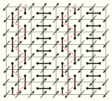
Figure 27: (Color online) One of the four possible $[11]$ configuration in terms of Ising spins on the fully frustrated square lattice. The hard-core dimer constraint corresponds to the requirement that the FFSI ground state has one “unsatisfied” bond per plaquette. The columnar-dimer regions correspond to ferromagnetic-Ising domains. The staggered-dimer strips correspond to the Ising domain walls, depicted by the red-colored (dashed) curved lines, which separate ferromagnetic domains of different orientation. Clearly, in the other equivalent configurations, even though they share the same principle of domain-wall competition, the separated regions are not ferromagnetic but one of several metamagnetic choices Liebmann (1984).

The FFSI model can be described in terms of Ising degrees of freedom living on the square lattice. The main difference with the usual ferromagnetic Ising model is the following: Even though in the x-direction, all the bonds are ferromagnetic, in the y-direction there are alternating ferromagnetic (antiferromagnetic) lines where ferromagnetic (antiferromagnetic) vertical bonds live (we consider that the absolute values of the couplings of all bonds are equal). In this way, the product of bonds on a single plaquette is always $-1$ (three ferromagnetic bonds per plaquette) and therefore the ground-state of the system cannot be just the ferromagnetic one. In fact, by mapping each ”unsatisfied” bond to a dimer living on the dual sublattice, we find that each of the degenerate ground-state configuration maps to a hard-core dimer configuration on the square lattice (see Fig.27) Liebmann (1984).

A typical [1n] configuration in the dimer language we used, as clearly depicted in Fig. 27 for one of the four equivalent dimer structures, under $\pi/2$ rotations and sublattice shifts, can be seen in the FFSI picture as ferromagnetic stripes of length $4n$ in the one direction and infinite in the other, separated by antiferromagnetic domain walls. In this way, these ordered states clearly resemble the modulated phases of the ANNNI model in two dimensions. The other three equivalent dimer structures map again to periodic domains in the Ising model, but with more complicated metamagnetic structure. The reason for this seemingly large complexity has to do with the fact that the possible equilibrium configurations have to satisfy the FFSI constraint.

As far as the interactions are concerned, we have the following correspondences: The three-dimer resonance term we used in our construction corresponds to a two neighboring-spins flip process which should, however, respect the FFSI constraint. We should note that the usual single-plaquette resonance move maps to the single-spin flip which is the same as the Ising transverse field usually considered. The $a$ and $b$-terms correspond to domain-wall energies in the FFSI. Both of them have an one-to-one mapping to three-spin interactions but these interactions are also anisotropic (they depend on the distribution of the Ising bonds which we described). The additional interactions that we added to the system, so that to extensively study it, correspond clearly to complicated multi-spin interactions.

VII Discussion

There are reasons to be optimistic that these ideas apply more generally. For example, as mentioned earlier, we expect that with suitable modification of Eq. 3, a similar phase diagram may be obtained for a wide variety of off-diagonal resonance terms, including the familiar two-dimer resonance of Rokhsar-Kivelson. This is because the perturbation theory is structured so that at any order, most of the nontrivial resonances amount to self-energy corrections and the resonances driving the transitions are comparatively simpler. The three-dimer resonance of Eq. 2 is analytically convenient as its action is confined to the domain wall boundaries. The two-dimer resonance would involve more complicated bookkeeping since we also need to account for internal fluctuations of the columnar regions.

Another reason to expect these ideas to hold more generally is the qualitative similarity of this approach to the field theoretic arguments in Refs. Vishwanath et al., 2004 and Fradkin et al., 2004. In those studies, the following action, in the notation of Ref. Fradkin et al., 2004, was used to describe the tilting transition in the Rokhsar-Kivelson quantum dimer model on the honeycomb lattice (the square lattice is similar but with some added subtleties – see Ref. Fradkin et al., 2004):

$$S = \frac{1}{2}(\partial_{\tau}h)^{2}+\frac{1}{2}\rho_{2}(\nabla h)^{2}+\frac{1}{2}\rho_{4}(\nabla^{2}h)^{2}$$ (23)

$$+ g_{3}(\partial_{x}h)(\frac{1}{2}\partial_{x}h-\frac{\sqrt{3}}{2}\partial_{y}h)(\frac{1}{2}\partial_{x}h+\frac{\sqrt{3}}{2}\partial_{y}h)$$

$$+ g_{4}|\nabla h\cdot\nabla h|^{2}+\ldots$$

where “$\ldots$” includes terms that are irrelevant to the present discussion (though maybe not strictly “irrelevant” in the RG sense). In this expression, $h$ is a coarse grained version of the height field (Fig. 5) and the first line of Eq. 23 describes the tilting transition at the RK pointact , which corresponds to $\rho_{2}=g_{3}=g_{4}=0$. If $g_{3}<0$, the system favors tilted states and is similar to our parameter $a-b$. However, $g_{4}$ prevents the tilt from taking its maximal value and in this sense, is similar to our terms $c$ and $d$. The existence of the devil’s staircase in Ref. Fradkin et al., 2004 was established by tuning $g_{3}$ and $g_{4}$ so as to stabilize an intermediate tilt and then to study the fluctuations about this state. The staircase arose from a competition between these quantum fluctuations, analogous to our term $t$, and lattice interactions, (roughly) analogous to our terms $c$, $d$, $p$, and $q$.

Another sense in which our calculation is similar to Ref. Fradkin et al., 2004 may be seen by heuristically considering the effect of doping the model. In particular, consider replacing one of the dimers in a staggered strip with two monomers. If we then separate the monomers in the direction parallel to the stripe, a string of columnar bonds will be created. If the staggered and columnar bonds were degenerate, then this would cost no energy in addition to the cost of creating the monomers in the first place so the monomers would be deconfined. However, in the [1n] phase, the staggered bonds are slightly favored so the energy cost $E$ of separating the monomers by a distance $R$ would be $E\sim Rt^{2n}$. Hence, the commensurate phases seen in our model are confining with a confinement length that becomes arbitrarily large for the high-order structures that appear very close to the columnar phase boundary. This is qualitatively similar to the “Cantor deconfinement” scenario proposed in Ref. Fradkin et al., 2004.

However, there are ways in which our calculation is qualitatively different from the above. Our calculation takes place in the limit of “strong-coupling” where $t$ is small compared with other terms but influences the phase diagram nonetheless because the stronger terms are competing. In contrast, the RK point of a quantum dimer model, by definition, occurs in a regime of parameter space where quantum fluctuations are comparable in strength to the interactions. The field theoretic prediction requires $g_{3}$ and $g_{4}$ being nonzero so does not literally apply at the RK point either but, by self-consistency, should apply somewhat “near” it. We may speculate that the tilted states being predicted by the field theory are large $t$ continuations of states that emerge in the strong coupling limit far from the RK point. However, we reemphasize that our calculation is reliable only in the limit of small $t$ and we can not be certain which (if any) of our striped phases survive at larger $t$. Another issue is that the phase diagram near the RK point depends strongly on the lattice geometry and the prediction of a devil’s staircase in Ref. Fradkin et al., 2004 is for bipartite lattices. In contrast, lattice symmetry does not play an obvious role in the present work and it is likely that these ideas can be made to apply on more general lattices.

It is also likely that this calculation can be made to work in the strong-coupling limits of other frustrated models, for example vertex modelsArdonne et al. (2004) and even in higher dimensions. For example, mappings similar to those discussed in Ref. Raman et al., 2005 may be used to construct an SU(2)-invariant spin model on a decorated lattice that displays the same phases. A more interesting direction would be to study the strong-coupling limits of more physical models, for example the Emery model of high $T_{c}$ superconductivityEmery (1987) which also shows an affinity for nematic ground statesKivelson et al. (2004). It would also be interesting to see whether nematicity is essential, i. e. whether other types of phase separation can occur in a purely local model through effective long range interactions that arise, as in the present calculation, from the interplay of kinetic energy and frustration.

Appendix A Details of the second order calculation

In this section, we explicitly work out the details of the second order calculation, including the effect of having $c>a$. We show that the second order phase diagram is qualitatively similar to the $c=a$ case presented in the main text, provided that $c$ is not too large (the precise condition is obtained below). Therefore, fine-tuning to $c=a$ is purely a matter of convenience.

With reference to Fig. 16, we may calculate the difference in energy between the excited and initial states for each case. The unperturbed energies $\epsilon_{i}^{in}$, $i\in\{1,2,3\}$, of the initial states in Fig. 16-1, 16-2, and 16-3 are given by Eq. 4 and are degenerate when $a=b$. To calculate the unperturbed energies, $\epsilon_{i}^{ex}$ of the excited states, we need to examine the interaction energies present in the excited states which are absent in the initial states and vice versa. These are shown in Fig. 16 by the red and blue arrows. Using the figure, we obtain:

$$\epsilon_{1}^{ex}-\epsilon_{1}^{in} = (4d-2a)-(-2a-2b)$$ (24)

$$= 4d+2b$$

$$\epsilon_{2}^{ex}-\epsilon_{2}^{in} = (4d+2c-2a-2a)-(-2a-2b)$$ (25)

$$= 4d+2b+2c-2a$$

$$\epsilon_{3}^{ex}-\epsilon_{3}^{in} = (6d+p-2a-b)-(-2a-2b)$$ (26)

$$= 6d+p+b$$

These are the three possible energy denominators which may enter Eq. 6. We may classify a staggered line based on the dimer arrangement to its immediate right, corresponding to cases (1), (2), and (3) in Fig. 16. Each staggered line contributes $-N_{y}\frac{t^{2}}{\epsilon_{i}^{ex}-\epsilon_{i}^{in}}$. The factor $N_{y}$ is because there are $\frac{N_{y}}{2}$ possible rightward resonances of each line and also $\frac{N_{y}}{2}$ leftward resonances of the line to its right, which enter with the same weight. Putting everything together, we can update Eq. 4:

$$E(N_{s1},N_{s2},N_{s3},N_{c}) = -b\frac{N_{y}N_{x}}{2}+(b-a)N_{y}N_{s}$$ (27)

$$- N_{y}N_{s1}\frac{t^{2}}{4d+2b}$$

$$- N_{y}N_{s2}\frac{t^{2}}{4d+2b+2c-2a}$$

$$- N_{y}N_{s3}\frac{t^{2}}{6d+p+b}$$

$$+ O(t^{4})$$

where $N_{si}$ is the number of staggered lines of type (i) and $N_{s}=N_{s1}+N_{s2}+N_{s3}$ is the total number of staggered lines. While the zeroeth order term depends only on the number of staggered lines, the $O(t^{2})$ piece depends on their distribution and relative orientations.

Eq. 27 shows that type (1) staggered lines will be stabilized more by the perturbation than type (2) lines. However, the zeroeth order term depends only on the total number of lines and type (2) lines permit a denser packing of lines. We temporarily ignore type (3) lines. Depending on $b-a$, the system will favor either the [11] state, the columnar state, or the states which maximize the number of type (1) lines, which (at second order) are analogous to the maximally staggered configurations in Fig. 7 except staggered lines are now separated by two columns. We denote the latter collection of states with the label $A_{2}$ (i. e. alternating states where staggered strips alternate with two columns of columnar dimers). To determine these boundaries, we first write down the energies of these three states to second order in $t$ using Eq. 27:

$$E_{[11]}=-b\frac{N_{y}N_{x}}{2}-\frac{N_{y}N_{x}}{2}(b-a-\frac{t^{2}}{4d+2b+2(c-a)})$$ (28)

$$E_{A_{2}}=-b\frac{N_{y}N_{x}}{2}-\frac{N_{y}N_{x}}{4}(b-a-\frac{t^{2}}{4d+2b})$$ (29)

$$E_{col}=-b\frac{N_{y}N_{x}}{2}$$ (30)

where we have used $N_{s}=\frac{N_{x}}{4}$ for the [11] state, $N_{s}=\frac{N_{x}}{6}$ for the $A_{2}$ states, and $N_{s}=0$ for the columnar state. Comparing these expressions, we obtain the following boundaries. The [11] state is favored when:

$$b<a+\frac{t^{2}}{4d+2b}-\frac{3t^{2}}{2(4d+2b)}(1-\frac{4d+2b}{4d+2b+2(c-a)})$$ (31)

The $A_{2}$ states are favored when:

$$a+\frac{t^{2}}{4d+2b}-\frac{3t^{2}}{2(4d+2b)}(1-\frac{4d+2b}{4d+2b+2(c-a)})<b$$

$$<a+\frac{t^{2}}{4d+2b}$$

and the columnar state is favored when:

$$b>a+\frac{t^{2}}{4d+2b}$$ (33)

If we require that $(c-a)$ is small compared to $2d+b$ (recall that $d\geq a$ by assumption), then we see that the region where the $A_{2}$ state is preferred is a small region within the phase boundary of Fig. 10. The width of this region tends to zero as $c\rightarrow a$. A cartoon of this case is given in Fig. 17. On the $A_{2}$-columnar boundary, the $A_{2}$ states are degenerate with the columnar state and any intermediate state where consecutive staggered lines are separated by at least two columns. Similarly, on the [11]-$A_{2}$ boundary, the [11] states are degenerate with the $A_{2}$ states and any intermediate states where staggered lines of different (same) orientation are separated by two (either one or two) columns.

The collection of $A_{2}$ states are degenerate to order $t^{2}$. As the degeneracy of the $A_{2}$ states will be partially lifted at fourth order in the perturbation theory, the $c>a$ case adds complexity without changing the phase diagram qualitatively. Therefore, purely for convenience, we assume $c=a$ throughout the main text.

As $c$ is made larger, the width of the $A_{2}$ region increases but when $c>d+a+\frac{p-b}{2}$, then according to Eq. 27, we need to consider type (3) lines. In this case, the tilted state will no longer be favored and, in fact, all of the steps of the staircase will lie in the zero winding number sector.

Appendix B Cancellation of disconnected resonances

We now demonstrate the cancellation of disconnected terms that appear at fourth order in the perturbation theory (Eq. 10). Because our Hamiltonian is local, there are linked cluster theorems which ensure that this cancellation occurs at any order in the perturbation theory so the contribution to the energy is always extensive as it should be.

Regarding the situation of Fig. 18, we may write down all fourth order terms involving the excited states which we have labelled 1 and 2. The energy numerator will contribute a number of terms, each having energy:

$$E = -t^{4}\frac{V_{nm}V_{ml}V_{lk}V_{kn}}{(\epsilon_{m}-\epsilon_{n})(\epsilon_{l}-\epsilon_{n})(\epsilon_{k}-\epsilon_{n})}$$ (34)

$$= \frac{-t^{4}}{(4d+2b)^{2}(2(4d+2b))}$$

which follows because the energy of the excited states (relative to the initial state) are $\epsilon_{1}-\epsilon_{0}=\epsilon_{2}-\epsilon_{0}=4d+2b$ and $\epsilon_{12}-\epsilon_{0}=2(4d+2b)$. That $\epsilon_{12}-\epsilon_{0}=2(\epsilon_{1}-\epsilon_{0})$ is precisely because clusters 1 and 2 are disconnected. This would not be the case if we had a long range interaction. From Fig. 18, we readily see that there will be four such terms since there are four ways to connect the initial state (0) to the excited state (12) and then back to itself. Therefore, the full potentially pathological contribution of the energy numerator is:

$$E_{num}=-4\frac{t^{4}}{(4d+2b)^{2}(2(4d+2b))}=-2\frac{t^{4}}{(4d+2b)^{3}}$$ (35)

It is evident that there are of order $N^{2}$ of these terms because the choice of clusters 1 and 2 were arbitrary. The energy denominator (wavefunction normalization) will contribute terms, each having energy:

$$E=t^{4}\frac{V_{nm}V_{mn}V_{nl}V_{ln}}{(\epsilon_{m}-\epsilon_{n})^{2}(\epsilon_{l}-\epsilon_{n})}=\frac{t^{4}}{(4d+2b)^{3}}$$ (36)

and only resonances from the initial state to excited states 1 and 2 are involved. Because the case where $m=l$ gives an extensive contribution to the energy, we will be concerned with the case where $m$ and $l$ in the above equation are different. There are two such terms because either $m$ or $l$ can correspond to excited state 1 and the other to state 2. Therefore, the full potentially pathological contribution of the energy denominator is:

$$E_{den}=2\frac{t^{4}}{(4d+2b)^{3}}$$ (37)

We see explicitly that the non-extensive contributions of $E_{num}$ and $E_{den}$ precisely cancel. Clearly this will be case for any choice of disconnected clusters 1 and 2 so we have shown that, to fourth order in the perturbation theory, the energy correction is extensive, as it physically should be.

References

- Anderson (1987) P. W. Anderson, Science 235, 1196 (1987).
- Kivelson et al. (1987) S. A. Kivelson, D. S. Rokhsar, and J. P. Sethna, Phys. Rev. B 35, R8865 (1987).
- Lee et al. (2006) P. A. Lee, N. Nagaosa, and X.-G. Wen, Rev. Mod. Phys. 78, 17 (2006).
- Senthil and Fisher (2000) T. Senthil and M. P. A. Fisher, Phys. Rev. B 62, 7850 (2000).
- Hermele et al. (2005) M. Hermele, T. Senthil, and M. P. A. Fisher, Phys. Rev. B 72, 104404 (2005).
- Mudry and Fradkin (1994) C. Mudry and E. Fradkin, Phys. Rev. B 49, 5200 (1994).
- Emery and Kivelson (1993) V. J. Emery and S. A. Kivelson, Physica C 209, 597 (1993).
- Emery et al. (1999) V. J. Emery, S. A. Kivelson, and J. M. Tranquada, Proc. Natl. Acad. Sci. USA 96, 8814 (1999).
- Kivelson et al. (1998) S. A. Kivelson, E. Fradkin, and V. J. Emery, Nature 393, 550 (1998).
- Kivelson and Fradkin (2006) S. A. Kivelson and E. Fradkin, How optimal inhomogeneity produces high temperature superconductivity, to appear in Treatise of High Temperature Superconductivity, edited by J. R. Schrieffer and J. Brooks, in press (Springer-Verlag, Berlin); cond-mat/0507459 (2006).
- Kivelson et al. (2003) S. A. Kivelson, I. P. Bindloss, E. Fradkin, V. Oganesyan, J. Tranquada, A. Kapitulnik, and C. Howald, Rev. Mod. Phys. 75, 1201 (2003).
- Mackenzie and Maeno (2003) A. P. Mackenzie and Y. Maeno, Rev. Mod. Phys. 75, 657 (2003).
- Coldea et al. (2001) R. Coldea, D. A. Tennant, A. M. Tsvelik, and Z. Tylczynski, Phys. Rev. Lett. 86, 1335 (2001).
- Shimizu et al. (2003) Y. Shimizu, K. Miyagawa, K. Kanoda, M. Maesato, and G. Saito, Phys. Rev. Lett. 91, 107001 (2003).
- Ramirez et al. (1999) A. P. Ramirez, A. Hayashi, R. J. Cava, R. Siddarthan, and B. S. Shastri, Nature 399, 333 (1999).
- Snyder et al. (2004) J. Snyder, B. G. Ueland, J. S. Slusky, H. Karunadasa, R. J. Cava, and P. Schiffer, Phys. Rev. B 69, 064414 (2004).
- Löw et al. (1994) U. Löw, V. J. Emery, K. Fabricius, and S. A. Kivelson, Phys. Rev. Lett. 72, 1918 (1994).
- Lorenzana et al. (2001) J. Lorenzana, C. Castellani, and C. DiCastro, Phys. Rev. B 64, 235127 (2001).
- Jamei et al. (2005) R. Jamei, S. Kivelson, and B. Spivak, Phys. Rev. Lett. 94, 056805 (2005).
- Ravenhall et al. (1983) D. G. Ravenhall, C. J. Pethick, and J. R. Wilson, Phys. Rev. Lett. 50, 2066 (1983).
- Lorenz et al. (1993) C. P. Lorenz, D. G. Ravenhall, and C. J. Pethick, Phys. Rev. Lett. 70, 379 (1993).
- Seul and Andelman (1995) M. Seul and D. Andelman, Science 267, 476 (1995).
- Rokhsar and Kivelson (1988) D. S. Rokhsar and S. A. Kivelson, Phys. Rev. Lett. 61, 2376 (1988).
- Fisher and Selke (1980) M. E. Fisher and W. Selke, Phys. Rev. Lett. 44, 1502 (1980).
- Bak (1982) P. Bak, Rep. Prog. Phys. 45, 587 (1982).
- Moessner et al. (2002) R. Moessner, S. L. Sondhi, and E. Fradkin, Phys. Rev. B 65, 024504 (2002).
- Ardonne et al. (2004) E. Ardonne, P. Fendley, and E. Fradkin, Ann. Phys. (N. Y.) 310, 493 (2004).
- Vishwanath et al. (2004) A. Vishwanath, L. Balents, and T. Senthil, Phys. Rev. B 69, 224416 (2004).
- Fradkin et al. (2004) E. Fradkin, D. A. Huse, R. Moessner, V. Oganesyan, and S. L. Sondhi, Phys. Rev. B 69, 224415 (2004).
- Moessner and Sondhi (2001) R. Moessner and S. L. Sondhi, Phys. Rev. Lett. 86, 1881 (2001).
- Kitaev (2006) A. Kitaev, Ann. Phys. (N. Y.) 321, 2 (2006).
- Hermele et al. (2004) M. Hermele, M. P. A. Fisher, and L. Balents, Phys. Rev. B 69, 064404 (2004).
- Balents et al. (2002) L. Balents, M. P. A. Fisher, and S. M. Girvin, Phys. Rev. B 65, 224412 (2002).
- Fujimoto (2005) S. Fujimoto, Phys. Rev. B 72, 024429 (2005).
- Raman et al. (2005) K. S. Raman, R. Moessner, and S. L. Sondhi, Phys. Rev. B 72, 064413 (2005).
- Damle and Senthil (2006) K. Damle and T. Senthil, Phys. Rev. Lett. 97, 067202 (2006).
- Isakov et al. (2006) S. V. Isakov, Y. B. Kim, and A. Paramekanti, Phys. Rev. Lett. 97, 207204 (2006).
- Sengupta et al. (2006) K. Sengupta, S. V. Isakov, and Y. B. Kim, Phys. Rev. B 73, 245103 (2006).
- Fradkin and Kivelson (1990) E. Fradkin and S. A. Kivelson, Mod. Phys. Lett. B 4, 225 (1990).
- Balents et al. (2005a) L. Balents, L. Bartosch, A. Burkov, S. Sachdev, and K. Sengupta, Phys. Rev. B 71, 144508 (2005a).
- Balents et al. (2005b) L. Balents, L. Bartosch, A. Burkov, S. Sachdev, and K. Sengupta, Phys. Rev. B 71, 144509 (2005b).
- Vojta and Sachdev (1999) M. Vojta and S. Sachdev, Phys. Rev. Lett. 83, 3916 (1999).
- Zaanen and Gunnarsson (1989) J. Zaanen and O. Gunnarsson, Phys. Rev. B. 40, R7391 (1989).
- Zhang and Henley (2003) N. G. Zhang and C. L. Henley, Phys. Rev. B. 68, 014506 (2003).
- Emery (1987) V. J. Emery, Phys. Rev. Lett. 58, 2794 (1987).
- Kivelson et al. (2004) S. A. Kivelson, E. Fradkin, and T. H. Geballe, Phys. Rev. B 69, 144505 (2004).
- Balents et al. (2004) L. Balents, L. Bartosch, A. Burkov, S. Sachdev, and K. Sengupta, in Physics of Strongly Correlated Electron Systems, YKIS2004 workshop (Yukawa Institute, Kyoto, Japan, 2004).
- Pokrovsky and Talapov (1978) V. I. Pokrovsky and A. L. Talapov, JETP 75, 1151 (1978).
- Bak and von Boehm (1980) P. Bak and J. von Boehm, Phys. Rev. B 21, 5297 (1980).
- (50) The incomplete devil’s staircas is seen in the ANNNI model in three and higher dimensions. The perturbation series in Ref. Fisher and Selke, 1980 does not converge for . Numerical studies of the 2D model, discussed in Ref. Bak, 1982, indicate a floating phase, i.e. the wavevector of the modulation varies smoothly as the parameters in the model are varied (as opposed to locking at certain commensurate values).
- Harris et al. (1995a) A. B. Harris, C. Micheletti, and J. M. Yeomans, Phys. Rev. Lett. 74, 3045 (1995a).
- Harris et al. (1995b) A. B. Harris, C. Micheletti, and J. M. Yeomans, Phys. Rev. B. 52, 6684 (1995b).
- Blöte and Hilhorst (1982) H. W. J. Blöte and H. J. Hilhorst, J. Phys. A 15, L631 (1982).
- Henley (1997) C. L. Henley, J. Stat. Phys. 89, 483 (1997).
- (55) This conjectured action is the simplest action that captures a number of the salient features of the RK point, including the leading decay of correlation functions (by appropriately choosing and making the correct operator identifications — see Ref. Fradkin et al., 2004) and the large degeneracy in tilt. However, a systematic derivation of this action as the continuum limit of the Rokhsar-Kivelson (or any other) microscopic dimer model does not currently exist.
- (56) The RK point has the additional feature that the degenerate wavefunctions have no local order. At the RK point, the lowest energy state in each topological sector is one of the (degenerate) ground states of the system. In a given sector, the ground state wavefunction is the equal amplitude superposition of dimer coverings in that sector. Such a wavefunction will generally give zero expectation value for any local operator (except for special cases like the staggered state (Fig. 5b) which is the only dimer covering in its sector).
- (57) Hamiltonians with special points of large degeneracy were also considered recently in: Z. Nussinov, C. D. Batista, B. Normand, and S. A. Trugman, cond-mat/0602528.
- foo (a) This means that the period of the repeating unit becomes infinite. This becomes the case, for example, close to the boundary with the columnar phase but may also occur between the other phases.
- (59) In particular, the existence of arbitrarily long periods does not require sending , or even that these terms be orders of magnitude larger than .
- foo (b) Although we will only “know” this at eighth order when the degeneracy of the states, where adjacent lines are always separated by four columnar strips, is lifted in favor the one with maximal tilt.
- foo (c) We should consider to be large in comparison to the scale of the perturbation series, which is the difference . However, as it is pointed out in Appendix A, cannot be too large or equivalently, any of the couplings should be larger than . It is worth remarking that the choice of the magnitude of does not require, clearly, any fine-tuning.
- Sachdev (1999) S. Sachdev, Quantum Phase Transitions (Cambridge University Press, Cambridge, 1999).
- Liebmann (1984) R. Liebmann, Statistical Mechanics of Periodic Frustrated Ising Systems (Springer-Verlag, Berlin, 1984).