The Stochastic Flow Rule:
A Multi-Scale Model for Granular Plasticity

Abstract

In spite of many attempts to model dense granular flow, there is still no general theory capable of describing different types of flows, such as gravity-driven drainage in silos and wall-driven shear flows in Couette cells. Here, we summarize our recent proposal of the Stochastic Flow Rule (SFR), which is able to describe these cases in good agreement with experiments, and we focus on testing the theory in more detail against brute-force simulations with the discrete-element method (DEM). The SFR is a general rate-independent constitutive law for plastic flow, based on diffusing “spots” of fluidization. In the case of quasi-2D granular materials, we assume limit-state stresses from Mohr-Coulomb plasticity and postulate that spots undergo biased random walks along slip-lines, driven by local stress imbalances. We compare analytical predictions of the SFR against DEM simulations for silos and Couette cells, carrying out several parametric studies in the latter case, and find good agreement.

1 Introduction

Even after centuries of study, dense granular flow remains an enigma for both physicists and engineers [12, 2]. For dilute, collisional granular media, the kinetic theory of dissipative gases has been quite successful at describing the mean flow statistics [7]. On the opposite side of the spectrum, where the material is solid-like and possesses a yield function, the stresses and (to a lesser extent) the dynamics can be adequately described by methods of modern soil mechanics [26, 33]. However, the intermediate regime where the flow is slow, steady, and dense, has resisted many theoretical attempts [3, 14].

We have recently proposed the Stochastic Flow Rule (SFR) for dense granular flows [14]. It is a rate-independent constitutive law for steady flow which we believe naturally extends the applicability of traditional soils plasticity. Since it is rooted in a general theory for granular stresses, the SFR can be applied in any environment with two-dimensional (2D) symmetry, a level of generality not common in other models. Though the mean stress field is assumed to obey a continuum law, the SFR does not, however, treat the flow as continuous, but rather as the superposition of many discrete plastic flow events. The carriers of plastic flow are “spots” of local fluidization, which diffuse through the material in response to stress imbalances. The Spot Model provides a precise and general mechanism for random-packing dynamics [4], which can be either used as a basis for multiscale particle simulations [30] or averaged to obtain simple continuum flow equations, which can be solved exactly. Here we take the latter approach and compare the analytical predictions of the SFR to brute-force simulations of dense granular flows by the Discrete Element Method (DEM).

We begin by summarizing the theory, starting with the notion of the “spot”, as a discrete carrier of granular motion. We then review limit-state Mohr-Coulomb plasticity for stresses, and proceed to describe how the local stress state biases the motion of spots. With the SFR fully defined, we then solve for the mean flow field in the draining-silo and Couette annular-flow geometries and compare to DEM simulations fo both geometries. For annular flow in particular, we test predictions of the dependence of the flow profile on the particle contact friction, rotation rate of the inner wall, and inner wall radius, which constitute rigorous tests of the theory.

2 Theory

2.1 Spots and spot dynamics

At the outset, we must first discuss a particular property of granular flows underscoring their discrete nature. Unlike a true continuum, a steady flow field for a granular media is actually only steady in a time-averaged sense. There are constant microscopic fluctuations occurring in the flow caused chiefly by geometric packing constraints: grains cannot pass through other grains, so frequently the particle motion must fluctuate from the mean to achieve flow.

In experiments and simulations of silo drainage, a pronounced correlation length for these fluctuations was observed [8, 9, 30]. This length, typically $3d$ to $5d$, where $d$ is the particle diameter, implies that a grain does not move independent of its surroundings. Rather, it travels in a collective fashion, as if dragging a set of nearest neighbors with it as it moves.

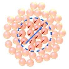
(a)     (b)

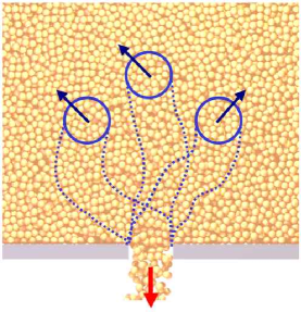
Figure 1: Spots as carriers of plastic deformation in granular materials. Cartoon of basic spot motion. A spot of local fluidization, carrying some free volume, moves to the upper right causing a cooperative displacement of particles, to the lower left, opposing the spot displacement. (b) In silo drainage, spots are injected at the orifice and perform random walks biased upward by gravity, causing downward motion of particles.

Based on this evidence for correlated motion, Bazant constructed the Spot Model for random packing dynamics and applied it to the case of granular drainage [4]. The model is based on a collective microscopic mechanism for flow, where particles move to oppose the random motion of “spots”, as depicted in Figure 1. When a spot displaces, the nearby affected particles respond by displacing in a block-like fashion in the opposite direction. The spot can thus be viewed as effectively carrying free volume and would typically be associated with a slight increase in the local interstitial volume of the packing. As a first approximation, identical spots undergo independent random walks through the material, although interactions between spots (e.g. carried by the stress field) and statistical variations in spot size and shape could be considered as well.

Each step of its random trajectory, a spot chooses the displacement $\Delta\mathbf{x}_{s}$ following a biased random process. The mean displacement, which is effectively the deterministic part of the motion, is given by

$$\left\langle\Delta\mathbf{x}_{s}\right\rangle=\Delta t\mathbf{D}_{1}$$ (1)

for step duration $\Delta t$ and drift vector $\mathbf{D}_{1}$. The random part of the motion can be described at the simplest level by

$$\left\langle\Delta\mathbf{x}_{s}\otimes\Delta\mathbf{x}_{s}\right\rangle=2\Delta t\mathbf{D}_{2}$$ (2)

where $\mathbf{D}_{2}$ is the symmetric tensor of diffusion coefficients (co-variance matrix) measuring the random fluctuations in each direction. These coefficients suffice to construct a continuous Fokker-Planck (drift-diffusion) equation to approximate the spot concentration,

$$\frac{\partial\rho_{s}}{\partial t}+\mbox{\boldmath{$\nabla$}}\cdot(\mathbf{D}_{1}\rho_{s})=(\mbox{\boldmath{$\nabla$}}\otimes\mbox{\boldmath{$\nabla$}}):(\mathbf{D}_{2}\rho_{s})+\ldots$$ (3)

where omitted correction terms (in the Kramers-Moyall expansion) depend on higher moments of the spot displacement [29]. For example, in a simple model of silo drainage (ressembling the classical kinematic [27] and void [17, 24] models), the drift vector may be chosen to point uniformly upward, since particles drift downward due to gravity, with a constant diffusivity tensor to obtain spot trajectories as sketched in Figure 1(b).

In steady-state flow, the spot concentration satisfies the time-independent drift-diffusion equation,

$$\mbox{\boldmath{$\nabla$}}\cdot(\mathbf{D}_{1}\rho_{s})=(\mbox{\boldmath{$\nabla$}}\otimes\mbox{\boldmath{$\nabla$}}):(\mathbf{D}_{2}\rho_{s})$$ (4)

where $\mathbf{A}:\mathbf{B}=A_{ij}B_{ij}$. Once solved, the mean particle velocity field $\mathbf{u}$ can be found by superposing the effects of all spots on all the particles. This is easiest to see as a convolution of some influence function $w(\mathbf{r},\mathbf{r}^{\prime})$, representing the amount of influence a spot centered at $\mathbf{r}^{\prime}$ has on a particle at $\mathbf{r}$, and the negative spot flux vector

$$\mathbf{u}^{*}=-\mathbf{D}_{1}\rho_{s}+\mbox{\boldmath{$\nabla$}}\cdot(\mathbf{D}_{2}\rho_{s}).$$ (5)

Thus the particle velocity $\mathbf{u}$ is

$$\mathbf{u}=\int w(\mathbf{r},\mathbf{r}^{\prime})\mathbf{u}^{*}(\mathbf{r}^{\prime})d\mathbf{r}^{\prime}.$$ (6)

The influence function, which in simple language describes the spot’s shape, should have a characteristic width of three to five particle diameters, so that spots match known correlation length data. In many situations, $\mathbf{u}^{*}$ is close to $\mathbf{u}$ since the convolution with $w$ tends only to smooth out sharp changes in the spot flux density.

There are several ways to use the multiscale description of the Spot Model, as have been demonstrated in the case of silo drainage. Given the drift field $\mathbf{D}_{1}$, diffusion tensor field $\mathbf{D}_{2}$, and for extra clarity the spot influence function $w$, equations (4) and (6) could be solved analytically or numerically to give the mean flow field; the statistical trajectories of particles could also be constructed, thus linking particle diffusion to the diffusion of free volume [4]. The microscopic basis for the Spot Model, however, also allows for explicit multiscale simulations of all particles in a granular flow, alternating between mesoscopic spot displacements and cooperative particle motion; this approach yields remarkably realistic flowing packings (compared to DEM simulations) in silo drainage [30]. This suggests that the spot mechanism provides a robust description of how granular flow occurs and could apply in a more universal sense, beyond just the gravity driven drainage from a silo.

The difficult question, if we want to extend the spot model to an arbitrary environment, is how can we derive the spot dynamics (or at least $\mathbf{D}_{1}$ and $\mathbf{D}_{2}$) from mechanical principles? The intuition behind the simple spot dynamics in silo drainage has no clear extension to other situations, such as an annular Couette cell, where the flow is unaffected by gravity. Instead, the spot dynamics must be related to stresses in the material, not only due to body forces, but also due to forces transmitted from moving boundary tractions.

2.2 Quasi-static granular stresses

In a dense granular material, forces are transmitted across discrete contact networks, which can be rather complicated and varying at the same length scale as the velocity profile or even the container geometry. Even the simplest question of how forces are transmitted in static granular heaps has been the subject of considerable controversy [6, 10, 22, 35, 15]. Nevertheless, it seems reasonable that a continuum theory could at least describe the mean stress state in a steady flow as a starting point for applying the SFR. Some of the random fluctuations in the force network could also be manifested in the random motion of spots coupled to mean stresses.

Most common continuum theories for solid-like material that can plastically flow utilize some type of elasticity, generating the stress tensor $\mathbf{T}$ from a small elastic strain $\mathbf{E}^{e}$ via $\mathbf{T}=\mathscr{C}[\mathbf{E}^{e}]$ where the fourth rank tensor function $\mathscr{C}$ is determined by the chosen elasticity formulation. Elliptic systems of equations, such as the laws of linear isotropic elasticity, have solutions for any given set of boundary tractions or displacements, and thus complete boundary data must be supplied.

This is problematic for granular materials since the boundary stresses in a static assembly are frequently the quantity of interest. For example, the pressure distribution under a sand-pile or the wall stresses in a bin have both been studied extensively, as noted above. Static granular boundary conditions typically develop internally as a response to the construction proceedure and often cannot be fluctuated without plastically deforming the assembly.

Hyperbolic laws of stresses have the benefit of constraint: if the tractions along one boundary region are chosen, their effect can propagate through the bulk to other boundaries and place constraints on the allowable tractions there. Some non-linear elasticity laws have been shown to yield unique solutions under restrained boundary information [13], but it appears a different continuum approach may be more naturally suited for granular materials.

The traditional approach from soil mechanics is not a strain-based stress formulation, but rather an analysis based more closely on a yield function. The Coulomb yield function defines failure whenever $\left|\tau/\sigma\right|=\mu=\tan\phi$ where $\tau$ is the shear stress on a plane, $\sigma$ the normal stress, and $\mu$ is an internal friction coefficient unique to the material. This yield function akin to a cohesionless dry friction law seems the natural choice for a continuum description of granular materials—applying higher compression locks the grains more securely, and thus makes it harder to shear them. Our experience with granular piles also direct us to this yield function. If we pour sand from a narrow spout onto a rough table, grains build up on the surface of the sand cone until the cone angle reaches a certain value at which point grains always slide down the surface, analogous to how a frictional block resting on a board will start to slide if the board is tilted above some critical angle.

In the Critical State Theory of soils [33], the stresses throughout a moving soil eventually converge onto a “critical state line” where pressure $p$ and stress deviator $q$ are linearly related. This locus strongly resembles the Drucker-Prager yield criterion, a simplified Coulomb yield law for 3D. The deformation rate in such slow flows does not significantly contribute to the stress state.

For this and other reasons we too will adopt a rate-independent formulation for granular stresses, which should owe well to the slow flowing regime we are primarily concerned with. To connect the flowing to the static regime, a common assertion is that the yield criterion is being met at all points in the material whether or not the material is flowing yet [26]. When static material is brought to steady motion under this assertion, the locus of static stresses already resembles the critical state line and thus no new stress laws are needed.

Materials obeying this traditional hypothesis are said to be at limit-state. Let us focus entirely on 2D geometries (plane strain) complete with a 2D stress tensor $\mathbf{T}$ defined in the plane of the flow. By requiring the yield criterion to be met at all points, the limit-state assumption implies the following constraint $\frac{1}{\sqrt{2}}\left|\mathbf{T}_{0}\right|=\sin\phi\left(\frac{1}{2}\operatorname{tr}\mathbf{T}\right)$ where $\mathbf{T}_{0}$ is the deviatoric stress tensor and $\left|\mathbf{A}\right|=\sqrt{\mathbf{A}:\mathbf{A}}$. A simple way to uphold this constraint is to rewrite the stress field in terms of two stress parameters (the Sokolovskii variables [36]): $p$ the average pressure, and $\psi$ the so-called “stress-angle” denoting the angle from the horizontal to the major principal stress. The components of the 2D stress tensor are then

$$T_{xx} = -p(1+\sin\phi\cos 2\psi)$$ (7)

$$T_{yy} = -p(1-\sin\phi\cos 2\psi),$$ (8)

$$T_{xy}=T_{yx} = -p\sin\phi\sin 2\psi$$ (9)

from which it can be seen that $p=-\operatorname{tr}\mathbf{T}/2$ and $\tan 2\psi=2T_{12}/(T_{11}-T_{22})$. The convection-free 2D momentum balance law $\mbox{\boldmath{$\nabla$}}\cdot\mathbf{T}+\mathbf{F}_{\textrm{body}}=\mathbf{0}$ then reduces to the two variable system of hyperbolic PDEs

$$(1+\sin\phi\cos 2\psi)p_{x}-2p\sin\phi\sin 2\psi\ \psi_{x}+\sin\phi\sin 2\psi\ p_{y}+2p\sin\phi\cos 2\psi\ \psi_{y} = F_{\textrm{body}}^{x}$$ (10)

$$\sin\phi\sin 2\psi\ p_{x}+2p\sin\phi\cos 2\psi\ \psi_{x}+(1-\sin\phi\cos 2\psi)p_{y}+2p\sin\phi\sin 2\psi\ \psi_{y} = F_{\textrm{body}}^{y}.$$ (11)

A simple Mohr’s circle analysis shows that the directions along which the yield criterion is met, the slip-lines, form at the angles $\psi\pm\epsilon$ from the horizontal where $\epsilon=\pi/4-\phi/2$.

2.3 The stochastic flow rule

To obtain flow from these stress equations, we will describe an unorthodox, yet effective, “stochastic flow rule” (SFR) based on postulating spot dynamics driven by local stress imbalances [14]. Unlike classical flow rules in plasticity which assume an ideal continuous medium, the SFR reflects the discreteness and randomness inherent to a granular packing. In its simplest embodiment, the SFR provides a unique way of defining the spot drift $\mathbf{D}_{1}$ and diffusivity $\mathbf{D}_{2}$ in an arbitrary plane strain environment.

The SFR is based physically on the notion that spots move by sliding on average along the (Mohr-Coulomb) slip-lines. However, there are two crucial sources of randomness: The slip-lines themselves are blurred by statistical fluctuations [28], but, more fundamentally, the spot must randomly decide between one of two slip-lines through each material point to slide in each step. Given the discrete nature of the packing at the spot scale (several particle diameters), it would be geometrically impossible for the spot to cause particle displacements along both slip-lines at once.

In principle, the SFR is very general and could apply to any limit-state stress field (not only for a granular material), but to arrive at the simplest possible model for granular flow, with only one parameter, we make several bold assumptions. The first is that of isotropic spot diffusion $\mathbf{D}_{2}=D_{2}\mathbf{1}$ which may be justified to some extent by slip-line blurring. To determine the magnitudes of the drift and diffusion, we reason qualitatively. A spot can be viewed as a local region of internal plastic failure, which perturbs the contact stresses on neigboring material elements. Such a perturbation can incite adjacent material to fail and when it does, the spot effectively propagates to a new location. For a typical spot size $L_{s}$, the distance of propagation should thus be roughly $L_{s}$ as well. Accordingly, we constrain all lengths referenced in the definitions of the drift and diffusion, equations (1) and (2), to uphold this notion, i.e. $\left|\mathbf{D}_{1}\right|=L_{s}/\Delta t$, and $D_{2}=L_{s}^{2}/2\Delta t$. All that remains is to determine the drift direction $\hat{\mathbf{d}}_{s}=\mathbf{D}_{1}/\left|\mathbf{D}_{1}\right|$, which is where stresses enter the model.

We derive the spot drift from local stress imbalances upon fluidization as follows (see [14] for more details). Define a material cell as the roughly diamond-shaped region encompassed by two intersecting pairs of slip-lines, separated by $L_{s}$. If a spot enters a cell, the value of the internal friction along the cell boundaries should drop from $\mu$ to the kinetic value $\mu_{k}$ causing a change in the shear tractions. This fluctuation may generate a net force on the cell, which takes the simple form,

$$\mathbf{F}_{\textrm{net}}=\left(1-\mu_{k}/\mu\right)(\mathbf{F}_{\textrm{body}}-\cos^{2}\mbox{\boldmath{$\nabla$}}p).$$ (12)

This force pushes the material one way, and consequently a spot should move the other. Since there is a slip-line field, however, a spot cannot move in any arbitrary direction. Instead, the motion opposing the net force must be projected onto slip-lines to obtain allowable motions. By projecting $-\mathbf{F}_{\textrm{net}}$ onto the slip-lines and averaging, we find that the spot drift direction is given by

$$\mathbf{\xi^{\pm}} = -(\mathbf{F}_{\textrm{net}}\cdot\mathbf{\hat{n}_{\psi\pm\epsilon}})\mathbf{\hat{n}_{\psi\pm\epsilon}}$$ (13)

$$\hat{\mathbf{d}}_{s} = \frac{\mathbf{\xi^{+}}+\mathbf{\xi^{-}}}{\left|\mathbf{\xi^{+}}+\mathbf{\xi^{-}}\right|}$$ (14)

With these assumptions, the SFR is specified enough for multiscale simulations, alternating between continuum stress computation, mesoscale spot random walks, and cooperative particle displacements. Alternatively, as a continuum approximation, the mean flow profile can be constructed by a two-step process:

1. Calculate the steady spot concentration the drift-diffusion equation, which now has the simplified form

   $$\mbox{\boldmath{$\nabla$}}\cdot(\hat{\mathbf{d}}_{s}\rho_{s})=\frac{L_{s}}{2}\mbox{\boldmath{$\nabla$}}^{2}\rho_{s}.$$ (15)

2. Compute the mean particle velocity by convolving the spot influence function with the reversed spot flux,

   $$\mathbf{u}=-\frac{L_{s}}{\Delta t}\int w(\mathbf{r},\mathbf{r}^{\prime})\left(\hat{\mathbf{d}}_{s}(\mathbf{r}^{\prime})\rho_{s}(\mathbf{r}^{\prime})-\frac{L_{s}}{2}\mbox{\boldmath{$\nabla$}}\rho_{s}(\mathbf{r}^{\prime})\right)d\mathbf{r}^{\prime}.$$ (16)

As can be seen from above, the spot step duration $\Delta t$ has no effect on the flow profile, aside from a simple rescaling of the velocity. Together with the fact that equation (15) is homogeneous in $\rho_{s}$, we observe a consequence of the SFR common to other rate-independent models: Any velocity field which solves the SFR equations is unique only up to a multiplicative constant.

3 Solving for Flow in Simple Geometries

The SFR, with some theoretical exceptions as detailed in [14], may apply as a general law in 2D plasticity. We will focus on two canonical cases which represent two very different types of granular flow: gravity-driven drainage from a silo and forced shear flow in an annular Couette cell. We are not aware of any other model, continuum or discrete, which can describe both of these cases, even qualitatively, so this will be a stringent test of the SFR. We emphasize there will be no fitting parameters used. The parameters $\phi$ and $L_{s}$ are independently measured material properties, and their values are assumed not to depend on the flow environment.

3.1 Silo

For a wide, 2D silo with smooth walls and a flat bottom, the stress balance equations can be solved analytically, giving

$$\psi=\frac{\pi}{2},\ \ \ \ \ p=\frac{f_{g}(z_{m}-z)}{1+\sin\phi}$$ (17)

where $z$ is the distance from the silo bottom, $z_{m}$ is the distance from the bottom to the free surface, and $f_{g}$ is the material’s weight density. Applying equation (12) gives $\mathbf{F}_{\textrm{net}}$ pointing uniformly downward and thus $\hat{\mathbf{d}}_{s}=\mathbf{\hat{z}}$. To visualize the stress field (via its slip-lines) simultaneously with the spot drift vector, see Figure 2(a). As such, the spot concentration solves

$$\frac{\partial\rho_{s}}{\partial z}=\frac{L_{s}}{2}\mbox{\boldmath{$\nabla$}}^{2}\rho_{s}.$$ (18)

For the narrowest possible silo opening, we have the boundary condition that $\rho_{s}(x,0)=\delta(x)$. In line with our intuition on jammed states, this implies the opening must be at least one spot width for any flow to occur. Solving with a Fourier transform gives [14]

$$\rho_{s}\approx\frac{\exp(-x^{2}/4bz)}{\sqrt{4\pi bz}}$$ (19)

for $b=L_{s}/2$ and consequently, by substituting $\rho_{s}$ into equation (5), we have $\mathbf{u}^{*}\cdot\mathbf{\hat{z}}\propto-\frac{\exp(-x^{2}/4bz)}{\sqrt{4\pi bz}}$.

Since the velocity gradient should not rapidly fluctuate in the bulk flow region we are interested in, we utilize $\mathbf{u}\approx\mathbf{u}^{*}$. Diffusive spreading of the downward velocity, as predicted here, is a well-documented phenomenon in silo drainage [27, 32, 8, 37, 20]. Utilizing the $L_{s}$ dependence, the typical range of $b$ values is predicted to be $1.5d$ to $2.5d$ which compares quite well to the results of documented experiments on silo diffusion which, when accumulated, give a total $b$ range of $1.3d$ to $3.5d$. To our knowledge, there is no other theory to predict $b$, even qualitatively, from basic mechanical principles, so this should be viewed as a first success of the SFR.

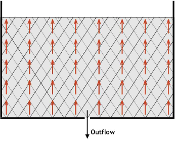
(a)               (b)

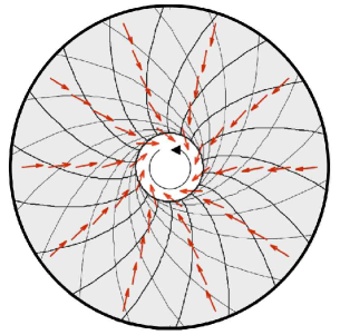
Figure 2: Slip-lines fields (from MCP) and the spot drift field (from the SFR) displayed for (a) a wide silo draining under gravity, and (b) shearing in an annular Couette cell (no gravity).

3.2 Annular Couette cell

A much stronger test of the SFR comes from its ability to adapt to a completely different flow environment, without changing any parameters. In annular Couette flow, material fills the region between two rough cylinders and is sheared by rotating the inner cylinder while holding the outer stationary. To solve for the MCP stresses, we first convert the stress balance equations to polar coordinates $(r,\theta)$ and require that $p$ and $\psi$ obey radial symmetry. This simplifies to

$$\frac{\partial\psi^{*}}{\partial r}=-\frac{\sin 2\psi^{*}}{r(\cos 2\psi^{*}+\sin\phi)},\ \ \ \ \ \frac{\partial\eta}{\partial r}=-\frac{2\sin\phi}{r(\cos 2\psi^{*}+\sin\phi)}$$ (20)

where $\eta=\log p$ and $\psi^{*}=\psi+\frac{\pi}{2}-\theta$. We solve these equations numerically using fully rough inner wall boundary conditions $\psi^{*}(r_{w})=\frac{\pi}{2}-\epsilon$ and any arbitrary value for $\eta(r_{w})$. We find that $p$ decreases with distance from the inner wall, implying $\mathbf{F}_{\textrm{net}}$ points radially outward. Applying equations (13) and (14) gives a drift field that points inward, but gradually opposes the motion of the inner wall.

Below, we solve for $\mathbf{u}^{*}$ directly by enforcing that the flow point along $\mathbf{\hat{\theta}}$. Since the material near the wall shears rapidly, we cannot assert $\mathbf{u}\approx\mathbf{u}^{*}$ and must solve the full convolution, equation (6). For simplicity, we assume circular spots $w(\mathbf{r},\mathbf{r}^{\prime})\propto H(\frac{L_{s}}{2}-\left|\mathbf{r}-\mathbf{r}^{\prime}\right|)$ where $H$ is a step function. (Velocity correlations measurements in silo experiments suggest that the spot shape may be anisotropic due to gravity, or more generally, local stresses, but this is not a major effect [14].) To properly describe particle motion near the wall, we must decide how spots interact with walls so that the convolution integral can be carried out all the way to the inner wall. A simple claim is that $\mathbf{u}^{*}$ must equal the wall velocity wherever spots overlap the wall—a no-slip condition of sorts. After convolution, the net effect of this assertion is that $\mathbf{u}$ is slightly flatter than $\mathbf{u}^{*}$ close to the inner wall. We shall refer to this assumption about wall interactions as “wall hypothesis 1”. We note that this is slightly different than the hypothesis used in [14] which claims the region within the walls can be viewed as a bath of non-diffusive spots which cause particles to move in a manner that mimics the rigid wall motion. We shall refer to this as “wall hypothesis 2”. Though our theory is flexible in terms of near wall specificities, the bulk behavior, regardless of which hypothesis is selected, is always the same.

4 Comparing SFR Predictions to Discrete Element Simulations

4.1 Simulation Methods

To test the above models, we carried out DEM simulations using a modified version of the Large-scale Atomic/Molecular Massively Parallel Simulator (LAMMPS) developed at Sandia National Laboratories [1]. Following a similar approach to previous work by our group [30, 31] and others [34, 15] we considered simulations of spherical particles interacting using a modified version of the model developed by Cundall and Strack [11] to model cohesionless particulates. Monodisperse spheres with diameter $d$ interact according to Hertzian, history dependent contact forces. For a distance $\mathbf{r}$ between a particle and its neighbor, when the particles are in compression, so that $\delta=d-\left|\mathbf{r}\right|>0$, then the two particles experience a force $\mathbf{F}=\mathbf{F}_{n}+\mathbf{F}_{t}$, where the normal and tangential components are given by

$$\mathbf{F}_{n}=\sqrt{\delta/d}\left(k_{n}\delta\mathbf{n}-\frac{\gamma_{n}\mathbf{v}_{n}}{2}\right),\ \ \ \ \mathbf{F}_{t}=\sqrt{\delta/d}\left(-k_{t}\Delta\mathbf{s}_{t}-\frac{\gamma_{t}\mathbf{v}_{t}}{2}\right).$$ (21)

Here, $\mathbf{n}=\mathbf{r}/\left|\mathbf{r}\right|$. $\mathbf{v}_{n}$ and $\mathbf{v}_{t}$ are the normal and tangential components of the relative surface velocity, and $k_{n,t}$ and $\gamma_{n,t}$ are the elastic and viscoelastic constants, respectively. $\Delta\mathbf{s}_{t}$ is the elastic tangential displacement between spheres, obtained by integrating tangential relative velocities during elastic deformation for the lifetime of the contact, and is truncated as necessary to satisfy a local Coulomb yield criterion $\left|\mathbf{F}_{t}\right|\leq\mu_{c}\left|\mathbf{F}_{n}\right|$. Particle-wall interactions are treated identically, though the particle-wall friction coefficient $\mu_{w}$ is set independently.

For the current simulations we set $k_{t}=\frac{2}{7}k_{n}$, and choose $k_{n}=2\times 10^{5}mg/d$. This is significantly less than would be realistic for many hard granular materials, such as glass beads, where we expect $k_{n}>10^{10}mg/d$, but such a spring constant would be prohibitively computationally expensive, as the time step scales as $\delta t\propto k_{n}^{-1/2}$ for collisions to be modeled effectively. Previous simulations have shown that increasing $k_{n}$ does not significantly alter physical results [15]. We use a time step of $\delta t=1.0\times 10^{-4}\tau$ and damping coefficients $\gamma_{n}=50\tau^{-1}$ and $\gamma_{t}=0.0$. All measurements are expressed in terms of $d$ and $\tau$. We make use of both cartesian coordinates $(x,y,z)$ and cylindrical coordinates $(r,\theta,z)$ where $r^{2}=x^{2}+y^{2}$; gravity is set to $1d\tau^{-2}$ and points in the negative $z$ direction.

The simulations were carried out on MIT’s Applied Mathematics Computational Laboratory, a Beowulf cluster consisting of 16 nodes each with a dual processor. During the simulations, snapshots of all particle positions were saved every $2\tau$, corresponding to 20000 integration timesteps. The LAMMPS code is written in C++ and can be run on any number of processors, by decomposing the computational domain into cuboidal subdomains of equal size. Interactions between particles in neighboring domains are handled using message passing. For problems where the particles are split evenly between the subdomains, the LAMMPS code scales very well, and doubling the number of processors can frequently result in almost a doubling of speed. However, the Couette geometry causes some subdomains to have more particles than others, leading to poor load-balancing. Most of the simulations were therefore run on four processors, with the domains split by the planes $x=0$ and $y=0$ to achieve optimal load-balancing; these simulations took approximately four weeks to complete.

4.2 The silo geometry

We considered a quasi-2D silo with plane walls at $x=\pm 75d,z=0$ with friction coefficient $\mu_{w}=0.5$, and made the $y$ direction periodic with width $8d$. To generate an initial packing, $90,000$ spherical particles with contact friction coefficient $\mu_{c}=0.5$ were poured in from a height of $z=130d$ at a rate of $378\tau^{-1}$. After all particles are poured in at $t=238\tau$, the simulation is run for an additional $112\tau$ in order for the particles to settle. After this process has taken place, the particles in the silo come to a height of approximately $z=62.2d$. To initiate drainage, an orifice in the base of the container is opened up over the range $-3d<x<3d$, and the particles are allowed to fall out under gravity; Figure 3(a) shows a typical simulation snapshot during drainage.

As noted in the previous section, snapshots of the particle positions are saved every $2\tau$. We collected $282$ snapshots, and made use of this information to construct velocity cross sections. A particle with coordinates $\mathbf{x}_{n}$ at the $n$th timestep and $\mathbf{x}_{n+1}$ at the $(n+1)$th timestep makes a velocity contribution of $(\mathbf{x}_{n+1}-\mathbf{x}_{n})/\Delta t$ at the point with coordinates $(\mathbf{x}_{n}+\mathbf{x}_{n+1})/2$. This data can then be appropriately binned to create a velocity profile; we considered bins of size $d$ in the $x$ direction, and created velocity profiles for different vertical slices $\left|z-z_{s}\right|<d/2$.

Since the SFR makes predictions about the velocity profile during steady flow, we choose a time interval $t_{1}<t<t_{2}$ over which the velocity field is approximately constant. Choosing this interval requires some care, since if $t_{1}$ is too small then initial transients in the velocity profile can have an effect, and if $t_{2}$ is too large, then the free surface can have an influence. For the results reported here, we chose $t_{1}=120\tau$ and $t_{2}=200\tau$.

Figure 3(b) compares the SFR predictions for this environment to the DEM simulation. The displayed simulation data uses a particle contact friction of $\mu_{c}=0.3$. Since the typical range of $L_{s}$ from velocity correlations in simulations [30] and experiments [14] is $3d$ to $5d$, we choose $L_{s}=4d$ to generate the approximate SFR solution. We emphasize that this parameter is not fitted. In this geometry, the slip-lines are symmetric about the drift direction causing both $\mathbf{D}_{1}$ and $D_{2}$ to become independent of the internal friction. In prior simulations we have found that that particle contact friction has some effect on the flow [31], and analogously the internal friction should play some role in the determination of $b$. Here, the loss of friction dependence comes from our simplification that $\mathbf{D}_{2}$ is isotropic. A less simple but more precise definition for $\mathbf{D}_{2}$ would anisotropically skew the spot diffusion tensor as a function of internal friction: the slip-lines, which we model as the directions along which a spot can move (roughly), intersect at a wider angle as internal friction is increased.

Even so, our simple model captures many of the features of the flow and accurately portrays the dominant behavior. The downward velocity, especially at $z=10d$, strongly matches the predicted Gaussian. Perhaps a more global demonstration of the underlying stochastic behavior in the SFR is evident in Figure 3(c), where a linear relationship can be seen between the mean square width of $v_{z}$ and the height, indicating that the system variables are undergoing a type of diffusive scaling. The SFR solution also predicts this linear relationship and, in particular, that the slope should equal $2b=L_{s}$. The agreement shown in Figure 7(b) for such a typical $L_{s}$ value is a strong indicator that the role of the correlation length in the flow has been properly accounted for in the SFR.

The diffusive velocity profile near the orifice of a wide silo has also been observed in a number of experiments [25, 37, 19, 32] and DEM simulations [30, 31] and was first predicted qualitatively by kinematic models [17, 24, 27]. Such models, however, lack a plausible microscopic basis [4] or any connection with mechanics and cannot be applied to any other geometry, other than the wide silo.

(a)

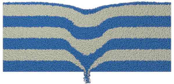
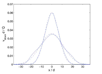
(b) (c)

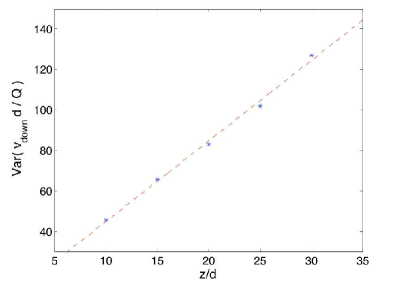
Figure 3: (a) A typical snapshot of the silo system during drainage, taken at $t=60\tau$. The colored bands are initially spaced $10d$ apart, and highlight the deformations that occur during flow (b) Mean downward velocity profiles at two different heights in a wide silo. DEM results (solid lines) are plotted against the SFR predictions (dashed lines) at heights of $z=10d,30d$; (c) Mean square width of the downward velocity across horizontal cross-sections in the DEM (points), compared to the SFR (dashed line)

4.3 The Couette geometry

For the Couette geometry, we considered five different interparticle friction coefficients, $\mu_{c}=0.1,0.3,0.5,0.7,0.9$, and for each value an initial packing was generated using a process similar to that for the silo. We consider a large cylindrical container with a side wall at $r=64d$ with friction coefficient $\mu_{w}=\mu_{c}$, and a base at $z=0$ with friction coefficient $\mu_{w}=0$. For each simulation, 160000 particles are poured in from a height of $z=48d$ at a rate of $4848\tau^{-1}$. After all particles are introduced at $t=33\tau$, the simulation is run for an additional time period of $322\tau$ to allow the particles to settle. After this process has taken place, the initial packings are approximately $11.5d$ thick. Packings with $\mu_{c}=0.9$ are approximately $2\%$ thicker than those with $\mu_{c}=0.1$.

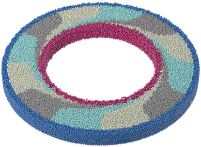
(a)  (b)

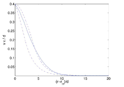
Figure 4: (a) A typical snapshot of the system during shearing based on the simulation with $r_{\textrm{in}}=40d$, $\omega=0.01\tau^{-1}$, and $\mu_{c}=0.5$. Dark blue particles (with $r>r_{\textrm{out}}$) are frozen during the simulation, while dark red particles (with $r<r_{\textrm{in}}$) are rotated with angular velocity $\omega$. The particles between $r_{\textrm{in}}$ and $r_{\textrm{out}}$ undergo shearing. The colored bands of grey, cream, and cyan were initially radial, and in this snapshot, after fifty frames, the deformations can be clearly seen. (b) SFR solutions using wall hypothesis 1 (dashed line) and wall hypothesis 2 (dot-dashed line) in the annular Couette geometry ($r_{\textrm{in}}=40d,r_{\textrm{out}}=60d$) are compared to the simulation results (solid line). Both use the same parameters that were used in the silo geometry ($L_{s}=4d,\mu_{c}=0.3$) and the bead internal friction angle is set at the typical value $25^{o}$.

The shearing simulations take place in an annulus between two radii, $r_{\textrm{in}}$ and $r_{\textrm{out}}$. A rough outer wall is created by freezing all particles which have $r>r_{\textrm{out}}$; any forces or torques that these particles experience are zeroed during each integration step. Similarly, all particles between $r_{\textrm{in}}-4d$ and $r_{\textrm{in}}$ are forced to rotate with a constant angular velocity $\omega$ around $r=0$. Particles with $r<r_{\textrm{in}}-4d$ are deleted from the simulation and an extra cylindrical wall with friction coefficient $\mu_{w}=\mu_{c}$ is introduced at $r=r_{\textrm{in}}-4d$ to prevent stray surface particles from falling out of the shearing region. A typical run is shown in Figure 4(a).

From the five initial packings, we carried out eight different shear cell simulations to investigate the effects of friction, angular velocity, and inner wall radius. To investigate the effect of friction, five runs were carried out with $\omega=0.01\tau^{-1}$ and $r_{\textrm{in}}=40d$, for $\mu_{c}=0.1,0.3,0.5,0.7,0.9$. To examine the effect of the inner wall radius, an additional run with $r_{\textrm{in}}=30d$ and $r_{\textrm{out}}=50d$ was carried out, with $\mu_{c}=0.3$ and $\omega=0.01\tau^{-1}$ kept constant. To look at the effect of angular velocity, a further two runs with $\omega=0.05\tau^{-1}$ and $\omega=0.2\tau^{-1}$ were carried out, with $\mu_{c}=0.5$ and $r_{\textrm{in}}=40d$ kept constant. For each simulation, we collected $561$ snapshots. For the runs where $r_{\textrm{in}}=40d$, approximately $108350$ particles were simulated, corresponding to $2.0$Gb of data. For the run with $r_{\textrm{in}}=30d$, $88657$ particles were simulated, corresponding to $1.7$Gb of data.

The simulation results show a good empirical agreement with previous experimental work on shear cells [18, 21, 16, 5, 23]. In all cases, we see an angular velocity profile that falls off exponentially from the inner cylinder, with a half-width on the order of several particle diameters. Near the inner wall, the flow deviates from exponential, which is an effect seen in some prior studies but is more dramatic here. Following methods similar to those used in silo simulation, we used the snapshots to construct an angular velocity profile. We used bins of size $d/2$ in the radial direction, and we looked at velocity profiles in different vertical slices $z_{\textrm{low}}<z<z_{\textrm{high}}$.

Since the simulation geometry is rotationally symmetric, our angular velocity profile can most generally be a function of $r$, $z$ and $t$. Ideally, we hope that $\omega$ is primarily a function of $r$, with only a very weak dependence on $z$ and $t$, but we began by studying the effects of these other variables. To determine the dependence on time, the velocity profiles were calculated over many different time intervals. As would be expected, the simulation had to be run for small amount of time before the velocity profile would form; this happens on a time scale of roughly $50\tau$, and the results suggest a longer time is needed for the cases with low friction. However, the data also shows time-dependent effect happening on a longer scale: as the shearing takes place, there is a small but consistent migration of particles away from the rotating wall, which has a small effect on the velocity profile. This effect does eventually appear to saturate, but because of this, we chose to discard the simulation data for $t<500\tau$ and calculate velocity profiles based on the time window $500\tau<t<1100\tau$.

To investigate the angular velocity dependence on the height, we calculated the velocity profiles in five different slices $z_{h}<z<z_{h}+d$ for $z_{h}=d,3d,5d,7d,9d$. Near the inner rotating wall, the velocity profiles show very little dependence on height. However, in the slow-moving region close to the fixed outer wall, large differences can be seen, with particles in the lowest slice moving approximately $30\%$ slower than those in the central slice, and those in the top slice moving approximate $30\%$ faster. The three central slices show differences of at most $10\%$, and we therefore chose to use the range $3d<z<8d$.

The SFR treats the correlation length as a material property independent of the flow geometry or other state variables. To see how well this notion is upheld, we solve the SFR in the annular Couette geometry using the same correlation length ($L_{s}=4d$) that was used in the displayed silo prediction, Figure 3. It is then compared to a simulation of annular flow which uses the same grain properties ($\mu_{c}=0.3$).

Results from Figure 4(b) show that regardless of the wall hypothesis, the SFR prediction captures the same qualitative features of the simulation. The SFR and simulation both predict a flatter range near the inner wall, followed by exponential decay. Near the inner wall, it does appear that wall hypothesis 1 (“no slip condition” for spots) gives a closer match to the simulation.

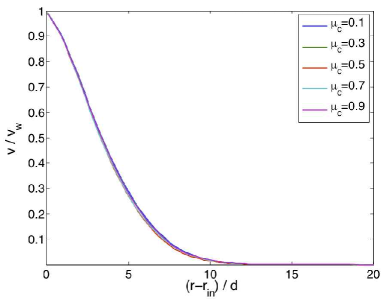
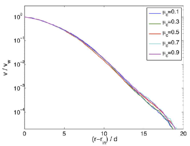
Figure 5: Velocity profiles for five different values of $\mu_{c}$, where $r_{\textrm{in}}=40d$ and $\omega=0.01\tau^{-1}$.

The SFR, when applied to the annular flow geometry, does predict a slight dependence of the flow on the internal friction. We emphasize that internal friction is not the same quantity as particle contact friction $\mu_{c}$, though we believe if the contact friction is increased, inevitably, the internal friction must be as well. Spherical grains almost always have internal friction angles in the range $\phi=20^{\circ}$ to $\phi=30^{\circ}$, so to represent this range as best as possible, we simulated flows varying the particle contact friction from $\mu_{c}=0.1$ to $\mu_{c}=0.9$. Figure 5 displays velocity profiles for five different values of friction. In the semi-log format, profiles appear almost linear over the range $45d<r<58d$ indicating a very good fit to an exponential model of velocity.

Since the curves in the figure are very close, and exhibit some experimental noise, it is difficult to discern any small differences in the widths of the velocity profiles. However, table 1 shows the results of applying linear regression to extract a half-width for each velocity profile. We see differences on the order of $5\%$, roughly in line with the SFR. More importantly, the trend of increasing flow width with increasing friction is seen in both.

When the inner wall radius is decreased, Figure 6 indicates that the shear band shrinks but the decay behavior in the tail changes only minimally. The SFR predicts this qualitative trend as well, but significantly underestimates the size of the shear-band decrease.

In agreement with past work on Couette flow [18, 5], we too find that the normalized flow profile is roughly unaffected by the shearing rate (see Figure 7). As previously discussed, this behavior is in agreement with the SFR, which always permits flow fields to be multiplied by a constant.

$\mu_{c}$	$b$
$0.1$	$0.974d$
$0.3$	$0.983d$
$0.5$	$1.033d$
$0.7$	$1.046d$
$0.9$	$1.032d$

$\phi$	$b$
$20^{\circ}$	$1.026d$
$22^{\circ}$	$1.038d$
$24^{\circ}$	$1.052d$
$26^{\circ}$	$1.069d$
$28^{\circ}$	$1.084d$
$30^{\circ}$	$1.102d$

Table 1: (Left) Simulation: Half-widths of the shearing velocity profiles for different values of $\mu_{c}$, calculated by fitting the functional form $f(r)=a-(\log 2)r/b$ to $\log v/v_{w}$ over the range $45d<r<58d$. (Right) SFR: Fits the predictions to the same form and uses $L_{s}=3d$.

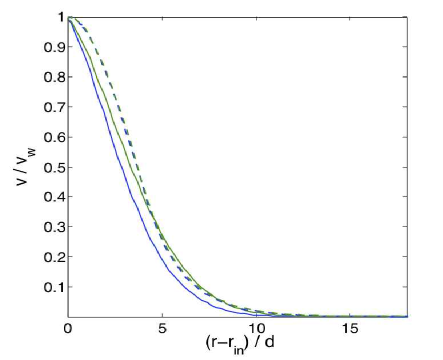
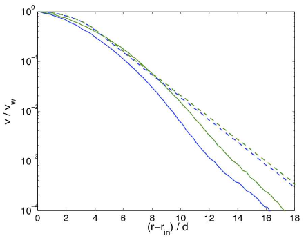
Figure 6: DEM simulation results (solid lines) for the flow profile when the inner wall radius is 30d (blue) and 40d (green) compared to SFR predictions (dashed lines) which use the same color scheme. For solidarity with the silo flow predictions, the SFR solutions use $L_{s}=4d$.

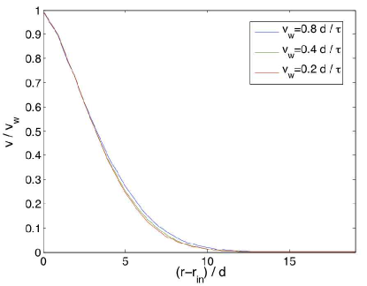
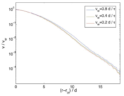
Figure 7: Velocity profiles for three different angular velocities, with $\mu_{c}=0.5$ and $r_{\textrm{in}}=40d$. The time windows over which the velocities are computed are scaled according to the angular velocity.

5 Conclusion

We have presented the crucial principles motivating the Stochastic Flow Rule and have assessed its validity by checking analytical predictions for silo and annular Couette flow against discrete-element simulations. Using the same parameters for both cases, without any fitting, the SFR manages good predictions for these two very different flow geometries, which it seems cannot be described, even qualitatively, by any other model. The model was also shown to capture the “diffusive” type flow properties unique to granular materials such as Gaussian downward velocity in the draining silo and exponentially decaying velocity in the annular Couette cell.

Our simulations also indicate that the slight changes in flow brought on by varying the inter-particle contact friction in the annular flow geometry match the trends the SFR predicts when the internal friction angle is approrpiately varied. The trend is also captured when the inner wall radius is varied, though the quantitative agreement is not as strong. In agreement with past studies on annular Couette flow, and in validation of one of the first principles behind the SFR, we find in our simulations that the flow rate does not significantly affect the normalized flow profile over a significant range of rates.

These results, taken together with our prior work on spot-driven particle simulations [30], suggest that the SFR provides a general paradigm for multiscale modeling of granular flow or, more generally perhaps, plastic deformation of other amorphous materials. Whenever the stress state is near yielding our physical picture of flow is that spots of fluidization perform random walks along slip-lines biased by local stress imbalances. With some exceptions as outlined in [14] (so-called “slip-line admissible” geometries) we believe the SFR is a highly general law for 2D dense granular flow.

References

- [1] http://lammps.sandia.gov.
- [2] I. S. Aranson and L. S. Tsimring. Patterns and collective behavior in granular media: Theoretical concepts. Rev. Mod. Phys., 78:641–692, 2006.
- [3] N.J. Balmforth and A. Provenzale. Geomorph. Fluid Mech. Springer, 2001.
- [4] M. Z. Bazant. The spot model for random-packing dynamics. Mechanics of Materials, 38:717–731, 2006.
- [5] L. Bocquet, W. Losert, D. Schalk, T. C. Lubensky, and J. P Gollub. Phys. Rev. E, 65:011307, 2001.
- [6] J.-P. Bouchaud, M. E. Cates, and P. Claudin. Stress distribution in granular media and nonlinear wave equation. J. Phys., 5:639–656, 1995.
- [7] C. S. Campbell. Ann. Rev. Fluid Mech., 22:57, 1990.
- [8] J. Choi, A. Kudrolli, and M. Z. Bazant. Velocity profile of gravity-driven dense granular flow. J. Phys.: Condensed Matter, 17:S2533–S2548, 2005.
- [9] J. Choi, A. Kudrolli, R. R. Rosales, and M. Z. Bazant. Diffusion and mixing in gravity driven dense granular flows. Phys. Rev. Lett., 92:174301, 2004.
- [10] S. N. Coppersmith, C. h. Liu, S. Majumdar, O. Narayan, and T. A. Witten. Model for force fluctuations in bead packs. Phys. Rev. E, 53:4673–4685, 1996.
- [11] P. A. Cundall and O. D. L. Strack. A discrete numerical model for granular assemblies. Geotechnique, 29:47, 1979.
- [12] H. M. Jaeger, S. R. Nagel, and R. P. Behringer. Granular solids, liquids, and gases. Rev. Mod. Phys., 68:1259–1273, 1996.
- [13] Y. Jiang and M. Liu. Granular elasticity without the coulomb condition. cond-mat/0210557.
- [14] K. Kamrin and M. Z. Bazant. A stochastic flow rule for granular materials. cond-mat/0609448.
- [15] J. W. Landry, G. S. Grest, L. E. Silbert, and S. J. Plimpton. Confined granular packings: structure, stress, and forces. Phys. Rev. E, 67:041303, 2003.
- [16] M. Latzel, S. Luding, H. J. Herrmann, D. W. Howell, and R.P. Behringer. Comparing simulation and experiment of a 2d granular couette shear device. Euro. Phys. Journ. E., 11:325–333, 2003.
- [17] J. Litwiniszyn. Statistical methods in the mechanics of granular bodies. Rheol. Acta, 2/3:146, 1958.
- [18] W. Losert, L. Bocquet, T. C. Lubensky, and J. P. Gollub. Particle dynamics in sheared granular matter. Phys. Rev. Lett., 85:1428–1431, 2000.
- [19] A. Medina, J. Andrade, and C. Trevino. Experimental study of the tracer in the granular flow of a 2d silo. Physics Letters A, 249:63–68, 1998.
- [20] A. Medina, J. A. Cordova, E. Luna, and C. Trevino. Velocity field measurements in granular gravity flow in a near 2d silo. Physics Letters A, 220:111–116, 1998.
- [21] G. D. R. Midi. On dense granular flows. Euro. Phys. Journ. E., 14:341–365, 2004.
- [22] D. M. Mueth, H. M. Jaeger, and S. R. Nagel. Force distribution in a granular medium. Phys. Rev. E, 57:3164–3169, 1998.
- [23] Daniel E. Mueth, Georges F. Debregeas, Greg S. Karczmar, Peter J. Eng, Sidney R. Nagel, and Heinrich M. Jaeger. Signatures of granular microstructure in dense shear flows. Nature, 406:385–388, 2000.
- [24] J. Mullins. Stochastic theory of particle flow under gravity. J. Appl. Phys., 43:665, 1972.
- [25] J. Mullins. Experimental evidence for the stochastic theory of particle flow under gravity. Powder Technology, 9:29, 1974.
- [26] R. M. Nedderman. Statics and Kinematics of Granular Materials. Nova Science, 1991.
- [27] R. M. Nedderman and U. Tüzün. Kinematic model for the flow of granular materials. Powder Technology, 22:243, 1979.
- [28] M. Ostoja-Starzewski. Scale effects in plasticity of random media: status and challenges. Int. J. Plasticity, 21:1119–1160, 2005.
- [29] Hannes Risken. The Fokker-Planck Equation. Springer, 1996.
- [30] C. H. Rycroft, M. Z. Bazant, G. S. Grest, and J. W. Landry. Dynamics of random packings in granular flow. Physical Review E, 73:051306, 2006.
- [31] C. H. Rycroft, G. S. Grest, J. W. Landry, and M. Z. Bazant. Analysis of granular flow in a pebble-bed nuclear reactor. Phys. Rev. E, 74:021306, 2006.
- [32] A. Samadani, A. Pradhan, and A. Kudrolli. Size segregation of granular matter in silo drainage. Phys. Rev. E, 60:7203–7209, 1999.
- [33] A. Schofield and C. Wroth. Critical State Soil Mechanics. McGraw-Hill, 1968.
- [34] L. E. Silbert, D. Ertas, G. S. Grest, T. C. Halsey, D. Levine, and S. J. Plimpton. Granular flow down an inclined plane: Bagnold scaling and rheology. Phys. Rev. E., 64:051302, 2001.
- [35] L. E. Silbert, G. S. Grest, and J. W. Landry. Statics of the contact network in frictional and frictionless granular packings. Phys. Rev. E, 66:061303, 2002.
- [36] V. V. Sokolovskii. Statics of Granular Materials. Pergamon/Oxford, 1965.
- [37] U. Tüzün and R. M. Nedderman. Experimental evidence supporting the kinematic modelling of the flow of granular media in the absence of air drag. Powder Technolgy, 23:257, 1979.