On the orientational ordering of long rods on a lattice

Abstract

We argue that a system of straight rigid rods of length $k$ on square lattice with only hard-core interactions shows two phase transitions as a function of density $\rho$ for $k\geq 7$. The system undergoes a phase transition from the low-density disordered phase to a nematic phase as $\rho$ is increased from $0$ at $\rho=\rho_{c1}$, and then again undergoes a reentrant phase transition from the nematic phase to a disordered phase at $\rho=\rho_{c2}<1$.

1 Introduction

The study of systems of long rod-like molecules in solution with only excluded volume interaction has a long history. Onsager had noted that such a system would show long-range orientational order at large enough density [1]. Flory studied a lattice model of long rod-like molecules, and based on a mean-field approximation, argued that the lattice model would also show an isotropic-nematic phase transition as a function of density [2]. Zwanzig studied a model of hard rods in the continuum, but with only a finite number of allowed orientations [3]. For the continuum problem, there is general agreement that in three dimensions, the isotropic-nematic transition occurs at large enough density, if the length-to-width ratio of the molecules is large enough [4]. In the case of two-dimensional systems of hard needles in a plane, there is no spontaneous breaking of continuous symmetry, but the high-density phase has orientational correlations that decay as a power-law [5, 6].

The situation is much less clear in the case of lattice models of straight hard rods of length $k$. The only analytically soluble case is that of dimers ($k=2$), for which it is known that the orientational correlations have an exponential decay for all densities, except the full-coverage limit, which shows power-law correlations in all dimensions [7, 8]. Power-law correlations at $\rho=1$ were also seen in numerical study on the square lattice for $k=3$[9], and $k=4$[10]. Early Monte Carlo studies of semi-flexible $k$-mers on a square lattice showed no long-range orientational order for any density or temperature [11]. DeGennes and Prost, in 1995, in their book on liquid crystals, wrote “it is not quite certain that such a lattice model, even for large $p$ (long molecule), will lead to a transition” [12]. While there has been some work on this general problem since then, the question still remains unsettled [13] .

In this paper, we present the results of our Monte Carlo study of this model on the square lattice. We find very strong numerical evidence that the system shows nematic order at intermediate densities for $k\geq 7$. We are not able to study systems near $\rho=1$ in our simulations, because the relaxation time increases very fast with density. However, there is fairly convincing numerical evidence (but no proof), that there is no long-range order at $\rho=1$, and so there must be a second phase transition as density is increased. To the best of our knowledge, this second phase-transition has not been discussed in published literature before. We estimate the critical density for the second transition. The different phases are shown schematically in Fig. 1.

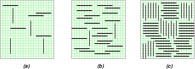
Figure 1: Schematic representation of different phases of the hard rod system on a square lattice. (a) The low-density disordered phase (b) Intermediate density ordered phase (c) the high density disordered phase.

2 Model

Our model consists of a system of hard straight rods, each of which occupies $k$ consecutive sites on a lattice. A rod has only two possible orientations, horizontal or vertical. We will call each such rod a $k$-mer. The only interaction between different rods is hard core exclusion: no site can be occupied by more than one $k$-mer.

We take the lattice to be a two-dimensional square lattice of size $L\times L$. Let $N(n_{h},n_{v})$ be the number of distinct configurations with $n_{h}$ horizontal and $n_{v}$ vertical $k$-mers. We define $z_{h}$ and $z_{v}$ as the activities for the horizontal and vertical $k$-mers, and define the grand partition function

$$\Omega(z_{h},z_{v})=\sum_{n_{h},n_{v}}N(n_{h},n_{v})z_{h}^{n_{h}}z_{v}^{n_{v}}.$$ (1)

The average values of $n_{h}$ and $n_{v}$ in the grand canonical ensemble are obtained by taking partial derivatives of $\Omega$ with respect to $z_{h}$ and $z_{v}$. We define the mean density $\rho$ as the fractional number of sites occupied by $k$-mers. The nematic order parameter $Q$ is defined as

$$Q=Lim_{z_{v}\downarrow z_{h}}Lim_{L\rightarrow\infty}\frac{\langle n_{v}-n_{h}\rangle}{\langle n_{v}+n_{h}\rangle},$$ (2)

where the limit is taken with $z_{v}$ tending to $z_{h}$ from above. We will usually be interested in the case $z_{v}=z_{h}$, and denote the common value by $z$ without a subscript.

3 Results of the Numerical Simulations

Figure 2: Snapshots of time evolution of $k$-mers, $k=8$, to the nematically ordered state for $p=.8$, starting from an empty lattice . Initially, the algorithm produces a disordered state, which slowly relaxes to the almost perfectly orientationally ordered state. The frames a-f are taken after $1000,4000,8000,12000,20000$ and $36000$ MCS. The asymptotic value of the order parameter is $Q=0.989$ and density, $\rho=0.758$.

We have studied this problem by Monte Carlo simulations using a deposition-evaporation algorithm: At each time-step, we make an attempt to deposit a rod with probability $p$, or evaporate one of the existing rods with probability $1-p$. If it is a deposition attempt, we choose a horizontal or vertical orientation with probability $1/2$ each, and pick one of the sites of the lattice at random, and attempt to deposit the rod there in the chosen direction. The attempt is successful if that site, and the next $k-1$ sites in the chosen direction are all empty. Otherwise, the attempted move is rejected. We use period boundary conditions in both the horizontal and vertical directions. It is easy to see that this deposition-evaporation dynamics is ergodic and satisfies detailed balance, with the parameter $p$ related to activity $z$ by

$$z=\frac{\rho~{}p}{2k(1-p)}.$$ (3)

The deposition-evaporation dynamics does not conserve the number of rods, $n$ and the number of vertical and horizontal rods $n_{v}$ and $n_{h}$ vary with time. In our Monte Carlo studies, we studied different values of $k$, from $2$ to $12$. We varied the deposition rate $p$ and monitored the density $\rho$ and the order parameter $Q$.

Our main result is the evidence for existence of a orientationally ordered phase for intermediate densities of rods for $k\geq 7$. The existence of the nematic phase is very clearly established in our simulations. A typical run is shown in Fig. 2, where we have taken $k=8$, on a $80\times 80$ lattice, for $p=0.8$, starting from all empty initial state. In the beginning, both horizontal and vertical deposition events are equally likely, and the density builds up to nearly equilibrium value $\simeq.75$, but the order parameter $Q$ remains nearly zero. By the time $1000$ MCS, the density has nearly stabilized to its equilibrium value, but the order parameter is nearly zero. With time, the size of locally ordered domains grow, until one of the domains nearly fills the full lattice. For our lattice, this happens by around $16000$ MCS. At this stage, the order parameter is nearly $1$, and it shows only very small fluctuations away from this value for the full length of simulation ( about $10^{7}$ MCS). The average value of $Q$ in this run was $0.989$. Of course, the ordering is equally likely to be horizontal or vertical.

We have tested the results for different initial configurations, namely, all empty, all vertical, all horizontal, half filled, etc. to ensure sufficient time has been given for equilibration, and the averages calculated are independent of initial conditions.

Figure 3: Order parameter $Q$ as a function of densities $\rho$ is shown for different $k$ and $L$.

In Fig. 3 we show that the order parameter $Q$ as a function of density $\rho$ for different length of rods $k=6,7,8,10$ and two system sizes $L=90$ and $120$. We did not find any isotropic-nematic transition for short rods $k\leq 6$. However, as our simulations only cover the range $0\leq\rho\leq.85$, we can only conclude that if $k_{min}$ the lowest value of $k$ that shows a nematic phase, then $k_{min}\leq 7$.

For long rods $k\geq 7$, a nematic phase is observed for intermediate densities. The critical density for the onset of nematic order decreases with increasing $k$. This is consistent with the theoretical expectation that for very large $k$, the critical density should be related to that found in the problem of ultra-thin needles in a continuum. If the critical density of needles of length $1$ in continuum is $A_{c}$, the critical density for the isotropic to nematic transition $\rho_{c1}$ should be approximately equal to $A_{c}/k$, for large $k$ [$A_{c}\approx 6$, from simulations].

Figure 4: Normalized distribution of $n_{v}-n_{h}$ for $k=10$ and $L=120$ is shown for different values of densities $\rho$.

The point of onset of the nematic order is not so easy to determine from the data. In Fig. 4 we show the distribution of $n_{v}-n_{h}$ for $k=10$ and $L=120$ for different densities $\rho$. For $\rho<0.36$ the distribution is centered around 0 implying that there is no preferred orientation in the configurations and that the system is in isotropic phase. While $\rho>0.4$, the distribution shifts to the right indicating onset of a nematic phase. Also, the order parameter increases gradually, indicating a continuous phase transition. Since we are not able to determine the critical point with very good precision, we did not attempt to study the critical exponents characterizing the transition. As there are two competing ordered states near the transition, one would expect this transition to be in the Ising universality class.

4 The high density transition

For intermediate densities, the state of the system is well-approximated by the fully aligned state in which all the rods are in the same orientation (say horizontal). We can determine the entropy of the system approximately, by considering it as a perturbation from the fully aligned state. The calculation of the entropy of the fully aligned state density $\rho$ is straight-forward, and reduces to the calculation of a 1-dimensional problem. The number of ways of putting ($\rho L/k$) rods of length $k$ on a one dimensional line of $L$ sites is easily seen to be

$$\Omega_{nem}(L,\rho)=\frac{[L(1-\rho)+\frac{1}{k}\rho L]!}{[L(1-\rho)]!(\frac{1}{k}\rho L)!}$$ (4)

¿From this, it is easily seen that entropy per site in the thermodynamic limit $L\rightarrow\infty$ in this reference nematic state is given by

$$S_{nem}(\rho)=(1-\rho+\frac{\rho}{k})\log(1-\rho+\frac{\rho}{k})-(1-\rho)\log(1-\rho)-\frac{\rho}{k}\log\frac{\rho}{k}$$ (5)

For $\rho=1-\epsilon$, this tends to zero as $\epsilon$ tends to zero as

$$S_{nem}(\rho=1-\epsilon)=\epsilon\log\frac{1}{k\epsilon}-\epsilon+{\rm higher~{}~{}order~{}~{}terms~{}~{}in~{}~{}}\epsilon$$ (6)

We can expand $\Omega(z_{h},z_{v})$ in powers of $z_{v}$, for a fixed value of $z_{h}$. We treat $z_{v}$ as small, and only at the end of calculation put $z_{v}=z_{h}$

$$\Omega(z_{h},z_{v})=\Omega(z_{h},0)[1+z_{v}Nf_{1}+z_{v}^{2}(N^{2}f_{1}^{2}/2+Nf_{2})+\cdots].$$ (7)

where $N$ is the number of sites in the lattice. $f_{1}$ is expressible in terms of the probability of finding $k$ consecutive empty sites in the vertical direction in the reference state. Since the configurations of different horizontal rods are independent in the reference state, and the probability of finding a random site unoccupied is $\epsilon$, we get $f_{1}=\epsilon^{k}$. Using cumulant expansion, it is easy to see that

$$S(\rho)-S_{nem}(\rho)=z(1-\rho)^{k}+z^{2}f_{2}+{\rm higher~{}~{}order~{}~{}terms}.$$ (8)

The value of $f_{1}$ is quite small even for moderately large values of $\epsilon$ and small $k$, Thus for $\epsilon=1/4$ and $k=8$, the lowest order term in the perturbation expansion of the fraction of vertical $k$-mers in the nematic state is only of the order of $10^{-5}$. This is much less than about $1\%$ fraction of vertical bonds seen in Fig. 2. Thus the higher order terms are important.

The second order term $f_{2}$ can be expressed in terms of the $2$-point correlation functions of the unperturbed problem. The detailed form of $f_{2}$ is somewhat complicated, and is omitted here. It can be shown that $f_{2}$ is of order $\epsilon^{2k}k^{k}$, which has the correct order of magnitude.

However, for $\epsilon=0$, the fully ordered state is not the most likely state. The number of configurations of $k$-mers increases exponentially with $N$ of the system as $\exp[NS(\rho)]$, where $S(\rho=1)>0$. It is straightforward to see that

$$S(\rho=1)\geq\frac{\log 2}{k^{2}}$$ (9)

as there are two ways of covering a $k\times k$ square with straight $k$-mers, and a lattice of size $kL\times kL$ can be broken up into $L^{2}$ such small squares.

Figure 5: Entropy per site for nematic and disordered states as function of $\epsilon$ for $k=8$.

In fact we can get a better bound on $S(1)$ as follows: break the $kL\times kL$ lattice in $L$ strips of width $k$ each. Now if $F_{N}$ is the number of covering an $N\times k$ rectangle with $k$-mers, we easily see that $F_{N}$ satisfy the recursion relation

$$F_{N}=F_{N-1}+F_{N-k}.$$ (10)

This implies that $F_{N}$ increases as $\lambda^{N}$ where $\lambda$ is the largest root of the equation

$$\lambda^{k}=\lambda^{k-1}+1.$$ (11)

Form this equation, it is easy to check that for large $k$,

$$\lambda\approx 1+\frac{1}{k}\log(\frac{k}{\log k})+{\rm higher~{}~{}order~{}~{}terms~{}~{}~{}in~{}~{}}(1/k).$$ (12)

The entropy per site is then bounded from below by $(\log\lambda)/k$ and this gives the estimate $S(1)\approx\log k/k^{2}$ for large $k$.

For densities away from the fully packed state an approximate state of the system is obtained by first starting with a random configuration of the fully packed lattice, and then remove a fraction of the rods at random. This gives an approximate expression for the entropy of the disordered state as

$$S_{dis}(\rho=1-\epsilon)\approx S_{dis}(\rho=1)+\frac{1}{k}[-\epsilon\log\epsilon-(1-\epsilon)\log(1-\epsilon)]$$ (13)

In Fig. 5, we have plotted $S_{dis}(\rho)$ and $S_{nem}(\rho)$ for $\rho$ near 1. We note that for small $\epsilon$, $S_{nem}(\rho)$ increases with $\epsilon$ as $\epsilon\log(1/\epsilon)$, but $S_{dis}(\rho)$ has a weaker $\epsilon-$dependence, as it varies as $(\epsilon/k)\log(1/\epsilon)$. Clearly the disordered state has higher entropy for $\rho=1$, but for lower densities, the nematic state is favored. It is easy to verify that the two curves cross at $\rho_{c2}\approx 1-C/k^{2}$, for large k, where $C$ is some constant. Hence we expect a second phase transition from the nematic ordered state to the disordered state as $\rho$ is increased beyond a density $\rho_{c2}$.

Unfortunately, we are not able to study this second transition by our Monte Carlo simulations. While the Monte Carlo algorithm is formally ergodic for all $\rho\neq 1$, the relaxation times increases very fast as the density increases and the system gets trapped in some small set of nearby states. Our algorithm works well only for not too large values of $\rho$ ( say $\rho<.85$).

We can only provide a qualitative description of this second phase transition. If we start with a fully packed configuration, and remove a single $k$-mer, we get a state with $k$ unoccupied sites (‘monomers’). These monomers occupy consecutive sites in the horizontal or vertical direction. If the $k$-mers are allowed to diffuse, equivalently the monomers can diffuse, but may remain bound together as a molecular bound state of $k$ monomers. However, at higher densities of such defects, these monomers become unbound. In the nematic state, the monomers form a nearly ideal gas, and the larger entropy of the gas of monomers makes the nematic phase preferred thermodynamically. Characterizing this phase transition, in particular to determine if it is first order or continuous is an interesting open problem.

- [1] ONSAGER L., Ann. N. Y. Acad. Sci. 51, (1949) 627.
- [2] FLORY P. J., Proc. R. Soc. 234, (1956) 60.
- [3] ZWANZIG R., J. Chem. Phys. 39, (1963) 1714.
- [4] SHUNDYAK K. and R. ROIJ R., Phys. Rev. E. 69, (2004) 041703.
- [5] FRENKEL D. and EPPENGA R., Phys. Rev. A. 31, (1985) 1776.
- [6] KHANDKAR M. D. and BARMA M. Phys. Rev. E. 72, (2005) 051717.
- [7] HEILMANN O. J. and LIEB E., Comm. Math. Phys. 25, (1972) 190.
- [8] HUSE D. A., KRAUTH W., MOESSNER R. and SONDHI S. L., Phys. Rev. Lett. 91, (2003) 167004.
- [9] GHOSH A., DHAR D. and JACOBSEN J. L. cond-mat/0609322 (2006).
- [10] JACOBSON J. L., (2006) unpublished.
- [11] BAUMGÄRTNER, A. J. Phys. A: Math. Gen. 17 (1984), L971.
- [12] DE GENNES P. G. and PROST J., The physics of liquid crystals (Oxford University Press, 1995) pp. 64-66. The ’’ in this quote is ’’ in our notation.
- [13] See, for example, STROOBANTS A. and LEKKERKERKER H. N. W., Phys. Rev. A. 36, (1987) 2929; BATES M. A. and FRENKEL D., J. Chem. Phys. 112, (2000) 10034; DONEV A., BURTON J., STILLINGER F. H. and TORQUATO S., Phys. Rev. B. 73, (2006) 054109.