Hard biaxial ellipsoids revisited: numerical results

Abstract

Monte Carlo simulations are performed for hard ellipsoids for a number of values of its semi-axes in the range $c/a\in\{0.1,10\}$. The isotropic phase results are compared to the Vega equation of state [Mol. Phys. 92 651 (1997)]. The position of the isotropic-nematic transition is also evaluated. The biaxial phase is seen to form only after the previous formation of a discotic phase.

I Introduction

One of the first ever models used in computer simulation studies of the fluid phase was the hard sphere. The next most obvious choice of model is the hard ellipsoid; an affine transformation of the hard sphere. The orientation of the model now becomes a variable within the simulation. Having a model that incorporates orientation facilitates the study of orientationally ordered phases, such as those associated with liquid crystals.

As with hard spheres Metropolis et al. (1953); Alder and Wainwright (1957); Wood (1963, 1970) the first simulations of hard ellipsoids were performed for two-dimensional systems Vieillard-Baron (1972); Cuesta and Frenkel (1990). Hard spheres are only capable of forming two phases; the fluid and the solid. There is no ‘gas-liquid’ transition, due to the lack of attractive forces. However, the hard ellipsoid system also has a plastic crystal (for small axis ratios) and a nematic phase. Prolate and prolate-like biaxial models, i.e. models of the form $a\leq b<c$ with $b<\sqrt{ac}$ where $a$, $b$ and $c$ are the semi-axes of the ellipsoid, are able to form a uniaxial nematic phase, often denominated as $N_{+}$. Oblate and oblate-like biaxial models, with $a<b\leq c$ and $b>\sqrt{ac}$, can form a uniaxial ‘discotic’ phase ($N_{-}$). A tentative phase diagram for uniaxial ellipsoids was proposed by Frenkel and co-workers Frenkel et al. (1984); Evans (2002); Frenkel and Mulder (1985); Mulder and Frenkel (1985). As well as these nematic and discotic phases, Freiser Freiser (1970) predicted that ‘long-flat’ molecules could form a biaxial phase $N_{B}$, which has recently been discovered experimentally Madsen et al. (2004); Acharya et al. (2004).

The study of hard bodies provide reference systems for use in perturbation theories which add long range attractive interactions Perram and Praestgaard (1988). They can also form the monomer units of larger molecules McBride and Vega (2002); Wu and Sadus (2002). Hard ellipsoids continue to be of interest Murat and Kantor (2006); Michele et al. (2006), having recently been shown that a maximally random jammed (MRJ) packing fraction of $\phi=0.7707$ is possible for models whose maximal aspect ratio is greater than $\sqrt{3}$. Donev et al. (2004a, b), Such high packing fractions were obtained using an ‘event-driven’ molecular dynamics code Donev et al. (2005); Doneva et al. (2005) and were confirmed experimentally using latex particles and the like Basavaraj et al. (2006); Man et al. (2005).

Biaxial ellipsoids have, however, received comparatively little attention, simulations having been performed principally by Allen Allen (1990) and by Camp and Allen Camp and Allen (1997). Extensive simulation results have been presented previously for uniaxial hard ellipsoids, notably those of Frenkel and Mulder for $c/a$ in the range $[1/3,3]$ Frenkel and Mulder (1985) In this publication a number of simulations are performed for biaxial ellipsoids within the region $c/a$ for $[0.1,10]$. Also in this work the isotropic equation of state is compared to theory.

II Simulation technique

Standard Metropolis Monte Carlo sampling was used Metropolis et al. (1953). The decision to reject or accept a trial move for hard bodies is based simply on whether two bodies overlap or not. For hard spheres ($a=b=c$) this criteria is trivial; if the distance between two bodies is less than twice the radius then they overlap. For hard ellipsoids the situation is more complicated, having to take into account the orientations of the ellipsoids as well as the distance between them. One of the first overlap criteria was proposed for two-dimensional ellipsoids by Vieillard-Baron Vieillard-Baron (1972); Wang et al. (2001). Perram and Wertheim produced an overlap algorithm for three-dimensional ellipsoids Perram and Wertheim (1985). In this study the Perram-Wertheim criteria was used.

All of the Monte Carlo simulations were performed in the $NpT$ ensemble (with $k_{B}T=1$), having cubic boundary conditions, with the system comprising of $N=343$ hard ellipsoids. The runs consisted of between 75 and 150 kilocycles for equilibration followed by a further 75-150 kilocycles for the production of thermodynamic data. Each simulation was initiated from the final configuration of the previous, lower pressure, run. Throughout the simulations the uniaxial order parameter $S_{2}$ was monitored for each of the three axis by calculating

$$S_{2}=\left<\frac{1}{2}(3\cos^{2}\theta_{i}-1)\right>,$$ (1)

where $\theta_{i}$ is the angle between ellipsoid $i$ and the director vector Straley (1974); Eppenga and Frenkel (1984); Zannoni (1979).

The prolate parameters are typified by $a=b$, the oblate parameters by $b=c$ and the biaxial parameters by $a\neq b\neq c$ where in this work $a<b<c$ (in this work we define $a=1$).

Boublik and Nezbeda have shown Boublik and Nezbeda (1986) that hard convex bodies can be described using three geometric expressions; the volume, $V$, the surface area, $S$ and the mean radius of curvature, $R$. The second virial coefficient, $B_{2}$ for any hard convex body is given by the Isihara-Hadwiger formula Isihara (1950); Isihara and Hayashida (1951a), and provides a measure of the excluded volume of a ‘molecule’ due to the presence of a second molecule,

$$B_{2}=RS+V,$$ (2)

or

$$\frac{B_{2}}{V}=1+3\alpha,$$ (3)

if one defines the ‘non-sphericity’ parameter Isihara and Hayashida (1951b)

$$\alpha=\frac{RS}{3V}.$$ (4)

Values for $R$, $S$ and $V$ for ellipsoids are provided in Appendix A.

III Results

III.1 Isotropic phase equation of state

Accurate equations of state (EOS) are necessary if the hard ellipsoid fluid is to be used as a reference system in perturbation theories. A number of equations of state have been proposed over the years to reproduce the behaviour of the isotropic phase of the ellipsoid system; notably those of Nezbeda Nezbeda (1976), Parsons Parsons (1979), and Song and Mason Song and Mason (1990). It should be noted that all of these equations of state implicitly assume that the EOS is symmetric with respect to prolate/oblate models, since they are built either directly using $B_{2}$, or indirectly using $\alpha$. This is because $B_{2}(1\times 1\times x)=B_{2}(1\times x\times x)$.

In order to reproduce simulation results, higher virial coefficients are required, where it has been shown that the prolate/oblate symmetry breaks down starting from $B_{3}$ Rigby (1989); Wertheim (2001), as used in the uniaxial EOS of Maeso and Solana Maeso and Solana (1993) or the biaxial EOS of Vega Vega (1997). In this work the simulation results are compared to the biaxial Vega equation of state. The Vega EOS is given by

$$Z= 1 +B_{2}^{*}y+B_{3}^{*}y^{2}+B_{4}^{*}y^{3}+B_{5}^{*}y^{4}$$ (5)

$$+ \frac{B_{2}}{4}\left(\frac{1+y+y^{2}-y^{3}}{(1-y)^{3}}\right.$$

$$- 1\left.-4y-10y^{2}-18.3648y^{3}-28.2245y^{4}\right),$$

where $Z$ is the compressibility factor and $y$ is the volume fraction, given by $y=\rho V$ where $\rho$ is the number density. The virial coefficients are given by the fits

$$B_{3}^{*} = 10+13.094756\alpha^{\prime}-2.073909\tau^{\prime}+4.096689\alpha^{\prime 2}$$ (6)

$$+ 2.325342\tau^{\prime 2}-5.791266\alpha^{\prime}\tau^{\prime},$$

$$B_{4}^{*} = 18.3648+27.714434\alpha^{\prime}-10.2046\tau^{\prime}+11.142963\alpha^{\prime 2}$$ (7)

$$+ 8.634491\tau^{\prime 2}-28.279451\alpha^{\prime}\tau^{\prime}$$

$$- 17.190946\alpha^{\prime 2}\tau^{\prime}+24.188979\alpha^{\prime}\tau^{\prime 2}$$

$$+ 0.74674\alpha^{\prime 3}-9.455150\tau^{\prime 3},$$

and

$$B_{5}^{*} = 28.2245+21.288105\alpha^{\prime}+4.525788\tau^{\prime}+36.032793\alpha^{\prime 2}$$ (8)

$$+ 59.0098\tau^{\prime 2}-118.407497\alpha^{\prime}\tau^{\prime}$$

$$+ 24.164622\alpha^{\prime 2}\tau^{\prime}+139.766174\alpha^{\prime}\tau^{\prime 2}$$

$$- 50.490244\alpha^{\prime 3}-120.995139\tau^{\prime 3}+12.624655\alpha^{\prime 3}\tau^{\prime},$$

where

$$\tau^{\prime}=\frac{4\pi R^{2}}{S}-1,$$ (9)

and

$$\alpha^{\prime}=\frac{RS}{3V}-1.$$ (10)

Values for $R$ and $S$ for the models studied in the work are given in Appendix A.

The effect of varying $c$ for a biaxial model is shown in Fig. 1, where various models from Table 1 are plotted.

Figure 1: Plot of the simulation results for the biaxial molecules $1\times 2\times 4$, $1\times 2\times 5$, $1\times 2\times 6$ and the isotropic state points for $1\times 2\times 8$. The lines are the Vega equation of state.

Table 1: Equations of state for biaxial ($a=1$, $a<b<c$) hard ellipsoids. Error in $y$ is $O(10^{-3})$, error in $Z$ is $O(10^{-2})$

$b=2,c=5$         $b=2,c=6$         $b=2,c=8$        $b=3,c=6$      $b=3,c=8$       $b=3,c=10$       $b=5,c=8$       $b=5,c=10$       $b=8,c=10$
$p^{*}$ y Z y Z y Z y Z y Z y Z y Z y Z y Z 0.5 0.120 2.17 0.115 2.26 0.107 2.43 0.114 2.28 0.107 2.44 0.102 2.56 0.103 2.52 0.097 2.67 0.093 2.80 1.0 0.173 3.02 0.166 3.15 0.154 3.39 0.165 3.16 0.153 3.40 0.145 3.60 0.146 3.56 0.141 3.70 0.134 3.89 1.5 0.209 3.74 0.200 3.91 0.186 4.21 0.198 3.96 0.196 4.21 0.176 4.45 0.180 4.34 0.170 4.59 0.165 4.74 2.0 0.236 4.42 0.229 4.56 0.211 4.94 0.227 4.60 0.212 4.93 0.200 5.21 0.206 5.06 0.199 5.25 0.194 5.39 2.5 0.259 5.03 0.249 5.25 0.232 5.62 0.246 5.30 0.233 5.60 0.224 5.82 0.226 5.77 0.220 5.93 0.219 5.96 3.0 0.278 5.64 0.270 5.81 0.252 6.22 0.269 5.82 0.253 6.20 0.243 6.45 0.249 6.30 0.243 6.44 0.249 6.29 3.5 0.293 6.25 0.284 6.43 0.268 6.83 0.283 6.45 0.272 6.72 0.258 7.08 0.270 6.76 0.269 6.80 0.286 6.40 4.0 0.310 6.74 0.298 7.01 0.283 7.38 0.297 7.03 0.284 7.36 0.280 7.48 0.288 7.25 0.301 6.95 0.308 6.78 4.5 0.323 7.27 0.313 7.51 0.295 7.97 0.310 7.59 0.302 7.77 0.292 8.05 0.313 7.51 0.320 7.34 0.327 7.19 5.0 0.333 7.85 0.326 8.01 0.310 8.43 0.324 8.06 0.314 8.33 0.310 8.43 0.338 7.73 0.334 7.83 0.341 7.67 5.5 0.343 8.39 0.332 8.65 0.323 8.90 0.333 8.63 0.330 8.70 0.328 8.77 0.352 8.17 0.349 8.23 0.357 8.05 6.0 0.355 8.82 0.345 9.09 0.342 9.16 0.345 9.09 0.338 9.28 0.345 9.08 0.363 8.63 0.361 8.68 0.365 8.58 6.5 0.364 9.32 0.356 9.56 0.357 9.52 0.355 9.58 0.363 9.37 0.355 9.58 0.372 9.13 0.371 9.17 0.377 9.01 7.0 0.374 9.79 0.361 10.12 0.370 9.88 0.362 10.11 0.367 9.98 0.366 9.99 0.388 9.43 0.381 9.60 0.391 9.36 7.5 0.384 10.22 0.373 10.51 0.390 10.05 0.370 10.60 0.379 10.33 0.378 10.37 0.397 9.88 0.391 10.04 0.398 9.84 8.0 0.389 10.75 0.382 10.96 0.395 10.59 0.385 10.87 0.387 10.80 0.389 10.76 0.410 10.20 0.399 10.48 0.409 10.24 8.5 0.397 11.19 0.387 11.48 0.399 11.13 0.394 11.27 0.399 11.13 0.392 11.33 0.414 10.72 0.411 10.81 0.419 10.62 9.0 0.402 11.70 0.393 11.96 0.415 11.35 0.402 11.70 0.406 11.59 0.395 11.90 0.421 11.17 0.415 11.34 0.425 11.06 9.5 0.409 12.15 0.402 12.35 0.421 11.78 0.409 12.15 0.414 12.00 0.408 12.17 0.432 11.49 0.420 11.82 0.432 11.50

As can be seen, the Vega EOS provides an excellent fit for all of the isotropic state points. This is also demonstrated in a plot of the self-dual models, where $b=\sqrt{ac}$ (Fig. 2)

Figure 2: Plot of the simulation results for the self-dual molecules $1\times 1.25\times 1.5625$, $1\times 2\times 4$ and the isotropic state points for $1\times 3\times 9$. The lines are the Vega equation of state.

taken from Table 2.

Table 2: Equations of state for biaxial self-dual ($b=\sqrt{ac}$) hard ellipsoids. Error in $y$ is $O(10^{-3})$, error in $Z$ is $O(10^{-2})$

$b=1.25,c=1.5625$        $b=2,c=4$        $b=3,c=9$
$p^{*}$ y Z y Z y Z 0.5 0.141 1.85 0.126 2.06 0.104 2.51 1.0 0.205 2.55 0.181 2.87 0.149 3.50 1.5 0.247 3.17 0.218 3.59 0.181 4.33 2.0 0.280 3.73 0.247 4.23 0.205 5.10 2.5 0.303 4.31 0.271 4.82 0.228 5.76 3.0 0.326 4.81 0.290 5.40 0.246 6.38 3.5 0.344 5.32 0.305 6.00 0.264 6.94 4.0 0.361 5.79 0.319 6.55 0.281 7.44 4.5 0.375 6.28 0.335 7.01 0.301 7.82 5.0 0.385 6.79 0.345 7.57 0.315 8.29 5.5 0.389 7.22 0.359 8.01 0.332 8.67 6.0 0.406 7.72 0.366 8.56 0.344 9.12 6.5 0.420 8.09 0.376 9.04 0.356 9.54 7.0 0.428 8.55 0.383 9.56 0.364 10.06 7.5 0.437 8.97 0.394 9.96 0.376 10.41 8.0 0.441 9.49 0.400 10.45 0.384 10.88 8.5 0.451 9.86 0.408 10.90 0.395 11.26 9.0 0.458 10.28 0.412 11.42 0.406 11.58 9.5 0.463 10.72 0.419 11.86 0.410 12.11

Figure 3: Plot of the results for the oblate $1\times 2.5\times 2.5$ model (black squares) and the prolate $1\times 1\times 2.5$ model (black circles) along with the Vega EOS (oblate: solid line, prolate: dashed line)

Figure 4: Plot of the results for the oblate $1\times 4\times 4$ model (black squares) and the prolate $1\times 1\times 4$ model (black circles) along with the Vega EOS (oblate: solid line, prolate: dashed line)

In figures 3 and 4 the isotropic equations of state are plotted for the $1\times 2.5\times 2.5$, $1\times 1\times 2.5$ and for the $1\times 4\times 4$, and $1\times 1\times 4$ models. It can be seen that for these modest anisotropies the oblate/prolate curves are indeed almost coincident, as assumed in the simple EOS built using $B_{2}$ only. The numerical results are presented in Tables 3 and 4.

Table 3: Equations of state for oblate ($a=1$, $b=c$) hard ellipsoids. Error in $y$ is $O(10^{-3})$, error in $Z$ is $O(10^{-2})$

c          2.5                  4                  5                     6                             8                     10
$p^{*}$ y Z y Z y Z y Z y Z y Z 0.5 0.132 1.97 0.119 2.19 0.113 2.31 0.108 2.41 0.097 2.70 0.090 2.90 1.0 0.189 2.76 0.172 3.03 0.162 3.23 0.153 3.40 0.140 3.71 0.129 4.03 1.5 0.231 3.39 0.207 3.78 0.196 4.00 0.185 4.24 0.171 4.57 0.161 4.85 2.0 0.260 4.02 0.236 4.43 0.220 4.75 0.213 4.91 0.195 5.34 0.192 5.45 2.5 0.285 4.58 0.258 5.07 0.243 5.38 0.233 5.61 0.226 5.76 0.240 5.44 3.0 0.305 5.14 0.276 5.68 0.263 5.96 0.252 6.21 0.257 6.10 0.270 5.80 3.5 0.321 5.70 0.293 6.24 0.282 6.49 0.273 6.69 0.281 6.51 0.293 6.24 4.0 0.337 6.20 0.308 6.77 0.293 7.13 0.292 7.15 0.307 6.82 0.310 6.73 4.5 0.352 6.69 0.323 7.29 0.312 7.52 0.306 7.69 0.324 7.26 0.326 7.22 5.0 0.362 7.23 0.335 7.79 0.325 8.05 0.327 8.00 0.341 7.65 0.345 7.57 5.5 0.373 7.71 0.346 8.30 0.335 8.58 0.336 8.56 0.351 8.19 0.356 8.08 6.0 0.382 8.21 0.352 8.90 0.348 9.01 0.355 8.82 0.369 8.50 0.371 8.46 6.5 0.391 8.68 0.362 9.38 0.358 9.49 0.375 9.07 0.374 9.09 0.379 8.96 7.0 0.402 9.11 0.371 9.86 0.374 9.78 0.383 9.54 0.394 9.27 0.389 9.42 7.5 0.412 9.52 0.385 10.17 0.386 10.16 0.394 9.95 0.404 9.70 0.399 9.83 8.0 0.417 10.04 0.389 10.75 0.398 10.49 0.404 10.34 0.413 10.13 0.404 10.34 8.5 0.427 10.40 0.400 11.09 0.415 10.72 0.415 10.70 0.416 10.68 0.415 10.72 9.0 0.429 10.97 0.402 11.72 0.422 11.14 0.424 11.09 0.423 11.12 0.421 11.18 9.5 0.433 11.47 0.415 11.98 0.437 11.36 0.431 11.53 0.428 11.60 0.430 11.56

Table 4: Equations of state for prolate ($a=b=1$) hard ellipsoids. Error in $y$ is $O(10^{-3})$, error in $Z$ is $O(10^{-2})$

c          2.5                  4                  5                     6                             8                     10
$p^{*}$ y Z y Z y Z y Z y Z y Z 0.5 0.132 1.97 0.121 2.14 0.115 2.26 0.110 2.37 0.101 2.56 0.095 2.75 1.0 0.192 2.71 0.175 2.97 0.166 3.14 0.158 3.29 0.145 3.59 0.136 3.84 1.5 0.231 3.38 0.211 3.70 0.200 3.92 0.191 4.09 0.178 4.41 0.166 4.71 2.0 0.261 4.00 0.240 4.36 0.226 4.61 0.218 4.80 0.201 5.19 0.192 5.43 2.5 0.288 4.53 0.262 4.98 0.250 5.22 0.238 5.48 0.222 5.88 0.215 6.06 3.0 0.305 5.13 0.278 5.63 0.268 5.86 0.256 6.13 0.240 6.54 0.228 6.88 3.5 0.323 5.67 0.300 6.09 0.282 6.48 0.277 6.59 0.255 7.17 0.243 7.53 4.0 0.340 6.15 0.314 6.65 0.300 6.96 0.289 7.23 0.269 7.78 0.258 8.11 4.5 0.353 6.66 0.327 7.19 0.314 7.49 0.304 7.74 0.285 8.25 0.269 8.74 5.0 0.367 7.12 0.338 7.73 0.325 8.03 0.311 8.40 0.298 8.77 0.285 9.15 5.5 0.377 7.62 0.348 8.26 0.332 8.67 0.326 8.82 0.311 9.24 0.297 9.68 6.0 0.384 8.17 0.359 8.74 0.346 9.06 0.334 9.39 0.321 9.76 0.308 10.19 6.5 0.396 8.58 0.367 9.26 0.352 9.66 0.349 9.72 0.330 10.30 0.317 10.71 7.0 0.402 9.10 0.374 9.79 0.365 10.03 0.356 10.27 0.349 10.49 0.327 11.17 7.5 0.411 9.53 0.385 10.18 0.373 10.50 0.377 10.40 0.356 11.02 0.334 11.75 8.0 0.422 9.92 0.391 10.70 0.375 11.16 0.389 10.76 0.367 11.40 0.337 12.40 8.5 0.428 10.39 0.395 11.25 0.388 11.46 0.402 11.06 0.376 11.83 0.345 12.86 9.0 0.432 10.90 0.404 11.65 0.394 11.94 0.407 11.55 0.385 12.21 0.356 13.20 9.5 0.440 11.29 0.413 12.01 0.403 12.32 0.417 11.90 0.389 12.75 0.367 13.54

III.2 Isotropic-liquid crystal transition

Figure 5: Plot of the results for the oblate $1\times 5\times 5$ model (isotropic: black squares, discotic: open squares) and the prolate $1\times 1\times 5$ model (black circles) along with the Vega EOS (oblate: solid line, prolate: dashed line)

Figure 6: Plot of isotropic the results for the oblate $1\times 6\times 6$ model (isotropic: black squares, discotic: open squares) and the prolate $1\times 1\times 6$ model (isotropic: black circles, nematic: open circles) along with the Vega EOS (oblate: solid line, prolate: dashed line)

Figure 7: Plot of isotropic the results for the oblate $1\times 8\times 8$ model (isotropic: black squares, discotic: open squares) and the prolate $1\times 1\times 8$ model (isotropic: black circles, nematic: open circles) along with the Vega EOS (oblate: solid line, prolate: dashed line)

Figure 8: Plot of the isotropic results for the oblate $1\times 10\times 10$ model (isotropic: black squares, discotic: open squares) and the prolate $1\times 1\times 10$ model (black circles) along with the Vega EOS (oblate: solid line, prolate: dashed line)

The theory behind the isotropic-nematic (I-N) transition was first developed by Lars Onsager Onsager (1949) and was studied for solutions of hard ellipsoids by Akira Isihara Isihara (1951). Frenkel and Mulder Frenkel and Mulder (1985); Mulder and Frenkel (1985) found an I-N₊ transition for a system of $\approx 90-108$ prolate ellipsoids of $c/a\geq 2.75$. This result was called into question by Zarragoicoechea et al. Zarragoico chea et al. (1992), suggesting system size effects play an important role in locating the I-N transition. However, a later work by Allen and Mason Allen and Mason (1995) confirmed the nematic phase for $c/a=3.0$ at densities of $\rho/\rho_{cp}\approx 0.73-0.75$. In this work no such transition is found until $c/a=6$. It is interesting to compare this to linear tangent hard spheres, where nematic phases were found for $m=6$ and a smectic A phase for $m=5$ where $m$ is the number of monomer units Vega et al. (2001) (Note that smectic phases are not observed for hard ellipsoids).

The appearance of the nematic phase for the $1\times 1\times 8$ (Fig. 7) model was considerably ‘delayed’, and no nematic phase formed for compression runs (150k equilibration followed by 150k production) of the prolate $1\times 1\times 10$ model (Fig. 8). Given that it is fully expected to see $N_{+}$ phases for this model this indicates that so called ‘jamming’ is a real problem for especially elongated prolate systems. The system finds itself grid-locked, and is unable to reorientate into the energetically more favourable nematic phase within the time scale of the simulation. The equation of state of the glassy state (Fig. 8) can be seen to be intermediate between the higher compressibility factor of the isotropic phase, indicated by the Vega EOS, and the much lower values for the discotic branch of the $1\times 10\times 10$ model. On the other hand, discotic phases readily appeared for the $1\times 5\times 5$ model (Fig. 5) upwards.

Samborski et al. Samborski et al. (1994) placed the I-N transition at $0.370<y<0.388$ for the $1\times 1\times 5$ model, $0.333<y<0.351$ for the $1\times 5\times 5$ model, $0.203<y<0.222$ for the $1\times 1\times 10$ model and $0.185<y<0.203$ for the $1\times 10\times 10$ model. It is interesting to note that I-N transition sets in at lower volume fractions for oblate ellipsoids than for prolate models that have the same value of $c$. The same is seen in this work for the ‘6’ (Fig. 6) and ‘8’ (Fig. 7) models. This is probably due to the fact that the compressibility factor of the oblate models, for a given volume fraction, is higher than that of its corresponding prolate counterpart. This triggers the earlier onset of the I-N_- transition.

In this study only one convincing biaxial phase was identified, that of the $1\times 3\times 10$ model (see Fig. 9 for a snapshot, Fig. 10 for the EOS).

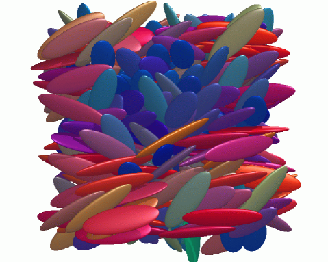
Figure 9: Snap-shot of the $1\times 3\times 10$ model in the biaxial phase (here at $p^{*}=8.0$). The ellipsoids are colour coded with respect to their orientations (colour online).

Figure 10: Plot of the equation of state for the biaxial $1\times 3\times 10$ model (isotropic: black squares, discotic: open squares, biaxial: black triangles) along with the Vega EOS for the isotropic branch.

The biaxial phase formed at $p^{*}=8.0$, however, at $p^{*}=5.0$ the system had formed a discotic phase. This indicates that the formation of a biaxial phase is a two-stage process; first orientating along the short $a$ axis, later followed by the long $c$ axis i.e. having the phase transitions isotropic - discotic - biaxial. This is in line with the observation that discotic phases form at lower volume fractions than nematic phases (the biaxial phase can be seen as being composed of both a discotic and a nematic phase).

The positions of the isotropic liquid-liquid crystal transitions found in this work are presented in Table 5. A study of the I-N transition for biaxial ellipsoids was undertaken by Tjipto-Margo and Evans Tjipto-Margo and Evans (1991) confirming the finding of Gelbart and Barboy Gelbart and Barboy (1980) that biaxiality reduces the first order nature of the I-N transition (this result was also confirmed for hard sphero-platelets by Somoza and Tarazona Somoza and Tarazona (1992)). It appears that the additional degree of freedom associated with biaxiality increases the disorder in the nematic phase with respect to a uniaxial ($D_{\infty h}$) model. At the ‘self-dual’ point (where $a:b=b:c$, i.e. $b=\sqrt{ac}$) the transition becomes second-order Mulder (1989). The isotropic-biaxial nematic transition is said to occur for models that are close to this self-dual point Allen (1990). For the uniaxial $1\times 10\times 10$ model a considerable jump can be seen in the volume fractions associated with the formation of the discotic phase (Fig. 8), one of the hall-marks of a first-order transition. Meanwhile, for the biaxial $1\times 3\times 10$ model no such jump is seen.

Table 5: Location of the isotropic-nematic transition ($S_{2}>0.4$) for hard ellipsoids (Note: $a=1$). Order parameters are given for $p^{*}=9.5$.

$b$	$c$	$p^{*}$	$y$	phase	$S_{2}(c)$	$S_{2}(a)$
prolate
1	2.5	–	–	I	$<0.1$	$<0.1$
1	4	–	–	I	$<0.1$	$<0.1$
1	5	–	–	I	0.13	$<0.1$
1	6	7.0	0.356	$N_{+}$	0.69	0.20
1	8	7.5	0.356	$N_{+}$	0.55	0.18
1	10	–	–	I	0.30	0.12
oblate
2.5	2.5	–	–	I	$<0.1$	$<0.1$
4	4	–	–	I	0.12	0.24
5	5	7.0	0.374	$N_{-}$	0.23	0.81
6	6	5.5	0.336	$N_{-}$	0.25	0.87
8	8	3.0	0.257	$N_{-}$	0.26	0.92
10	10	2.5	0.240	$N_{-}$	0.27	0.95
biaxial prolate	($b<\sqrt{ac}$)
2	5	–	–	I	0.10	$<0.1$
2	6	–	–	I	0.21	0.15
2	8	6.0	0.342	$N_{+}$	0.85	0.25
3	10	8.0	0.389	$B$	0.48	0.76
biaxial self-dual
1.25	1.5625	–	–	I	$<0.1$	$<0.1$
2	4	–	–	I	$<0.1$	$<0.1$
3	9	4.5	0.30	$N_{-}$	0.34	0.81
biaxial oblate	($b>\sqrt{ac}$)
3	6	9.0	0.402	$N_{-}$	0.23	0.46
3	8	6.0	0.338	$N_{-}$	0.27	0.78
5	8	4.5	0.313	$N_{-}$	0.25	0.90
5	10	3.5	0.269	$N_{-}$	0.30	0.92
8	10	3.0	0.249	$N_{-}$	0.27	0.95

IV Conclusions

Various ellipsoidal models have been subjected to Monte Carlo compression runs. The Vega equation of state is seen to perform very well for the isotropic phases of all of the models considered. The elongated uniaxial models show indications of the first-order nature of the isotropic-nematic transition. However, the formation of orientationally ordered phases for very long prolate models is severely hindered by the formation of a glass like state. The oblate models form discotic readily, at lower volume fractions than their prolate partners. The biaxial phase seems to form in a two-stage process, first forming a discotic phase, followed by the biaxial phase upon orientation of the long axes.

V Appendix A

Table 6: Values for $R$, $S$, $V$, $\alpha$ and $B_{2}/V$ for hard ellipsoids (Note: $a=1$).

$b$	$c$	$R$	$S$	$V$	$\alpha$	$B_{2}/V$
sphere
1	1	1	$4\pi$	$4\pi/3$	1	4
prolate
1	2.5	1.5919	26.1518	10.472	1.32516	4.97549
1	4	2.26639	40.4975	$16\pi/3$	1.82597	6.4779
1	5	2.73397	50.1925	$20\pi/3$	2.184	7.552
1	6	3.20942	59.9386	$8\pi$	2.55136	8.65409
1	8	4.17441	79.5147	$32\pi/3$	3.30174	10.9052
1	10	5.15042	99.151	$40\pi/3$	4.06377	13.1913
oblate
2.5	2.5	2.0811	50.0111	26.1799	1.32516	4.97549
4	4	3.22269	113.921	$64\pi/3$	1.82597	6.4779
5	5	3.99419	171.78	$100\pi/3$	2.184	7.552
6	6	4.76976	241.985	$48\pi$	2.55136	8.65409
8	8	6.32758	419.657	$256\pi/3$	3.30174	10.9052
10	10	7.89019	647.22	$400\pi/3$	4.06377	13.1913
biaxial
1.25	1.5625	1.28328	20.1576	8.18123	1.05395	4.16185
2	4	2.52566	63.4766	$32\pi/3$	1.59473	5.7842
2	5	2.96925	78.2743	$40\pi/3$	1.84951	6.54853
2	6	3.42527	93.1895	$16\pi$	2.11675	7.35026
2	8	4.36059	123.218	$64\pi/3$	2.67234	9.01701
3	6	3.70789	129.13	$24\pi$	2.11675	7.35026
3	8	4.60996	170.448	$32\pi$	2.60536	8.81607
3	9	5.07182	191.203	$36\pi$	2.85815	9.57446
3	10	5.53883	212.0	$40\pi$	3.11474	10.3442
5	8	5.22725	268.73	$160\pi/3$	2.7946	9.38379
5	10	6.10332	333.946	$200\pi/3$	3.24386	10.7316
8	10	7.1304	521.211	$320\pi/3$	3.69682	12.0904

In Table 6 we provide a table of $R$, $S$, $V$, $\alpha$ and $B_{2}/V$ for the various models studied in this work. The values for $R$ and $S$ are obtained by evaluating the expressions derived by Singh and Kumar Singh and Kumar (1996, 2001). Thus the mean radius of curvature is given by

$$R=\frac{a}{2}\left[\sqrt{\frac{1+\epsilon_{b}}{1+\epsilon_{c}}}+\sqrt{\epsilon}_{c}\left\{\frac{1}{\epsilon_{c}}F(\varphi,k_{1})+E(\varphi,k_{1})\right\}\right],$$ (11)

and the surface area by

$$S=2\pi a^{2}\left[1+\sqrt{\epsilon_{c}(1+\epsilon_{b})}\left\{\frac{1}{\epsilon_{c}}F(\varphi,k_{2})+E(\varphi,k_{2})\right\}\right],$$ (12)

where $F(\varphi,k)$ is an elliptic integral of the first kind and $E(\varphi,k)$ is an elliptic integral of the second kind, with the amplitude being

$$\varphi=\tan^{-1}(\sqrt{\epsilon}_{c}),$$ (13)

and the moduli

$$k_{1}=\sqrt{\frac{\epsilon_{c}-\epsilon_{b}}{\epsilon_{c}}},$$ (14)

and

$$k_{2}=\sqrt{\frac{\epsilon_{b}(1+\epsilon_{c})}{\epsilon_{c}(1+\epsilon_{b})}},$$ (15)

where the anisotropy parameters, $\epsilon_{b}$ and $\epsilon_{c}$, are

$$\epsilon_{b}=\left(\frac{b}{a}\right)^{2}-1,$$ (16)

and

$$\epsilon_{c}=\left(\frac{c}{a}\right)^{2}-1.$$ (17)

The volume of the ellipsoid is given by the well known

$$V=\frac{4\pi}{3}abc.$$ (18)

Note the symmetry between the prolate and oblate ellipsoids for the values of $\alpha$, and thus for $B_{2}$.

References

- Metropolis et al. (1953) N. Metropolis, A. W. Rosenbluth, M. N. Rosenbluth, A. H. Teller, and E. Teller, J. Chem. Phys. 21, 1087 (1953).
- Alder and Wainwright (1957) B. J. Alder and T. E. Wainwright, J. Chem. Phys. 27, 1208 (1957).
- Wood (1963) W. W. Wood, Los Alamos Scientific Laboratory Report LA-2827 (1963).
- Wood (1970) W. W. Wood, J. Chem. Phys. 52, 729 (1970).
- Vieillard-Baron (1972) J. Vieillard-Baron, J. Chem. Phys. 56, 4729 (1972).
- Cuesta and Frenkel (1990) J. A. Cuesta and D. Frenkel, Phys. Rev. A 42, 2126 (1990).
- Frenkel et al. (1984) D. Frenkel, B. M. Mulder, and J. P. McTague, Phys. Rev. Lett. 52, 287 (1984).
- Evans (2002) B. Evans, Molec. Phys. 100, 199 (2002).
- Frenkel and Mulder (1985) D. Frenkel and B. M. Mulder, Molec. Phys. 55, 1171 (1985).
- Mulder and Frenkel (1985) B. Mulder and D. Frenkel, Molec. Phys. 55, 1193 (1985).
- Freiser (1970) M. J. Freiser, Phys. Rev. Lett. 24, 1041 (1970).
- Madsen et al. (2004) L. A. Madsen, T. J. Dingemans, M. Nakata, and E. T. Samulski, Phys. Rev. Lett. 92, 145505 (2004).
- Acharya et al. (2004) B. R. Acharya, A. Primak, and S. Kumar, Phys. Rev. Lett. 92, 145506 (2004).
- Perram and Praestgaard (1988) J. W. Perram and E. Praestgaard, Molec. Phys. 63, 1103 (1988).
- McBride and Vega (2002) C. McBride and C. Vega, J. Chem. Phys. 117, 10370 (2002).
- Wu and Sadus (2002) G.-W. Wu and R. J. Sadus, Fluid Phase Equilib. 194, 227 (2002).
- Murat and Kantor (2006) M. Murat and Y. Kantor, Phys. Rev. E 74, 031124 (2006).
- Michele et al. (2006) C. D. Michele, A. Scala, R. Schilling, and F. Sciortino, J. Chem. Phys. 124, 104509 (2006).
- Donev et al. (2004a) A. Donev, I. Cisse, D. Sachs, E. A. Variano, F. H. Stillinger, R. Connelly, S. Torquato, and P. M. Chaikin, Science 303, 990 (2004a).
- Donev et al. (2004b) A. Donev, F. H. Stillinger, P. M. Chaikin, and S. Torquato, Phys. Rev. Lett. 92, 255506 (2004b).
- Donev et al. (2005) A. Donev, S. Torquato, and F. H. Stillinger, J. Comput. Phys. 202, 737 (2005).
- Doneva et al. (2005) A. Doneva, S. Torquatoa, and F. H. Stillinger, J. Comput. Phys. 202, 765 (2005).
- Basavaraj et al. (2006) M. G. Basavaraj, G. G. Fuller, J. Fransaer, and J. Vermant, Langmuir 22, 6605 (2006).
- Man et al. (2005) W. Man, A. Donev, F. H. Stillinger, M. T. Sullivan, W. B. Russel, D. Heeger, S. Inati, S. Torquato, and P. M. Chaikin, Phys. Rev. Lett. 94, 198001 (2005).
- Allen (1990) M. P. Allen, Liq. Cryst. 8, 499 (1990).
- Camp and Allen (1997) P. J. Camp and M. P. Allen, J. Chem. Phys. 106, 6681 (1997).
- Wang et al. (2001) W. Wang, J. Wang, and M.-S. Kim, Computer Aided Geometric Design 18, 531 (2001).
- Perram and Wertheim (1985) J. W. Perram and M. S. Wertheim, J. Comput. Phys. 58, 409 (1985).
- Straley (1974) J. P. Straley, Phys. Rev. A 10, 1881 (1974).
- Eppenga and Frenkel (1984) R. Eppenga and D. Frenkel, Molec. Phys. 52, 1303 (1984).
- Zannoni (1979) C. Zannoni, in The Molecular physics of liquid crystals, edited by G. R. Luckhurst and G. W. Gray (Academic Press, 1979), chap. 3, p. 51.
- Boublik and Nezbeda (1986) T. Boublik and I. Nezbeda, Coll. Czech. Chem. Commun. 51, 2301 (1986).
- Isihara (1950) A. Isihara, J. Chem. Phys. 18, 1446 (1950).
- Isihara and Hayashida (1951a) A. Isihara and T. Hayashida, J. Phys. Soc. Jpn. 6, 40 (1951a).
- Isihara and Hayashida (1951b) A. Isihara and T. Hayashida, J. Phys. Soc. Jpn. 6, 46 (1951b).
- Nezbeda (1976) I. Nezbeda, Chem. Phys. Lett. 41, 55 (1976).
- Parsons (1979) J. D. Parsons, Phys. Rev. A 19, 1225 (1979).
- Song and Mason (1990) Y. Song and E. A. Mason, Phys. Rev. A 41, 3121 (1990).
- Rigby (1989) M. Rigby, Molec. Phys. 66, 1261 (1989).
- Wertheim (2001) M. S. Wertheim, Molec. Phys. 99, 187 (2001).
- Maeso and Solana (1993) M. Maeso and J. Solana, Molec. Phys. 79, 1365 (1993).
- Vega (1997) C. Vega, Molec. Phys. 92, 651 (1997).
- Onsager (1949) L. Onsager, Ann. (N.Y.) Acad. Sci. 51, 627 (1949).
- Isihara (1951) A. Isihara, J. Chem. Phys. 19, 1142 (1951).
- Zarragoico chea et al. (1992) G. Zarragoico chea, D. Levesque, and J. Weis, Molec. Phys. 75, 989 (1992).
- Allen and Mason (1995) M. P. Allen and C. P. Mason, Molec. Phys. 86, 467 (1995).
- Vega et al. (2001) C. Vega, C. McBride, and L. G. MacDowell, J. Chem. Phys. 115, 4203 (2001).
- Samborski et al. (1994) A. Samborski, G. T. Evans, C. P. Mason, and M. Allen, Molec. Phys. 81, 263 (1994).
- Tjipto-Margo and Evans (1991) B. Tjipto-Margo and G. T. Evans, J. Chem. Phys. 94, 4546 (1991).
- Gelbart and Barboy (1980) W. M. Gelbart and B. Barboy, Accounts of Chemical Research 13, 290 (1980).
- Somoza and Tarazona (1992) A. M. Somoza and P. Tarazona, Molec. Phys. 75, 17 (1992).
- Mulder (1989) B. Mulder, Phys. Rev. A 39, 360 (1989).
- Singh and Kumar (1996) G. S. Singh and B. Kumar, J. Chem. Phys. 105, 2429 (1996).
- Singh and Kumar (2001) G. S. Singh and B. Kumar, Annals of Physics 294, 24 (2001).