Moment equations in a Lotka-Volterra extended system with time correlated noise

Abstract

A spatially extended Lotka-Volterra system of two competing species in the presence of two correlated noise sources is analyzed: (i) an external multiplicative time correlated noise, which mimics the interaction between the system and the environment; (ii) a dichotomous stochastic process, whose jump rate is a periodic function, which represents the interaction parameter between the species. The moment equations for the species densities are derived in Gaussian approximation, using a mean field approach. Within this formalism we study the effect of the external time correlated noise on the ecosystem dynamics. We find that the time behavior of the $1^{st}$ order moments are independent on the multiplicative noise source. However the behavior of the $2^{nd}$ order moments is strongly affected both by the intensity and the correlation time of the multiplicative noise. Finally we compare our results with those obtained studying the system dynamics by a coupled map lattice model.

05.10.-a, 05.40.-a, 87.23.Cc

1 Introduction

Real ecosystems are influenced by the presence of continuous external fluctuations connected to the random variation of environmental parameters such as temperature and natural resources, which affects the system dynamics by a multiplicative nonlinear interaction [1]. The spatio-temporal behaviour and the formation of spatial patterns became recently an important topic in hydrodynamics systems, nonlinear optics, oscillatory chemical reactions and in theoretical ecology [2]-[4]. During the last three decades a new approach, based on the use of moments, has been exploited to describe the behaviour of spatially extended system in population dynamics, quantum systems in the context of nonlinear Schrödinger equations, and kinetic models of polymer dynamics [5]-[7]. In this paper, by using the formalism of the moments, we study the spatio-temporal behaviour of a two-dimensional system formed by two competing species subject to random fluctuations. The system is described by generalized Lotka-Volterra equations in the presence of two noise sources: (i) a multiplicative time correlated noise with correlation times $\tau^{c}$, modeled as an Ornstein-Uhlenbeck process [8], which takes the environment fluctuations acting on the species into account; (ii) a noisy interaction parameter which is a stochastic process, whose dynamics is given by a periodic function in the presence of a correlated dichotomous noise, with correlation time $\tau_{d}$. We define a two-dimensional spatial domain considering in each site a system of two Lotka-Volterra equations coupled by an interaction term [9]. Afterwards, using a mean field approach, we study the dynamics of the system by the moment equations, within the Gaussian approximation [10, 11], getting the time behavior of the $1^{st}$ and $2^{nd}$ order moments of the species concentrations. Finally we compare our results with those obtained within the formalism of the coupled map lattice (CML) model [12].

2 The model

Our system is described by a time evolution model of Lotka-Volterra equations, within the Ito scheme [13]-[15], with diffusive terms in a spatial lattice with $N$ sites

$$\dot{x}_{i,j} = \mu x_{i,j}(1-x_{i,j}-\beta y_{i,j})+x_{i,j}\sqrt{\sigma_{x}}\zeta^{x}_{i,j}+D\sum_{\gamma}(x_{\gamma}-x_{i,j})$$ (1)

$$\dot{y}_{i,j} = \mu y_{i,j}(1-y_{i,j}-\beta x_{i,j})+y_{i,j}\sqrt{\sigma_{y}}\zeta^{y}_{i,j}+D\sum_{\gamma}(y_{\gamma}-y_{i,j}),$$ (2)

where $x_{i,j}$ and $y_{i,j}$ denote respectively the densities of species $x$ and species $y$ in the lattice site $(i,j)$, $\mu$ is the growth rate, $D$ is the diffusion constant, and $\sum_{\gamma}$ indicates the sum over all the sites except the pair $(i,j)$. Here $\beta$ is the interaction parameter. $\zeta^{l}(t)$ $(l=x,y)$ are statistically independent colored noises, i. e. exponentially correlated processes given by the Ornstein-Uhlenbeck process [8]

$$\frac{d\zeta^{l}}{dt}=-\frac{1}{\tau^{c}_{l}}\zeta^{l}+\frac{1}{\tau^{c}_{l}}\xi^{l}(t)\qquad(l=x,y)$$ (3)

and $\xi^{l}(t)$ $(l=x,y)$ are Gaussian white noises within the Ito scheme with zero mean and correlation function $\langle\xi^{l}(t)\xi^{m}(t^{\prime})\rangle=2\sigma\delta(t-t^{\prime})\delta_{lm}$. The correlation function of the processes of Eq.(3) is

$$\langle\zeta^{l}(t)\zeta^{m}(t^{\prime})\rangle=\frac{\sigma}{\tau^{c}_{l}}e^{-|t-t^{\prime}|/\tau^{c}_{l}}\delta_{lm}$$ (4)

and gives $2\delta(t-t^{\prime})\delta_{lm}$ in the limit $\tau^{c}_{l}\rightarrow 0$.

2.1 The interaction parameter

The value of the interaction parameter $\beta$ is crucial for the dynamical regime of the ecosystem investigated. In fact, for $\beta<1$ both species survive and a coexistence regime takes place, while for $\beta>1$ one of the two species extinguishes after a certain time and exclusion occurs. These two regimes correspond to stable states of the Lotka-Volterra’s deterministic model [13]. Moreover periodical and random driving forces connected with environmental and climatic variables, such as the temperature, modify the dynamics of the ecosystem, affecting both directly the species densities and the interaction parameter. This causes the system dynamics to change between coexistence ($\beta<1$) and exclusion ($\beta>1$) regimes. To describe this dynamical behavior we consider as interaction parameter $\beta(t)$ a dichotomous stochastic process, whose jump rate is a periodic function

$$\gamma(t) = 0,\qquad\qquad\qquad\qquad\enspace\Delta t\leq\tau_{d}$$

$$\gamma(t) = \gamma_{0}\left(1+A\thinspace|\cos\omega t|\right),\quad\Delta t>\tau_{d}\;.$$

Here $\Delta t$ is the time interval between two consecutive switches, and $\tau_{d}$ is the delay between two jumps, that is the time interval after a switch, before another jump can occur. In Eq. (LABEL:jump_rate), $A$ and $\omega=(2\pi)/T$ are respectively the amplitude and the angular frequency of the periodic term, and $\gamma_{0}$ is the jump rate in the absence of periodic term. Setting $\beta_{down}=0.94<1$ and $\beta_{up}=1.04>1$, the dichotomous noise causes $\beta(t)$ to jump between two values, $\beta_{down}$ and $\beta_{up}$. The value $\tau_{d}=43.5$ for the delay corresponds to a competition regime with $\beta$ switching quasi-periodically from coexistence to exclusion regimes [11] (see Fig. 1).

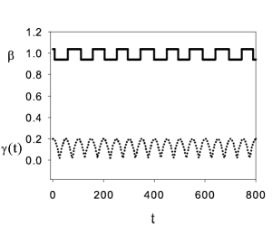
Figure 1: Time evolution of the interaction parameter $\beta(t)$, driven by time correlated dichotomous noise with correlation time $\tau_{d}=43.5$. $\beta(t)$ jumps between $\beta_{down}=0.94$ and $\beta_{up}=1.04$. The initial value is $\beta(0)=\beta_{up}=1.04$. The values of the other parameters are: $A=9.0$, $\omega/(2\pi)=10^{-2}$, $\gamma_{0}=2\cdot 10^{-2}$.

This synchronization phenomenon is due to the choice of the $\tau_{d}$ value, which stabilizes the jumps in such a way they happen for high values of the jump rate, that is for values around the maximum of the function $\gamma(t)$. This causes a quasi-periodical time behaviour of the species concentrations $x$ and $y$, which can be considered as a signature of the stochastic resonance phenomenon [14].

3 Mean field model

In this section we derive the moment equations for our system. Assuming $N\rightarrow\infty$, we write Eqs. (1) and (2) in mean field form

$$\dot{x} = f_{x}(x,y)+\sqrt{\sigma_{x}}g_{x}(x)\zeta^{x}+D(<x>-x)$$ (6)

$$\dot{y} = f_{y}(x,y)+\sqrt{\sigma_{y}}g_{y}(y)\zeta^{y}+D(<y>-y),$$ (7)

where $<x>$ and $<y>$ are average values on the spatial lattice considered, that is the ensemble average in the thermodynamics limit. We set $f_{x}(x,y)=\mu x(1-x-\beta y)$, $g_{x}(x)=x$, $f_{y}(x,y)=\mu y(1-y-\beta x)$, $g_{y}(y)=y$. By site averaging Eqs. (6) and (7), we obtain

$$<\dot{x}>~{}=~{}<f_{x}(x,y)>,$$ (8)

$$<\dot{y}>~{}=~{}<f_{y}(x,y)>.$$ (9)

By expanding the functions $f_{x}(x,y)$, $g_{x}(x)$, $f_{y}(x,y)$, $g_{y}(y)$ around the $1^{st}$ order moments $<x>$ and $<y>$, we get an infinite set of simultaneous ordinary differential equations for all the moments. This equation set is truncated by using a Gaussian approximation, which causes the cumulants above the $2^{nd}$ order to vanish. Therefore we obtain

$$<\dot{x}> = \mu<x>(1-<x>-\beta<y>)-\mu(\beta\mu_{11}+\mu_{20})$$ (10)

$$<\dot{y}> = \mu<y>(1-<y>-\beta<x>)-\mu(\beta\mu_{11}+\mu_{02})$$ (11)

$$\dot{\mu}_{20} = 2\mu\mu_{20}-2D\mu_{20}-2\mu\beta<y>\mu_{20}-2\mu<x>(\beta\mu_{11}+2\mu_{20})$$ (12)

$$+ 2\sigma_{x}(<x>^{2}+\mu_{20})(1-e^{-\frac{t}{\tau_{x}^{c}}})$$

$$\dot{\mu}_{02} = 2\mu\mu_{02}-2D\mu_{02}-2\mu\beta<x>\mu_{02}-2\mu<y>(\beta\mu_{11}+2\mu_{02})$$ (13)

$$+ 2\sigma_{y}(<y>^{2}+\mu_{02})(1-e^{-\frac{t}{\tau_{y}^{c}}})$$

$$\dot{\mu}_{11} = 2\mu\mu_{11}-2D\mu_{11}-<x>[2\mu\mu_{11}+\mu\beta(\mu_{11}+\mu_{02})]$$ (14)

$$- <y>[2\mu\mu_{11}+\mu\beta(\mu_{11}+\mu_{20})]~{},$$

where $\mu_{20}$, $\mu_{02}$, $\mu_{11}$ are the $2^{nd}$ order central moments defined on the lattice

$$\mu_{20} = <x^{2}>-<x>^{2},\qquad\mu_{02}=<y^{2}>-<y>^{2},$$ (15)

$$\mu_{11} = <xy>-<x><y>~{}.$$ (16)

The dynamics of the two species is analyzed through the time behavior of $1^{st}$ and $2^{nd}$ order moments according to Eqs. (10)-(14), for different values both of intensities $\sigma$ ($=\sigma_{x}=\sigma_{y}$) and correlation time $\tau^{c}$ (=$\tau_{x}^{c}=\tau_{y}^{c}$) of the multiplicative colored noise. The results are reported in Figs. 2-4. The results shown in Fig. 2, obtained with a low value of the correlation time $\tau^{c}$ reproduce the same time behavior obtained for uncorrelated white noise sources in Ref. [11]. The value of the time delay is $\tau_{d}=43.5$, which determines a quasi-periodic switching between the coexistence and exclusion regimes. The values of the other parameters are: $\mu=2$, $D=0.05$. The initial conditions are: $\zeta^{x}(0)=\zeta^{y}(0)=0$, $<x(0)>$ = $<y(0)>$ = $0.1$, $\mu_{20}(0)=\mu_{02}(0)=\mu_{11}(0)=0$. These initial values for the moments correspond to uniformly distributed species on the considered lattice. In Figs. 2a, 3a, 4a we note that the $1^{st}$ order moments undergo correlated oscillations around $0.5$. This behaviour is independent both on the intensity and the correlation time of the multiplicative noise. On the other hand the behavior of the $2^{nd}$ order moments depends strongly both on the intensity and the correlation time of the external multiplicative noise. In the absence of noise $\mu_{20}$, $\mu_{02}$, $\mu_{11}$ maintain their initial values. For very low levels of multiplicative noise ($\sigma=10^{-12}$) quasi-periodical oscillations appear with the same frequency of the interaction parameter $\beta(t)$, because the noise breaks the symmetry of the dynamical behavior of the $2^{nd}$ order moments (see Figs. 2b, 3b, 4b). About the variances of the two species, the time series of $\mu_{20}$ and $\mu_{02}$, which coincide all the time, show an oscillating behaviour characterized by small (close to zero) and large values. However the negative values of the correlation $\mu_{11}$ indicate that the two species distributions are anticorrelated. In particular, we find a time behavior characterized by anticorrelated oscillations, whose amplitude increases with the multiplicative noise intensity and it is reduced as the correlation time becomes bigger (see Figs. 2b, 3b, 4b).

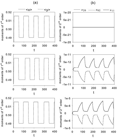
Figure 2: Time evolution of the $1^{st}$ and $2^{nd}$ order moments for $\tau^{c}=1$. The time series of (a) $<x(t)>$ and $<y(t)>$, and (b) $\mu_{2,0}$ and $\mu_{0,2}$ respectively, are completely overlapped. The values of the multiplicative noise intensity are: $\sigma=0,10^{-12},10^{-6}$, from top to bottom. Here $\tau_{d}=43.5$, $\mu=2$, and $D=0.05$. The initial conditions are: $\zeta^{x}(0)=\zeta^{y}(0)=0$, $<x(0)>$ = $<y(0)>$ = $0.1$, $\mu_{20}(0)=\mu_{02}(0)=\mu_{11}(0)=0$. The values of the other parameters are the same of Fig. 1.

Figure 3: Time evolution of the $1^{st}$ and $2^{nd}$ order moments for $\tau^{c}=10$. Here (a) $<x(t)>$ and $<y(t)>$, and (b) $\mu_{2,0}$ and $\mu_{0,2}$ respectively, are overlapped. The values of the multiplicative noise intensity are: $\sigma=10^{-12},10^{-6}$, from top to bottom. The values of the other parameters and the initial conditions are the same of Fig. 2.

Figure 4: Time evolution of the $1^{st}$ and $2^{nd}$ order moments for $\tau^{c}=100$. Here (a) $<x(t)>$ and $<y(t)>$, and (b) $\mu_{2,0}$ and $\mu_{0,2}$ respectively, are overlapped. The values of the multiplicative noise intensity are: $\sigma=10^{-12},10^{-6}$, from top to bottom. The values of the other parameters and the initial conditions are the same of Fig. 2.

This anticorrelated behaviour indicates that the spatial distribution in the lattice will be characterized by zones with a maximum of concentration of species $x$ and a minimum of concentration of species $y$ and viceversa. The two species will be distributed therefore in non-overlapping spatial patterns. This physical picture is in agreement with previous results obtained with a different model [15]. A further increase of the multiplicative noise intensity ($\sigma=10^{-6}$) causes an enhancement of the oscillation amplitude both in $\mu_{20}$, $\mu_{02}$ and $\mu_{11}$. This gives information on the probability density of both species, whose width and mean value undergo the same oscillating behavior. The anticorrelated behavior is enhanced by increasing the noise intensity value. We note that the amplitude of the oscillations is of the same order of magnitude of the noise intensity $\sigma$, that is the amplitude of the oscillations is enhanced as the noise intensity increases. The periodicity of these noise-induced oscillations shown in Figs. 2-4 is the same of the interaction parameter $\beta(t)$ (see Fig. 1). Moreover the right-hand side of Figs. 2-4 shows that the multiplicative colored noise affects the time evolution of the $2^{nd}$ order moments introducing a delay: the amplitude of the oscillations reaches its highest value after a time interval whose length increases as $\tau^{c}$ becomes bigger. In fact by comparing the first figures in Figs. 2b-4b with $\sigma=10^{-12}$, for example, the maximum is reached approximately at $t\simeq 110$ for $\tau^{c}=1$, and at $t\simeq 330$ for $\tau^{c}=100$.

4 Coupled Map Lattice Model

Our results, obtained by using moment equations in Gaussian approximation, can be checked studying the dynamics of the system by a different approach, namely the CML model

$$x_{i,j}^{(n+1)} = \mu x_{i,j}^{(n)}(1-x_{i,j}^{(n)}-\beta^{(n)}y_{i,j}^{(n)})+\sqrt{\sigma_{x}}x_{i,j}^{(n)}\zeta_{i,j}^{x{(n)}}+D\sum_{\gamma}(x_{\gamma}^{(n)}-x_{i,j}^{(n)})\enspace\qquad$$ (17)

$$y_{i,j}^{(n+1)} = \mu y_{i,j}^{(n)}(1-y_{i,j}^{(n)}-\beta^{(n)}x_{i,j}^{(n)})+\sqrt{\sigma_{y}}y_{i,j}^{(n)}\zeta_{i,j}^{y{(n)}}+D\sum_{\gamma}(y_{\gamma}^{(n)}-y_{i,j}^{(n)}),\enspace\qquad$$ (18)

which represents a discrete version of the Lotka-Volterra equations.

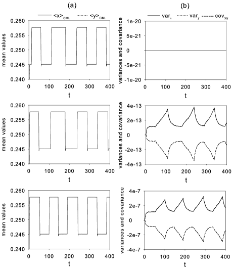
Figure 5: (a) Mean values: $<x>_{{}_{CML}}$, $<y>_{{}_{CML}}$, and (b) variances: $var_{x}$, $var_{y}$ and $cov_{xy}$ of the two species, as a function of time for $\tau^{c}=1$. The values of the multiplicative noise intensity are: $\sigma=0,10^{-12},10^{-6}$, from top to bottom. The initial values of the species concentrations are $x_{i,j}^{(0)}=y_{i,j}^{(0)}=0.1$ for all sites $(i,j)$. The values of the other parameters are the same of Fig. 2.

Figure 6: (a) Mean values: $<x>_{{}_{CML}}$, $<y>_{{}_{CML}}$, and (b) variances: $var_{x}$, $var_{y}$ and $cov_{xy}$ of the two species, as a function of time for $\tau^{c}=10$. The values of the multiplicative noise intensity are: $\sigma=10^{-12},10^{-6}$, from top to bottom. The values of the other parameters and the initial conditions are the same of Fig. 5.

Figure 7: (a) Mean values: $<x>_{{}_{CML}}$, $<y>_{{}_{CML}}$, and (b) variances: $var_{x}$, $var_{y}$ and $cov_{xy}$ of the two species, as a function of time for $\tau^{c}=100$. The values of the multiplicative noise intensity are: $\sigma=10^{-12},10^{-6}$, from top to bottom. The values of the other parameters and the initial conditions are the same of Fig. 5.

Here $x^{(n)}_{i,j}$ and $y^{(n)}_{i,j}$ denote respectively the densities of preys $x$ and $y$ in the site $(i,j)$ at the time step $n$, $\mu$ is the growth rate and $D$ is the diffusion constant. The interaction parameter $\beta^{(n)}$ corresponds to the value of $\beta(t)$ taken at the time step $n$, according to Eq. (LABEL:jump_rate). $\zeta_{i,j}^{x(n)}$ and $\zeta_{i,j}^{y(n)}$ are independent Gaussian colored noise sources above defined in Eq. (3). Finally $\sum_{\gamma}$ indicates the sum over the four nearest neighbors. To evaluate the $1^{st}$ and $2^{nd}$ order moments we define on the lattice, at the time step $n$, the mean values $<x>_{{}_{CML}}^{(n)}$, $<y>_{{}_{CML}}^{(n)}$,

$$<z>_{{}_{CML}}^{(n)}~{}=~{}\frac{\sum_{i,j}z^{(n)}_{i,j}}{N}~{},\qquad z=x,y$$ (19)

the standard deviations $var^{(n)}_{x}$, $var^{(n)}_{y}$

$$var^{(n)}_{z}=\sqrt{\frac{\sum_{i,j}(z^{(n)}_{i,j}-<z>^{(n)})^{2}}{N}}~{},\qquad z=x,y$$ (20)

and the covariance $cov^{(n)}_{xy}$ of the two species

$$cov^{(n)}_{xy}=\frac{\sum_{i,j}(x^{(n)}_{i,j}-<x>^{(n)})(y^{(n)}_{i,j}-<y>^{(n)})}{N},$$ (21)

where $N=100\times 100$ is the number of lattice sites. We note that $<x>_{{}_{CML}}$, $<y>_{{}_{CML}}$ and $var_{x}$, $var_{y}$, $cov_{xy}$, corresponding respectively to $<x>$, $<y>$, and $\mu_{20}$, $\mu_{02}$, $\mu_{11}$ obtained within the mean field approach, are the $1^{st}$ and $2^{nd}$ order moments defined within the scheme of the CML model. The time behavior of these quantities, for three different values of the multiplicative noise intensity, and for three different values of the correlation time is reported in Figs. 5-7. Comparing these results with those shown in Figs. 2-4, we note that the time behaviour obtained for the $1^{st}$ and $2^{nd}$ order moments by the CML model is in a good qualitative agreement with those found using the mean field approach. In particular we note the role played by the multiplicative noise: higher noise intensity causes the $2^{nd}$ order moments to increase (see in Figs. 5-7 the enhancement of the oscillation maxima as the multiplicative noise intensity increases). This indicates both a spread of the two species concentrations and a spatial anticorrelation between them. These results agree with those found within the formalism of the moment equations. We observe that the time behaviour of $var_{x}$, $var_{y}$, $cov_{xy}$ is characterized by the presence of oscillations whose maximum amplitude is reached after a time delay. This peculiarity is the same of that found within the mean field approach (see paragraph $3$). The discrepancies in the oscillation intensities are due to: (i) the Gaussian approximation in the moment formalism; (ii) the fact that the species interaction in the CML model is restricted to the nearest neighbors; (iii) the different stationary values of the species densities in the considered models. Specifically, using for $\beta$ an average value, $\beta_{aver}=(\beta_{up}+\beta_{down})/2$, we get: $x_{st}=y_{st}=1/(1+\beta_{aver})\simeq 0.5$ for the mean field model, and $x_{st}^{{}^{CML}}=y_{st}^{{}^{CML}}=(1-1/\mu)/(1+\beta_{aver})\simeq 0.25$ for the CML model.

5 Conclusions

By using the moment formalism in Gaussian approximation, we describe the time behavior of two competing species inside a two-dimensional spatial domain in the presence both of a multiplicative colored noise and a dichotomous noise. We find that the $1^{st}$ order moments of the two species densities show correlated oscillations, whose amplitude is independent on the multiplicative noise. However, the behavior of the $2^{nd}$ order central moments depend strongly both on the intensity $\sigma$ and the correlation time $\tau^{c}$ of the multiplicative noise. In particular, the behavior of the $2^{nd}$ order mixed moment $\mu_{11}$ indicates that higher values of the multiplicative noise intensity push the two species towards an anticorrelated regime characterized by oscillations whose maximum amplitude is reached after a delay time: this delayed behaviour depends on the correlation time $\tau^{c}$. We find a good qualitative agreement between these results, obtained within the mean field approach, and those found by the CML model. In view of some applications of our model, to describe and to predict the behaviour of biological species, we note that in real ecosystems the fluctuations are characterized by a cut-off. Therefore experimental data [16], whose dynamics is strongly affected by noisy perturbations and stochastic environmental variables, can be better modeled using sources of colored noise.

6 Acknowledgments

This work was supported by ESF (European Science Foundation) STOCHDYN network, MIUR, INFM-CNR and CNISM.

References

- [1] Special section on Complex Systems, Science 284, 79 (1999); O. N. Bjornstad and B. T. Grenfell, Science 293, 638 (2001); S. Ciuchi, F. de Pasquale and B. Spagnolo, Phys. Rev. E 53, 706 (1996); M. Scheffer, S. Carpenter, J. A. Foley, C. Folke, B. Walker, Nature 413, 591 (2001).
- [2] M. C. Cross, P. C. Hohenberg, Rev. Mod. Phys. 65, 851 (1993).
- [3] M. Kowalik, A. Lipowski, A. L. Ferreira, Phys. Rev. E 66, 066107 (2002); J. Buceta and K. Lindenberg, Phys. Rev. E 66, 046202 (2002); R. V. Solé, J. Valls, Phys. Lett. A 166, 123 (1992).
- [4] A. R. E. Sinclair, S. Mduma and J. S. Brashares, Nature 425, 288 (2003).
- [5] B. Bolker, and S. W. Pacala, Theor. Popul. Biol. 52, 179 (1997); A. Gandhi, S. Levin, S. Orszag, Bull. Math. Biol. 62, 595 (2000); J. Dushoff, Theor. Popul. Biol. 56, 325 (1999).
- [6] V. M. Peréz García, P. Torres, and G. D. Montesinos, nlin.PS/0510044 (2005).
- [7] P. Ilg, I. V. Karlin, and H. C. Öttinger, Phys. Rev. E 60, 5783 (1999).
- [8] C. W. Gardiner Handbook of stochastic methods for physics, chemistry and the natural sciences, Springer, Berlin, 1993.
- [9] A. J. Lotka, Proc. Nat. Acad. Sci. U.S.A. 6, 410 (1920); V. Volterra, Nature 118, 558 (1926).
- [10] R. Kawai, X. Sailer, L. Schimansky-Geier, C. Van den Broeck, Phys. Rev. E 69, 051104 (2004).
- [11] D. Valenti, L. Schimansky-Geier, X. Sailer and B. Spagnolo, Eur. Phys. J. B 50, 199 (2006).
- [12] K. Kaneko, Chaos 2, 279 (1992); R. V. Solé, J. Bascompte, J. Valls, Chaos 2, 387 (1992); R. V. Solé, J. Bascompte, J. Valls, J. Theor. Biol. 159, 469 (1992).
- [13] D. Valenti, A. Fiasconaro and B. Spagnolo, Physica A 331, 477 (2004); Mod. Prob. Stat. Phys. 2, 91 (2003); J. M. G. Vilar and R. V. Solé, Phys. Rev. Lett. 80, 4099 (1998).
- [14] R. Benzi, A. Sutera, A. Vulpiani, J. Phys.: Math Gen. 14, L453 (1981); L. Gammaitoni, P. Hanggi, P. Jung, and F. Marchesoni, Rev. Mod. Phys. 70, 223 (1998).
- [15] D. Valenti, A. Fiasconaro and B. Spagnolo, Fluc. Noise Lett. 5, L337 (2005).
- [16] J. García Lafuente, A. García, S. Mazzola, L. Quintanilla, J. Delgado, A. Cuttitta and B. Patti, Fishery Oceanography 11, 31 (2002); A. Caruso, M. Sprovieri, A. Bonanno, R. Sprovieri, Riv. Ital. Paleont. Strat. 108, 297 (2002).