On the nature and dynamics of low-energy cavity polaritons

Abstract

Low-energy polaritons in semiconductor microcavities are important for many processes such as, e.g., polariton condensation. Organic microcavities frequently feature both strong exciton-photon coupling and substantial scattering in the exciton subsystem. Low-energy polaritons possessing small or vanishing group velocities are especially susceptible to the effects of such scattering that can render them strongly localized. We compare the time evolution of low-energy wave packets in perfect microcavities and in a model 1$d$ cavity with diagonal disorder to illustrate this localization of polaritons and to draw attention to the need to explore its consequences for the kinetics and collective properties of polaritons.

I Introduction

Planar semiconductor microcavities have attracted much attention as they provide a method to enhance and control the interaction between the light and electronic excitations. When the microcavity mode (cavity photon) is resonant with the excitonic transition, two different regimes can be distinguished based on the competition between the processes of the exciton-photon coupling and damping (both photon damping and exciton dephasing). The weak coupling regime corresponds to the damping prevailing over the light-matter interaction, and the latter then simply modifies the radiative decay rate and the emission angular pattern of the cavity mode. In contrast, in the strong coupling regime the damping processes are weak in comparison with the exciton-photon interaction, and the true eigenstates of the system are mixed exciton-photon states, cavity polaritons. This particularly results in the appearance of the gap in the spectrum of the excitations whose magnitude is established by Rabi (splitting) energy. In inorganic semiconductors the strong coupling regime has been investigated extensively, both experimentally and theoretically,Burstein and Weisbuch (1995); Weisbuch and Rarity (1996); Skolnick et al. (1998); Khitrova et al. (1999); Kavokin and Malpuech (2003); Bassani (2003); Weisbuch and Benisty (2005) and the dynamics of microcavity polaritons is now reasonably well understood.Tassone et al. (1997) These studies continue to expand because of the prospect of important applications such as the polariton laser related to the polariton condensation in the lowest energy state.Imamoglu et al. (1996); Yamamoto (2000); Savvidis et al. (2000a); Stevenson et al. (2000); Savvidis et al. (2000b); Alexandrou et al. (2001); Deng et al. (2002); Kavokin and Malpuech (2003); Rubo et al. (2003); Laussy et al. (2004)

In another development, organic materials have been utilized in microcavities as optically active semiconductors. In many organic materials excitons are known to be small-radius states, Frenkel excitons, which interact much stronger with photons than large-radius Wannier-Mott excitons in inorganic semiconductors. The cavity polaritons, therefore, may exhibit much larger Rabi splittings on the order of few hundreds of meV; large splittings have in fact been observed experimentally.Lidzey et al. (1998, 1999); Tartakovskii et al. (2001); Hobson et al. (2002); Schouwink et al. (2002); Lidzey et al. (2002); Takada et al. (2003); Lidzey (2002, 2003); Holmes and Forrest (2004, 2005) At the same time, Frenkel excitons typically also feature substantially stronger interactions with phonons and disorder - electronic resonances in both disordered and crystalline organic systems are frequently found rather broad and dispersionless. It is thus likely that manifestations of exciton-polaritons in organic microcavities could be quite different from the corresponding inorganic counterparts.

In this paper we are concerned with the nature and dynamics of the low energy exciton-polaritons in organic microcavities, the states of particular importance for the problem of polariton condensation. Our goal here is to illustrate some qualitative features of the dynamics in both perfect and disordered systems and, thereby, to draw attention to the need of more detailed experimental and theoretical studies to elucidate conditions for the polariton laser operation based on organic systems.

The bare planar cavity photons are coherent wave excitations with a continuous spectrum and whose energy $\epsilon(\mathbf{k})=\epsilon_{k}$ depends on the magnitude $k=|\mathbf{k}|$ of the 2$d$ wave vector $\mathbf{k}$:

$$\epsilon_{k}=\left(\Delta^{2}+\hbar^{2}c^{2}k^{2}/\epsilon\right)^{1/2},$$ (1)

where $\Delta$ is the cutoff energy for the lowest transverse quantization photon branch we restrict our attention to, $c$ is the speed of light and $\epsilon$ the appropriate dielectric constant.

In the vicinity of the excitonic resonance, $\epsilon_{k}\approx\varepsilon$ ($\varepsilon$ being the exciton energy), strong exciton-photon coupling leads to the formation of new mixed states of exciton-polaritons whose two-branch ($E_{\pm}$) energy spectrum features a gap as, e.g., illustrated in Fig. 1. Especially interesting are systems with detuning $|\Delta-\varepsilon|$ small in comparison with the Rabi splitting. In the absence of the exciton scattering processes, cavity polaritons are also clearly coherent excitations that can be well characterized by wave vectors $\mathbf{k}$ and have energies $E_{\pm}(k)$. Frenkel exciton scattering (due to phonons and/or disorder) in organic systems with weak intermolecular interactions results in the exciton localization: excitons propagate not as coherent wave packets but by hopping; in such a regime the wave vector $\mathbf{k}$ is no longer a “good” quantum number.

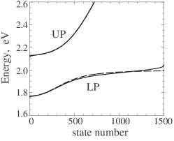
Figure 1: The energy spectrum of the polaritonic eigenstates in a 1$d$ model microcavity described by the Hamiltonian (10) with $N=1500$ molecular sites and $N=1500$ photon modes. Parameters of the systems are as follows: average exciton energy $\varepsilon=2$ eV, cavity photon cutoff energy $\Delta=1.9$ eV, dielectric constant $\epsilon=3$, the exciton-photon interaction energy $\gamma=0.15$ eV. The dashed lines show the energy eigenvalues in the system without exciton disorder, $\sigma=0$, the solid lines correspond to the spectrum in the system with disorder, $\sigma=0.03$ eV. Here the energies are shown as a function of state “number” sorted in an increasing energy order, separately for the lower (LP) and upper (UP) polariton branches. In the system without disorder, the state numbers would be immediately convertible to the corresponding wave vectors. On this scale, the UP branches of perfect and disordered systems are hardly distinguishable.

As we are actually interested in lowest energy polariton states, we will constrain further discussion mostly to the lower polariton (LP) branch. One can quickly notice that, since the photon energy (1) rapidly increases with $k$, higher-$k$ photon states would be only very weakly interacting with exciton states. Therefore a very large number of eigenstates of the system with energies close the upper end of the LP branch (see Fig. 1) are essentially reflective of the bare localized exciton states with an incoherent propagation mode. For the remaining fewer and lower energy states of the LP branch, however, the exciton-photon interaction is strong and one is then faced with an interesting interplay of the bare localized nature of the “exciton part” of the polariton and the bare coherent character of its “photon part”.

Transparent physical arguments were used in Ref. Agranovich et al., 2003 involving the indeterminacy (broadening) of the polariton wave vector $k$ owing to the exciton dephasing from the general relation:Peierls (1955)

$$\delta k=\frac{dk}{dE}\,\delta E(k)=\frac{\delta E(k)}{\hbar v_{g}(k)},$$ (2)

where $v_{g}(k)$ is the group velocity of parent polaritons in the perfect systen and $\delta E(k)$ is the energy broadening due to scattering. Based on Eq. (2), one can at least distinguish polaritonic states where $k$ is relatively well-defined in the sense of

$$\delta k\ll k.$$ (3)

If $\delta E(k)$ is weakly $k$-dependent, then, evidently from Eq. (2), condition (3) would be necessarily violated in regions of the spectrum where the group velocity $v_{g}(k)$ vanishes. For the LP branch, as seen in Fig. 1, this occurs both at its lower- and higher-energy ends. Reference Agranovich et al., 2003 provided estimates of the corresponding “end-points” $k_{\mathrm{min}}$ and $k_{\mathrm{max}}$, where $\delta k\simeq k$, for organic planar microcavities within the macroscopic electrodynamics description of polaritons. It was then anticipated that exciton scattering would render eigenstates corresponding to parent polaritons with $k<k_{\mathrm{min}}$ and $k>k_{\mathrm{max}}$ spatially localized in accordance with uncertainty relations like $\delta x\delta k_{x}\sim 1$. As we discussed above, at the higher-energy end ($k>k_{\mathrm{max}}$) of the LP branch, the eigenstates are practically bare exciton states in nature. At the lower-energy end ($k<k_{\mathrm{min}}$), one would deal with localized polaritons having comparable exciton and photon contents, particularly for the detuning $|\Delta-\varepsilon|$ small with respect to the Rabi splitting . Further numerical calculationsMichetti and Rocca (2005); Agranovich and Rocca (2005) for 1$d$ microcavities with diagonal exciton disorder confirmed this qualitative picture for the polariton states. Below, we will use a similar 1$d$ microcavity model to illustrate the nature of the low-energy LP states as well as time evolution of low-energy wave packets.

II Dynamics of low-energy wave packets in perfect microcavities

Before proceeding with a model analysis of polaritons in a disordered system, we will briefly discuss the time evolution of wave packets in perfect microcavities where all polaritons are coherent states well characterized by their wave vectors. Not only will this establish a comparative benchmark but is useful in itself as such dynamics reflects features of the polariton spectrum, and hence of the exciton-photon hybridization.

Of course, specific features of the low-energy wave packets stem from the fact that the polariton dispersion near the bottom of the LP branch ($\mathbf{k}\simeq 0$) is manifestly parabolic:

$$\omega(\mathbf{k})\simeq\omega_{0}+\alpha k^{2},\ \ \ \alpha=\hbar/2M,$$ (4)

$M$ being the cavity polariton effective mass, which makes the broadening of wave packets a relevant factor. Consider now a wave packet formed with the states close to the branch bottom:

$$U(\mathbf{r},t)=\mathrm{e}^{-i\omega_{0}t}\int d\mathbf{k}\,A(\mathbf{k})\,\mathrm{e}^{i\left(\mathbf{k}\cdot\mathbf{r}-\alpha k^{2}t\right)}.$$ (5)

It is convenient to choose the weight amplitude function $A(\mathbf{k})$ Gaussian: $A(\mathbf{k})=\left(\beta/2\pi^{3}\right)^{1/2}\exp\left[-\beta(\mathbf{k}-\mathbf{k}_{0})^{2}\right]$, centered at wave vector $\mathbf{k}_{0}$. With this amplitude function, Eq. (5) yields

$$\left|U(\mathbf{r},t)\right|^{2}=C(t)\,\exp\left[-\frac{\beta(\mathbf{r}-2\alpha\mathbf{k}_{0}t)^{2}}{2(\beta^{2}+\alpha^{2}t^{2})}\right]$$ (6)

for the time evolution of the spatial “intensity” of the wave packet,

$$C(t)=\frac{\beta}{2\pi(\beta^{2}+\alpha^{2}t^{2})}.$$

Equation (6) describes a Gaussian-shaped wave packet in 2$d$ whose center

$$\mathbf{r}_{c}(t)=\mathbf{v}_{g}t,\ \ \ \mathbf{v}_{g}=2\alpha\mathbf{k}_{0},$$

moves with the group velocity consistent with the dispersion (4), and whose linear width increases with time in accordance with the 1$d$ variance

$$s(t)=\left(\beta+\alpha^{2}t^{2}/\beta\right)^{1/2}.$$ (7)

The total energy in the wave packet is conserved: with our choice of the amplitude function,

$$\int d\mathbf{r}\left|U(\mathbf{r},t)\right|^{2}=1.$$

Of course, Eq. (6) can be derived as a product of two independent 1$d$ normalized evolutions such as

$$\left|U(x,t)\right|^{2}=\sqrt{C(t)}\,\exp\left[-\frac{\beta(x-2\alpha k_{0}t)^{2}}{2(\beta^{2}+\alpha^{2}t^{2})}\right],$$ (8)

which we will be relevant in our discussion of 1$d$ microcavities, in this case the 1$d$ packet amplitude function

$$A(k)=\left(\beta/2\pi^{3}\right)^{1/4}\exp\left[-\beta(k-k_{0})^{2}\right].$$ (9)

The spatial broadening (7) features an initial value of $\beta^{1/2}$ and a characteristic time $t_{b}=\beta/\alpha$ such that, at times $t\gg t_{b}$, the variance grows linearly with velocity $v_{b}=\alpha\beta^{-1/2}$. To appreciate the scales, some rough estimates can be made. So for the effective polariton mass $M$ on the order of $10^{-5}\,m_{0}$ ($m_{0}$ being the vacuum electron mass), parameter $\alpha=\hbar/2M\simeq 5\cdot 10^{4}$ cm²/s. Estimates in Ref. Agranovich et al., 2003 made with the Rabi splitting and detuning $\sim 100$ meV yielded for microcavities with disordered organics $k_{\mathrm{min}}\sim 10^{4}$ cm^-1. Then for the wave packets satisfying $1\lesssim\beta^{1/2}k_{\mathrm{min}}\lesssim 10$, the characteristic time would be $0.2\lesssim t_{b}\lesssim 20$ ps and the corresponding velocity $5\cdot 10^{8}\gtrsim v_{b}\gtrsim 5\cdot 10^{7}$ cm/s. In our 1$d$ numerical example below we will use the value of parameter $\beta$ within the segment just discussed.

We note that by changing physical parameters of the microcavity and organic material, as well as conditions for the polariton excitation, one can influence the dynamics described above. One should also be aware that the evolution times are limited by the actual life times $\tau$ of small wave-vector cavity polaritons. Long life times $\tau$ on the order of 10 ps can be achieved only in microcavities with high quality factors $Q=\omega\tau$.

III Time evolution in a 1$d$ microcavity with diagonal disorder

Finding polariton states in disordered planar microcavities microscopically is a difficult task which we are not attempting in this paper. As a first excursion into the study of disorder effects on polariton dynamics, here we will follow Ref. Michetti and Rocca, 2005 to explore the dynamics in a simpler microscopic model of a 1$d$ microcavity. Such microcavities are interesting in themselves and can have experimental realizations; from the results known in the theory of disordered systems,Lee and Ramakrishnan (1985) one can also anticipate that certain qualitative features may be common for 1$d$ and 2$d$ systems.

The microscopic model we study is set up in the following Hamiltonian:

$$H = \sum_{n}(\varepsilon+\varepsilon_{n})a_{n}^{{\dagger}}a_{n}+\sum_{k}\epsilon_{k}b_{k}^{{\dagger}}b_{k}$$ (10)

$$+ \gamma\sum_{nk}\sqrt{\frac{\varepsilon}{N\epsilon_{k}}}\left(\mathrm{e}^{ikna}\,a_{n}^{{\dagger}}b_{k}+\mathrm{e}^{-ikna}\,b_{k}^{{\dagger}}a_{n}\right).$$

It consists of a lattice of $N$ “molecular sites” spaced by distance $a$ and comprises the exciton part ($a_{n}$ is the exciton annihilation operator on the site $n$), photon part ($b_{k}$ is the photon annihilation operator with the wave vector $k$ and a given polarization) as well as the ordinary exciton-photon interaction. The cavity photon energy $\epsilon_{k}$ is defined by Eq. (1), $\varepsilon$ represents the average exciton energy, while $\varepsilon_{n}$ the on-site exciton energy fluctuations. We will use uncorrelated normally distributed $\varepsilon_{n}$ with the zero mean and the variance $\sigma$:

$$\langle\varepsilon_{n}\varepsilon_{m}\rangle=\sigma^{2}\delta_{nm}.$$ (11)

The exciton-photon interaction is written in such a form that $2\gamma$ yields the Rabi splitting energy in the perfect system. We chose to use the same number $N$ of photon modes, the wave vectors $k$ are discrete with $2\pi/Na$ increments. Our approach is to straightforwardly find the normalized polariton eigenstates $|\Psi_{i}\rangle$ ($i$ is the state index) of the Hamiltonian (10) and then use them in the site-coordinate representation:

$$\Psi(n)=\left(\Psi_{\mathrm{p}}(n),\,\Psi_{\mathrm{e}}(n)\right),\ \ \sum_{n}|\Psi(n)|^{2}=1,$$ (12)

where $\Psi_{\mathrm{p}}$ and $\Psi_{\mathrm{e}}$ respectively describe the photon and exciton parts of the polariton wave function and $n$ denotes the $n$th site.

We have tried various numerical parameters in the model Hamiltonian with the results being qualitatively consistent; the parameters we exploit in this paper have been chosen, on one hand, to be reasonably comparable with the experimental data in the output and, on the other hand, to better illustrate our point within a practical computational effort. It should be kept in mind though that we consider a model system and the numerical values of results may differ, likely within an order of magnitude, for various systems.

The numerical parameters are indicated in the caption to Fig. 1 and have been used to calculate the eigenstates of the Hamiltonian (10) with $N=1500$ for a cavity of the physical length $L=Na=150$ $\mu$m and a small negative detuning $(\Delta-\varepsilon)=-0.1$ eV. Figure 1 compares the energy spectra in the perfect microcavity and in the cavity with one realization of the excitonic disorder, Eq. (11), $\sigma=0.03$ eV. It is apparent that the effect of this amount of disorder on the polariton energy spectrum per se is relatively small, except in the higher-energy region of the LP branch where eigenstates, as we discussed, are practically of a pure exciton nature.

The lower-energy part of the LP branch, however, corresponds to the polariton states $\Psi$ (12) in which the exciton and photon are strongly coupled ($\gamma=0.15>|\Delta-\varepsilon|=0.1$ eV) with comparable weight contributions in $\Psi_{\mathrm{p}}$ and $\Psi_{\mathrm{e}}$. A dramatic effect of the disorder is in the strongly localized character of the polaritonic eigenstates near the bottom of the LP branch, as illustrated in Fig. 2(a) (needless to

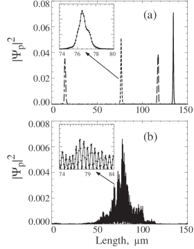
Figure 2: Examples of the spatial structure of the the photon part $|\Psi_{\mathrm{p}}|^{2}$ of the polariton eigenstates in a 1$d$ microcavity with disorder. (a) Four states, shown by different lines, from the very bottom of the LP polariton branch with energies within the range of 1.76-1.77 eV (see the spectrum in Fig. 1). The inset shows one of these states in more detail. Dots in the inset correspond to the sites of the underlying lattice. (b) One state with a higher energy close to 1.82 eV. The inset shows part of the spatial structure of this state in more detail. Dots correspond to the lattice sites and spatial oscillations of the wave function are clearly seen.

say that the same behavior is observed for the states near the bottom of the UP branch which we we are not concerned with in this paper). Of course, both the photon $\Psi_{\mathrm{p}}$ and exciton $\Psi_{\mathrm{e}}$ parts of a localized polariton state are localized on the same spatial scale, however the exciton part of the spatial wave function is more “wiggly” reflecting more the individual site energy fluctuations. For better clarity, in both Figs. 2 and 3 we show only the smoother behaving photon parts $\Psi_{\mathrm{p}}$. Panel (a) of Fig. 2 displays examples of $|\Psi_{\mathrm{p}}|^{2}$ for four states from the very bottom of the LP branch in a realization of the disordered system that are localized at different locations of the 150 $\mu$m sample. The inset to this panel shows the spatial structure of one of these states in more detail; it demonstrates both the spatial scale $l$ of localization in this energy range ($l\sim 1$ $\mu$m with the used parameters) as well as a “macroscopic” size of the localized state in comparison with the lattice spacing: $l\gg a=100$ nm.

The states at the bottom of the LP branch can be characterized as strongly localized in the sense of $kl\lesssim 1$ where $k$ is a typical wave vector of the parent polariton states in the perfect system. This feature may be contrasted to the behavior at somewhat higher energies and at higher $k>k_{\mathrm{min}}$ of parent states, where the disorder-induced indeterminacy of the $k$-vector becomes small satisfying Eq. (3) so that $k$ would appear as a good quantum number. As is known,Lee and Ramakrishnan (1985) however, the multiple scattering should still lead to spatial localization of the eigenstates, now on the spatial scale $l$ such that $kl\gg 1$. Panel (b) of Fig. 2 illustrates the spatial structure of such a state with much larger $l$ than in panel (a). The inset to panel (b) shows that the wave function in this case, within the localization length, exhibits multiple oscillations with a period on the order of $1/k$, which produces the black appearance on the scale of whole panel (b).

Having all the eigenstates of the system calculated, we are now in a position to study the time evolution of an initial polariton excitation, which we choose in the form of a wave packet $|\Psi^{0}\rangle$ built out of the low-energy polariton states $|\Psi^{0}_{i}\rangle$ of the perfect system:

$$|\Psi^{0}\rangle=\sum_{i}A_{i}\,|\Psi^{0}_{i}\rangle=\sum_{i}B_{i}\,|\Psi_{i}\rangle.$$ (13)

Polaritons in the perfect system are ordinary plane waves and we used a discretized analog of Eq. (9) for the amplitude function $A_{i}$, the result is a Gaussian-shaped wave packet as illustrated in Fig. 3 by the long-dashed lines for the photon part of the polariton wave function. Amplitudes $B_{i}$ in Eq. (13) are, on the other hand, expansion coefficients of the same initial excitation over the eigenstates $|\Psi_{i}\rangle$ of the system with disorder. The time evolution of the initial excitation in the perfect system is then given by

$$|\Psi^{0}(t)\rangle=\sum_{i}A_{i}\,\mathrm{e}^{-iE^{0}_{i}t/\hbar}\,|\Psi^{0}_{i}\rangle,$$ (14)

while the evolution in the disordered system by

$$|\Psi(t)\rangle=\sum_{i}B_{i}\,\mathrm{e}^{-iE_{i}t/\hbar}\,|\Psi_{i}\rangle,$$ (15)

where $E_{i}^{0}$ and $E_{i}$ are the respective eigenstate energies.

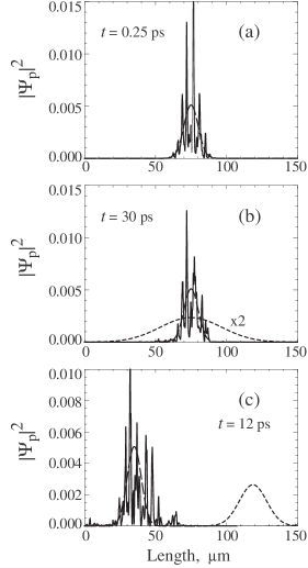
Figure 3: Examples of the the time evolution of spatially identical wave packets built out of the polariton eigenstates of a perfect 1$d$ microcavity as in Eq. (9) with the parameter $\beta^{1/2}=5$ $\mu$m. For panels (a) and (b), the initial packet has zero total momentum, $k_{0}=0$; for panel (c) the initial packet has a finite momentum determined by $k_{0}=10^{4}$ cm^-1. Only the photon part $|\Psi_{\mathrm{p}}|^{2}$ of the polariton wave function is displayed. The initial packets are shown by long-dashed lines, results of the evolution after indicated times $t$ are shown by solid lines for the disordered system and by short-dashed lines for the perfect microcavity (except in panel (a), where the latter practically coincides with the initial packet.)

Of course, the evolution of the low-energy wave packet (14) in the perfect microcavity takes place in accordance with our continuum generic description in Eq. (8) (barring small differences that may be caused by deviations from the purely parabolic spectrum). This is clearly seen in panels (b) and (c) of Fig. (3) where the photon part of $|\Psi^{0}(t)\rangle$ at indicated times $t$ is displayed by the short-dash lines: mere broadening of the wave packet with no momentum ($k_{0}=0$) in panel (b), and both broadening and translational displacement ($k_{0}\neq 0$) in panel (c). On the time scale of panel (a), the $|\Psi^{0}(t)\rangle$ state has not practically evolved yet from $|\Psi^{0}\rangle$ and is not shown on that panel.

The time evolution of exactly the same initial polariton packets is drastically different in the disordered system, the corresponding spatial patterns of the photon part of $|\Psi(t)\rangle$ are shown in Fig. 3 with solid lines. First of all, the initial packet is quickly (faster than a fraction of ps) transformed into a lumpy structure reflecting the multitude of the localized polariton states within the spatial region of the initial excitation. Note that in our illustration here we intentionally chose the initial amplitude function (9) with the parameter $\beta^{1/2}=5$ $\mu$m large enough for the spatial size of the initial excitation to be much larger than the size of the individual localized polaritons at these energies (compare to Fig. 2(a)). Importantly, however, that, while displaying some internal dynamics (likely resulting from the overlap of various localized states), this lumpy structure does not propagate well beyond the initial excitation region over longer times. This is especially evident in comparison, when the broadening and motion of the packets in the perfect system is apparent (panels (b) and (c) of Fig. 3). We have run simulations over extended periods of time ($\sim 100$ ps) with the result that $|\Psi(t)\rangle$ remains essentially localized within the same spatial region. Of course, some details of $|\Psi(t)\rangle$ depend on the initial excitation - see, e.g., a somewhat broader localization region in Fig. 3(c) for the initial excitation with an initial momentum corresponding to $k_{0}=10^{4}$ cm^-1 but the long-term localization in the disordered system appears robust in all our simulations. It would be interesting to extend the dynamical studies with participation of higher energy states such as in Fig. 2(b), this is, however, beyond the scope of the present paper.

IV Concluding remarks

The nature and dynamics of low-energy cavity polariton states are important for various physical processes in microcavities, particularly for the problem of condensation of polaritons into the lowest energy state(s). As was demonstrated in Ref. Agranovich et al., 2003, low-energy polaritons in organic microcavities should be especially susceptible to effects of scattering/disorder in the exciton subsystem. The problem of disorder effects on polaritons in organic microcavities appears quite interesting as organic materials would typically feature both strong exciton-photon coupling and substantial static and/or dynamic exciton scattering. In this paper we have continued a line of study in Ref. Michetti and Rocca, 2005 to look in some more detail at disorder effects on polaritons in a 1$d$ model microcavity. Our numerical analysis has brought further evidence that low-energy polariton states in organic microcavities can be strongly localized in the sense of $l\lesssim\lambda$, where $l$ is the spatial size of localized states and $\lambda$ the wave length of parent polariton waves. (We have also found indications of weaker localization at higher polariton energies in the sense of $l\gg\lambda$.) Our illustrations have included demonstrations of localization not only via the spatial appearance of polariton eigenstates but also via the time evolution of different low-energy wave packets.

On the physical grounds,Agranovich et al. (2003) one should expect that low-energy polaritons in 2$d$ organic microcavities would also be rendered strongly localized by disorder, as it would also follow from the general ideas of the theory of localization.Lee and Ramakrishnan (1985) Further work on microscopic models of 2$d$ polariton systems is required to quantify their localization regimes.

The strongly localized nature of low-energy polariton states should affect many processes such as light scattering and nonlinear phenomena as well as temperature-induced diffusion of polaritons. Manifestations of the localized polariton statistics (Frenkel excitons are paulions exhibiting properties intermediate between fermi and bose particles) in the problem of condensation also appear interesting and important.

We note that one can exercise an experimental control over the degree of exciton-photon hybridization and disorder by modifying the size of microcavity for various organic materials making such systems a fertile ground for detailed experimental and theoretical research into their physics.

And the last remark. While we have specifically discussed exciton-photon polaritons in organic systems, it is clear that some aspects have a generic character and could be applicable to other systems. This, for instance, concerns inorganic semiconductor microcavities. Both exciton-photon coupling and magnitudes of disorder there, however, are much smaller, which would likely make any localization effects relevant only at very low temperatures. As one of recent examples of a very different kind of systems, we will mention hybrid modes in chains of noncontacting noble metal nanoparticles where the interaction of photons and nanoparticles lead to plasmon-polaritons.Citrin and Back (2006)

V Acknowledgements

VMA’s work was supported by Russian Foundation of Basic Research and Ministry of Science and Technology of Russian Federation. He is also grateful to G. C. La Rocca for discussions. The authors thank D. Basko for reading and commenting on the manuscript.

References

- Burstein and Weisbuch (1995) E. Burstein and C. Weisbuch, eds., Confined Electrons and Photons: New Physics and Applications (Plenum, New York, 1995).
- Weisbuch and Rarity (1996) C. Weisbuch and J. G. Rarity, eds., Microcavities and Photonic Bandgaps: Physics and Applications (Kluwer, Dordrecht, 1996).
- Skolnick et al. (1998) M. S. Skolnick, T. A. Fisher, and D. M. Whittaker, Semicond. Sci. Technol. 13, 645 (1998).
- Khitrova et al. (1999) G. Khitrova, H. M. Gibbs, F. Jahnke, M. Kira, and S. W. Koch, Rev. Mod. Phys. 71, 1591 (1999).
- Kavokin and Malpuech (2003) A. Kavokin and G. Malpuech, Cavity Polaritons (Elsevier, Amsterdam, 2003).
- Bassani (2003) F. Bassani, in Electronic excitations in organic based nanostructures, edited by V. M. Agranovich and F. Bassani (Elsevier, Amsterdam, 2003), p. 129.
- Weisbuch and Benisty (2005) C. Weisbuch and H. Benisty, Solid State Commun. 135, 627 (2005).
- Tassone et al. (1997) F. Tassone, C. Piermarocchi, V. Savona, A. Quattropani, and P. Schwendimann, Phys. Rev. B 56, 7554 (1997).
- Imamoglu et al. (1996) A. Imamoglu, R. J. Ram, S. Pau, and Y. Yamamoto, Phys. Rev. A 53, 4250 (1996).
- Yamamoto (2000) Y. Yamamoto, Nature 405, 629 (2000).
- Savvidis et al. (2000a) P. G. Savvidis, J. J. Baumberg, R. M. Stevenson, M. S. Skolnick, D. M. Whittaker, and J. S. Roberts, Phys. Rev. Lett. 84, 1547 (2000a).
- Stevenson et al. (2000) R. M. Stevenson, V. N. Astratov, M. S. Skolnick, D. M. Whittaker, M. Emam-Ismail, A. I. Tartakovskii, P. G. Savvidis, J. J. Baumberg, and J. S. Roberts, Phys. Rev. Lett. 85, 3680 (2000).
- Savvidis et al. (2000b) P. G. Savvidis, J. J. Baumberg, R. M. Stevenson, M. S. Skolnick, D. M. Whittaker, and J. S. Roberts, Phys. Rev. B 62, R13278 (2000b).
- Alexandrou et al. (2001) A. Alexandrou, G. Bianchi, E. Péronne, B.Hallé, F. Boeuf, R. André, R. Romestein, and L. S. Dang, Phys. Rev. B 64, 233318 (2001).
- Deng et al. (2002) H. Deng, G. Weihs, and C. Santori, Science 298, 199 (2002).
- Rubo et al. (2003) Y. Rubo, F. P. Laussy, A. Kavokin, and P. Bigenwald, Phys. Rev. Lett. 91, 156403 (2003).
- Laussy et al. (2004) F. P. Laussy, G. Malpuech, A. Kavokin, and P. Bigenwald, Phys. Rev. Lett. 93, 016402 (2004).
- Lidzey et al. (1998) D. G. Lidzey, D. D. C. Bradley, M. S. Skolnick, T. Virgili, S. Walker, and D. M. Whittaker, Nature 395, 53 (1998).
- Lidzey et al. (1999) D. G. Lidzey, D. D. C. Bradley, M. S. Skolnick, T. Virgili, S. Walker, and D. M. Whittaker, Phys. Rev. Lett. 82, 3316 (1999).
- Tartakovskii et al. (2001) A. I. Tartakovskii, M. Emam-Ismail, D. G. Lidzey, M. S. Skolnik, D. D. C. Bradley, S. Walker, and V. M. Agranovich, Phys. Rev. B 63, 121302 (2001).
- Hobson et al. (2002) P. A. Hobson, W. L. Barnes, D. G. Lidzey, G. A. Gehring, D. M. Whittaker, M. S. Skolnick, and S. Walker, Appl. Phys. Lett. 81, 3519 (2002).
- Schouwink et al. (2002) P. Schouwink, J. Lupton, H. von Berlepsch, L. Dahne, and R. F. Mahr, Phys. Rev. B 66, 081203(R) (2002).
- Lidzey et al. (2002) D. G. Lidzey, A. M. Fox, M. D. Rahn, M. S. Skolnik, V. M. Agranovich, and S. Walker, Phys. Rev. B 65, 195312 (2002).
- Takada et al. (2003) N. Takada, T. Kamata, and D. D. C. Bradley, Appl. Phys. Lett. 82, 1812 (2003).
- Lidzey (2002) D. G. Lidzey, in Organic Nanostructures: Science and Applications, edited by V. M. Agranovich and G. C. L. Rocca (IOS Press, Amsterdam, 2002), p. 405.
- Lidzey (2003) D. G. Lidzey, in Electronic excitations in organic based nanostructures, edited by V. M. Agranovich and F. Bassani (Elsevier, Amsterdam, 2003), ch. 8.
- Holmes and Forrest (2004) R. J. Holmes and S. R. Forrest, Phys. Rev. Lett. 93, 186404 (2004).
- Holmes and Forrest (2005) R. J. Holmes and S. R. Forrest, Phys. Rev. B 71, 235203 (2005).
- Agranovich et al. (2003) V. M. Agranovich, M. Litinskaia, and D. G. Lidzey, Phys. Rev. B 67, 085311 (2003).
- Peierls (1955) R. E. Peierls, Quantum Theory of Solids (Clarendon, Oxford, 1955).
- Michetti and Rocca (2005) P. Michetti and G. C. L. Rocca, Phys. Rev. B 71, 115320 (2005).
- Agranovich and Rocca (2005) V. M. Agranovich and G. C. L. Rocca, Solid State Commun. 135, 544 (2005).
- Lee and Ramakrishnan (1985) P. A. Lee and T. V. Ramakrishnan, Rev. Mod. Phys. 57, 287 (1985).
- Citrin and Back (2006) D. S. Citrin and T. D. Back, phys. stat. sol. (b) 243, 2349 (2006).