Alleviation of the Fermion-sign problem by optimization of many-body wave functions

Abstract

We present a simple, robust and highly efficient method for optimizing all parameters of many-body wave functions in quantum Monte Carlo calculations, applicable to continuum systems and lattice models. Based on a strong zero-variance principle, diagonalization of the Hamiltonian matrix in the space spanned by the wave function and its derivatives determines the optimal parameters. It systematically reduces the fixed-node error, as demonstrated by the calculation of the binding energy of the small but challenging C₂ molecule to the experimental accuracy of 0.02 eV.

Many important problems in computational physics and chemistry can be reduced to the computation of the dominant eigenvalues of matrices or integral kernels. For problems with many degrees of freedom, Monte Carlo approaches such as diffusion, reptation and transfer-matrix Monte Carlo are among the most accurate and efficient methods Pro . Their efficiency and in most cases accuracy rely crucially on good approximate eigenstates. For Fermionic systems, the antisymmetry constraint leads to the Fermion-sign problem that forces practical implementations to fix the nodes to those of an approximate trial wave function. The resulting fixed-node error is the main uncontrolled error in quantum Monte Carlo (QMC). Despite great effort aimed at developing algorithms that eliminate this error entirely D. M. Ceperley and B. J. Alder, J. Chem. Phys. 81, 5833 ; Shiwei Zhang and M. H. Kalos, Phys. Rev. Lett. 71, 2159 (1993);() (1984), to date there is no generally applicable solution, therefore systematic improvement of the wave function by optimization of an increasing number of variational parameters is the most practical approach for reducing this error.

In this letter we develop a robust and highly efficient method for optimizing all parameters in approximate wave functions. Application to the small but challenging C₂ molecule demonstrates that the method systematically eliminates the fixed-node error. The method is based on energy minimization in variational Monte Carlo (VMC) and extends the zero-variance linear optimization method M. P. Nightingale and V. Melik-Alaverdian (2001) to nonlinear parameters. The approach is simpler than the Newton method C. J. Umrigar and C. Filippi (2005) as it does not require second derivatives of the wave function. Moreover, in contrast to the perturbative optimization method Scemama and Filippi (2006), it enables the simultaneous parameter optimization of both the Jastrow and the determinantal parts of the wave function with equal efficiency.

Form of wave functions.   We employ $N$-electron wave functions which depend on $N_{\rm opt}$ variational parameters collectively denoted by ${\bf p}=({\bf c},\bm{\alpha},\bm{\lambda})$ and $3N$ electronic coordinates, ${\bf R}$,

$$\Psi({\bf p},{\bf R})=J(\bm{\alpha},{\bf R})\sum_{i=1}^{N_{\rm CSF}}c_{i}C_{i}(\bm{\lambda},{\bf R}),$$ (1)

where $J(\bm{\alpha},{\bf R})$ is a Jastrow factor that contains electron-nuclear, electron-electron and electron-electron-nuclear terms. Each of the $N_{\rm CSF}$ configuration state functions (CSFs), $C_{i}(\bm{\lambda},{\bf R})$, is a symmetry-adapted linear combination of Slater determinants of single-particle orbitals $\phi_{\mu}({\bf r})$ which are themselves expanded in terms of $N_{\rm basis}$ basis functions $\chi_{\nu}({\bf r})$: $\phi_{\mu}({\bf r})=\sum_{\nu=1}^{N_{\rm basis}}\lambda_{\mu\nu}\chi_{\nu}({\bf r})$. The variational parameters are the linear CSF coefficients ${\bf c}$, and the nonlinear Jastrow parameters $\bm{\alpha}$ and expansion coefficients of the orbitals $\bm{\lambda}$. In practice, we optimize only $N_{\rm CSF}-1$ CSF coefficients (as the normalization of the wave function is irrelevant) and a set of non-redundant orbital rotation parameters Schautz and Filippi (2004); J. Toulouse and C. J. Umrigar .

Optimization of wave functions.   We extend the zero-variance method of Nightingale and Alaverdian M. P. Nightingale and V. Melik-Alaverdian (2001) for linear parameters to nonlinear parameters. At each optimization step, the wave function is expanded to linear-order in $\Delta{\bf p}={\bf p}\!-\!{\bf p}^{0}$ around the current parameters ${\bf p}^{0}$,

$$\Psi_{\text{lin}}({\bf p},{\bf R})=\Psi_{0}({\bf R})+\sum_{i=1}^{N_{\rm opt}}\Delta p_{i}\,\Psi_{i}({\bf R}),$$ (2)

where $\Psi_{0}=\Psi({\bf p}_{0})$ is the current wave function and $\Psi_{i}=\left(\partial\Psi({\bf p})/\partial p_{i}\right)_{{\bf p}={\bf p}_{0}}$ are the $N_{\rm opt}$ derivatives of the wave function with respect to the parameters. On an infinite Monte Carlo (MC) sample, the parameter variations $\Delta{\bf p}$ minimizing the energy calculated with the linearized wave function of Eq. (2) are the lowest eigenvalue solution of the generalized eigenvalue equation

$${\bf H}\Delta{\bf p}=E\,{\bf S}\Delta{\bf p},$$ (3)

where ${\bf H}$ and ${\bf S}$ are the Hamiltonian and overlap matrices in the ($N_{\rm opt}+1$)-dimensional basis formed by the current wave function and its derivatives $\left\{\Psi_{0},\Psi_{1},\Psi_{2},\cdots,\Psi_{N_{\rm opt}}\right\}$ and $\Delta p_{0}=1$. On a finite MC sample, following Ref. M. P. Nightingale and V. Melik-Alaverdian, 2001, we estimate these matrices by

$$H_{ij}=\left\langle{\Psi_{i}\over\Psi_{0}}{H\Psi_{j}\over\Psi_{0}}\right\rangle_{\Psi_{0}^{2}},\;\;\;\;\;S_{ij}=\left\langle{\Psi_{i}\over\Psi_{0}}{\Psi_{j}\over\Psi_{0}}\right\rangle_{\Psi_{0}^{2}},$$ (4)

where $H$ is the electronic Hamiltonian. We employ the notation that $\left\langle{\Psi_{i}\over\Psi_{0}}{A\Psi_{j}\over\Psi_{0}}\right\rangle_{\Psi_{0}^{2}}$ denotes the statistical estimate of $\langle\Psi_{i}|\hat{A}|\Psi_{j}\rangle/\langle\Psi_{0}|\Psi_{0}\rangle$ evaluated using MC configurations sampled from $\Psi_{0}^{2}$. The estimator for the matrix ${\bf H}$ in Eq. (4) is nonsymmetric and is not the symmetric Hamiltonian matrix that one would obtain by minimizing the energy of the finite MC sample. In fact, as shown in Ref. M. P. Nightingale and V. Melik-Alaverdian, 2001, it is only this nonsymmetric estimator for ${\bf H}$ that leads to a strong zero-variance principle: the variance of the parameter changes $\Delta{\bf p}$ in Eq. (3) vanishes not only in the limit that $\Psi_{0}$ is the exact eigenstate but even in the limit that $\Psi_{\rm lin}$ with optimized parameters is an exact eigenstate. In practice, for the wave functions we employ, and optimizing on small MC samples, the asymmetric Hamiltonian results in 1 to 2 orders of magnitude smaller fluctuations in the parameter values.

Quite generally, methods that minimize the energy of a finite MC sample are stable only if a much larger number of MC configurations is employed than is necessary for the variance minimization method C. J. Umrigar, K. G. Wilson and J. W. Wilkins (1988) because the energy of a finite sample is not bounded from below but the variance is. However, it is possible to devise simple modifications of these energy-minimization methods that require orders of magnitude fewer MC configurations. Both the zero-variance linear method employed here and the modified Newton method C. J. Umrigar and C. Filippi (2005) are examples of such modifications.

Having obtained the parameter variations $\Delta{\bf p}$ by solving Eq. (3), there is no unique way to update the parameters in the wave function. The simplest procedure of incrementing the current parameters by $\Delta{\bf p}$, ${\bf p}_{0}\to{\bf p}_{0}+\Delta{\bf p}$ works for the linear parameters but is not guaranteed to work for the nonlinear parameters if the linear approximation of Eq. (2) is not good. A better but more complicated procedure is to fit the original wave function form to the optimal linear combination. We next discuss a simple prescription that avoids doing this fit.

At first, it may appear that nothing can be done to make the linear approximation better, but this is in fact not the case. One can exploit the freedom of the normalization of the wave function to alter the dependence on the nonlinear parameters as follows. Consider the differently-normalized wave function $\overline{\Psi}({\bf p},{\bf R})=N({\bf p})\Psi({\bf p},{\bf R})$ such that $\overline{\Psi}({\bf p}_{0},{\bf R})=\Psi({\bf p}_{0},{\bf R})\equiv\Psi_{0}({\bf R})$ and $N({\bf p})$ depends only on the nonlinear parameters. Then, the derivatives of $\overline{\Psi}({\bf p})$ are

$$\overline{\Psi}_{i}=\Psi_{i}+N_{i}\Psi_{0},\hbox{\hskip 8.53581ptwhere \hskip 8.53581pt}N_{i}=\left(\partial N({\bf p})/\partial p_{i}\right)_{{\bf p}={\bf p}_{0}},$$ (5)

with $N_{i}=0$ for linear parameters. The first-order expansion of $\overline{\Psi}({\bf p})$ after optimization is

$$\overline{\Psi}_{\text{lin}}=\Psi_{0}+\sum_{i=1}^{N_{\rm opt}}\Delta{\bar{p}}_{i}\,\overline{\Psi}_{i}.$$ (6)

Since $\overline{\Psi}_{\text{lin}}$ and $\Psi_{\text{lin}}$ were obtained by optimization in the same variational space they must be proportional to each other, so $\Delta{\bar{\bf p}}$ are related to $\Delta{\bf p}$ by a uniform rescaling

$$\Delta{\bar{\bf p}} = {\Delta{\bf p}\over 1-\sum_{i=1}^{N_{\rm opt}}N_{i}\Delta p_{i}}.$$ (7)

Since the rescaling factor can be anywhere between $-\infty$ and $\infty$ the choice of normalization can affect not only the magnitude of the parameter changes but even the sign.

For the nonlinear parameters, we have found that, in all cases considered here, a fast and stable optimization is achieved if $N_{i}$ are determined by imposing the condition that each derivative $\overline{\Psi}_{i}$ is orthogonal to a linear combination of $\Psi_{0}$ and $\Psi_{\text{lin}}$, i.e., $\langle\xi{\Psi_{0}\over||\Psi_{0}||}+(1-\xi){\Psi_{\text{lin}}\over||\Psi_{\text{lin}}||}|\overline{\Psi}_{i}\rangle=0$, where $\xi$ is a constant between 0 and 1, resulting in

$$N_{i} = -{\xi DS_{0i}+(1-\xi)(S_{0i}+\sum_{j}^{\rm nonlin}S_{ij}\Delta p_{j})\over\xi D+(1-\xi)(1+\sum_{j}^{\rm nonlin}S_{0j}\Delta p_{j})},$$ (8)

with $D=\sqrt{1+2\sum_{j}^{\rm nonlin}S_{0j}\Delta p_{j}+\sum_{j,k}^{\rm nonlin}S_{jk}\Delta p_{j}\Delta p_{k}}$, where the sums are over only the nonlinear parameters. The simple choice $\xi=1$ first used by Sorella in the context of the stochastic reconfiguration method Sorella (2001) leads in many cases to good parameter variations, but in some cases can result in arbitrarily large parameter variations that may or may not be desirable. The safer choice $\xi=0$ minimizes the norm of the linear wave function change $||\overline{\Psi}_{\text{lin}}-\Psi_{0}||$ in the case that only the nonlinear parameters are varied, but, it can yield arbitrarily small parameter changes even far from the energy minimum. In contrast, the choice $\xi=1/2$, imposing $||\overline{\Psi}_{\text{lin}}||=||\Psi_{0}||$, guarantees finite parameter changes, until the energy minimum is reached.

If instead of finding the parameter changes from Eqs. (3) and (7) one expands the Rayleigh quotient $\langle\bar{\Psi}_{\rm lin}|\hat{H}|\bar{\Psi}_{\rm lin}\rangle/\langle\bar{\Psi}_{\rm lin}|\bar{\Psi}_{\rm lin}\rangle$ with $\xi=1$ to second order in $\Delta{\bar{\bf p}}$ one recovers the stochastic reconfiguration with Hessian acceleration (SRH) method with $\beta=0$ of Ref. Sorella, 2005. It turns out that the SRH method is much less stable and converges more slowly, particularly for large systems with many parameters.

Stabilization of the optimization.   When the parameter values are far from optimal or if the MC sample used to evaluate the ${\bf H}$ and ${\bf S}$ matrices is very small, then the updated parameters may be worse than the original ones. However, it is possible to devise a scheme to stabilize the method in a manner similar to that used for the modified Newton method C. J. Umrigar and C. Filippi (2005). Stabilization is achieved by adding a positive constant, $a_{\rm diag}\geq 0$, to the diagonal of the Hamiltonian matrix except for the first element: $H_{ij}\to H_{ij}+a_{\rm diag}\delta_{ij}(1-\delta_{i0})$. As $a_{\rm diag}$ becomes larger the parameter variations $\Delta{\bf p}$ become smaller and rotate towards the steepest descent direction. In practice, the value of $a_{\rm diag}$ is automatically adjusted at each optimization step. Once the matrices ${\bf H}$ and ${\bf S}$ have been computed, three values of $a_{\rm diag}$ differing from each other by factors of 10 are used to predict three new wave functions. A short MC run is then performed using correlated sampling to compute energy differences of these wave functions more accurately than the energy itself. The optimal value of $a_{\rm diag}$ is then calculated by parabolic interpolation on these three energies, with some bounds imposed.

Results.   We demonstrate the performance of our optimization method on the ${}^{1}\Sigma_{g}^{+}$ ground state of the C₂ molecule at the experimental equilibrium interatomic distance of $2.3481$ Bohr, employing a scalar-relativistic Hartree-Fock (HF) pseudopotential Burkatzki et al. with a large Gaussian polarized valence quintuple-zeta one-electron basis (12 $s$, 10 $p$ and 4 $d$ functions contracted to 5 $s$, 5 $p$ and 4 $d$ functions) to ensure basis-set convergence. The quantum chemistry package GAMESS M. W. Schmidt et al. (1993) is used to obtain multi-configurational self-consistent field (MCSCF) wave functions in complete active spaces (CAS) generated by distributing $n$ valence electrons in $m$ orbitals [CAS($n$,$m$)]. We also employ restricted active space RAS($n$,$m$) wave functions consisting of a truncation of the CAS($n$,$m$) wave functions to quadruple excitations. By applying a variable cutoff on the CSF coefficients, only the Slater determinants with the largest CSF coefficients are retained in these wave functions, which are then multiplied by a Jastrow factor with essentially all free parameters chosen to be zero to form our starting trial wave functions.

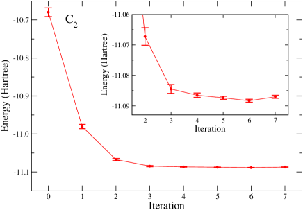
Figure 1: Convergence of the VMC total energy of the C₂ molecule with a HF pseudopotential Burkatzki et al. when simultaneously optimizing 24 Jastrow, 73 CSF and 174 orbital parameters for a truncated CAS(8,14) wave function. The insert is an enlargement of the last iterations.

Fig. 1 illustrates the convergence of the VMC energy during the simultaneous optimization of 24 Jastrow, 73 CSF and 174 orbital parameters for a truncated CAS(8,14) wave function. The energy converges to an accuracy of about $10^{-3}$ Hartree in 5 iterations, making it the most rapidly convergent method for optimizing all the parameters in Jastrow-Slater wave functions.

Figure 2: (Color online) VMC and DMC total energies of the C₂ and Si₂ molecules, versus the number of determinants in truncated Jastrow-Slater CAS(8,14) wave functions, for different levels of optimization. Both VMC and DMC energies decrease monotonically if the CSF coefficients are reoptimized in VMC but not if only the Jastrow factor is optimized.

Fig. 2 shows the total VMC and DMC energies of the C₂ molecule as a function of the number of determinants retained in truncated Jastrow-Slater CAS(8,14) wave functions. For comparison, the convergence of the ${}^{3}\Sigma_{g}^{+}$ ground state energy of Si₂ is also shown. For each of VMC and DMC, there are three curves. For the upper curve, only the Jastrow parameters are optimized and the CSF and orbital coefficients are fixed at their MCSCF values. For the middle curve, the Jastrow and CSF parameters are optimized simultaneously while, for the lower curve, the Jastrow, CSF and orbital parameters are optimized simultaneously. With fixed CSF coefficients, the energy does not improve monotonically with the number of determinants. In contrast, if the CSF coefficients are reoptimized then of course the VMC energy improves monotonically. Remarkably, so does the DMC energy, implying that the nodal hypersurface of the wave function is monotonically improved even though only the VMC energy is explicitly optimized.

The difference in the behaviors of the C₂ and Si₂ molecules is striking. While for Si₂ the energy shows a small gradual decrease upon increasing the number of determinants, for C₂ there is a very rapid initial decrease, a manifestation of the presence of strong energetic near-degeneracies among valence orbitals. The fixed-node error of a single-determinant wave function using MCSCF natural orbitals is about $6$ mHa for Si₂ and about $46$ mHa for C₂, almost an order of magnitude larger!

Retaining all the determinants of a CAS(8,14) wave function would be costly in QMC but one can estimate the energy in this limit by extrapolation. Fig. 3 shows a quadratic fit of the VMC and DMC energies obtained with truncated, fully reoptimized wave functions with respect to the sum of the squares of the MCSCF CSF coefficients retained, $\sum_{i=1}^{N_{\rm CSF}}(c_{i}^{\text{MCSCF}})^{2}$. This sum is equal to $1$ in the limit that all the CSFs are included.

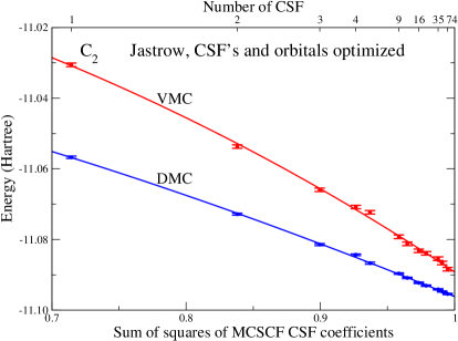
Figure 3: (Color online) Extrapolation (to $1$) by quadratic fits of the VMC and DMC energies obtained with the truncated, fully reoptimized Jastrow-Slater CAS(8,14) wave functions with respect to the sum of the squares of the MCSCF CSF coefficients retained, $\sum_{i=1}^{N_{\rm CSF}}(c_{i}^{\text{MCSCF}})^{2}$.

Table 1: Total energy and well depth of the C₂ molecule, with a HF pseudopotential Burkatzki et al. , obtained in DMC with a series of fully optimized Jastrow-Slater wave functions. The well depth in column 3 is obtained using a well-converged DMC atomic energy, -5.43401(6) H, whereas that in column 4 uses atomic CAS wave functions consistent with the molecular ones in order to achieve some cancellation of error.

Wave function	Total energy (H)	Well depth (eV)
1 determinant	-11.0566(3)	5.13(1)	5.70(1)
CAS(8,8)	-11.0922(3)	6.10(1)	6.39(1)
CAS(8,10)	-11.0939(3)	6.15(1)	6.37(1)
CAS(8,14)	-11.0962(3)	6.21(1)	6.38(1)
CAS(8,18)	-11.0986(3)	6.28(1)	6.36(1)
RAS(8,26)	-11.1007(3)	6.33(1)	–
Estimated exacta	–	6.36(2)	6.36(2)
a Scalar-relativistic, valence-corrected estimate of Ref. Bytautas and Ruedenberg, 2005.

Table 1 reports the extrapolated DMC energies and well depths (dissociation energy + zero-point energy) for a series of fully optimized Jastrow-Slater CAS and RAS wave functions. Increasing the size of the active space results in a monotonic improvement of the total energy and the well depth in column 3 obtained using a good estimate of the exact atomic energy from a DMC calculation with a CAS(4,13) wave function. Chemical accuracy (1 kcal/mol = 0.04 eV) is reached for the largest active space. Alternatively, as shown in column 4, good well depths can be obtained using much smaller active spaces by relying on a partial cancellation of error employing atomic wave functions consistent with the molecular ones: for the molecular single determinant wave function, an atomic single determinant wave function is also used; for the molecular CAS(8,$m$) wave functions, atomic CAS(4,$m$/2) wave functions are used. In this case, while the use of a single-determinant wave function yields an error of 0.66 eV, all the CAS wave functions yield well-depths that agree with the exact one to better than chemical accuracy. This behavior parallels the standard quantum chemistry approaches where single-determinant reference methods such as coupled cluster are in error by as much as 0.2 eV while multi-reference configuration interaction calculations yield chemical accuracy Bytautas and Ruedenberg (2005). Density functional theory methods on the other hand perform rather poorly, giving a well depth of 6.69 and 4.69 eV within LDA and B3LYP, respectively.

Conclusions.   The method presented provides a systematic means of eliminating the main limitation of present-day QMC calculations, namely the fixed-node error, and supercedes variance minimization C. J. Umrigar, K. G. Wilson and J. W. Wilkins (1988) as the method of choice for optimizing many body wave functions. Extension of the method to geometry optimization will overcome the other major limitation of QMC methods.

Acknowledgments.   We thank M. P. Nightingale, R. Assaraf and A. Savin for discussions. Computations were performed at NERSC, NCSA, OSC and CNF. Supported by NSF (DMR-0205328, EAR-0530301), Sandia Natl. Lab., FOM (Netherlands) and MIUR-COFIN05.

References

- (1) W. M. C. Foulkes, L. Mitas, R. J. Needs and G. Rajagopal, Rev. Mod. Phys., 73, 33 (2001); M. P. Nightingale and C. J. Umrigar, eds., Quantum Monte Carlo Methods in Physics and Chemistry, NATO ASI Ser. C 525 (Kluwer, Dordrecht, 1999); S. Baroni and S. Moroni, Phys. Rev. Lett. 82, 4745 (1999); M.P. Nightingale and H. Blöte, Phys. Rev. Lett. 60, 1662 (1988).
- D. M. Ceperley and B. J. Alder, J. Chem. Phys. 81, 5833 ; Shiwei Zhang and M. H. Kalos, Phys. Rev. Lett. 71, 2159 (1993);() (1984) D. M. Ceperley and B. J. Alder, J. Chem. Phys. 81, 5833 (1984); Shiwei Zhang and M. H. Kalos, Phys. Rev. Lett. 71, 2159 (1993);, J. B. Anderson in Quantum Monte Carlo: Atoms, Molecules, Clusters, Liquids and Solids, Reviews in Computational Chemistry, Vol. 13, ed. by K. B. Lipkowitz and D. B. Boyd (1999).
- M. P. Nightingale and V. Melik-Alaverdian (2001) M. P. Nightingale and V. Melik-Alaverdian, Phys. Rev. Lett. 87, 043041 (2001).
- C. J. Umrigar and C. Filippi (2005) C. J. Umrigar and C. Filippi, Phys. Rev. Lett. 94, 150201 (2005).
- Scemama and Filippi (2006) A. Scemama and C. Filippi, Phys. Rev. B 73, 241101 (2006).
- (6) J. Toulouse and C. J. Umrigar, unpublished.
- Schautz and Filippi (2004) F. Schautz and C. Filippi, J. Chem. Phys. 120, 10931 (2004).
- C. J. Umrigar, K. G. Wilson and J. W. Wilkins (1988) C. J. Umrigar, K. G. Wilson and J. W. Wilkins, Phys. Rev. Lett. 60, 1719 (1988).
- Sorella (2001) S. Sorella, Phys. Rev. B 64, 024512 (2001).
- Sorella (2005) S. Sorella, Phys. Rev. B 71, 241103 (2005).
- (11) M. Burkatzki, C. Filippi, and M. Dolg, unpublished.
- M. W. Schmidt et al. (1993) M. W. Schmidt et al., J. Comp. Phys. 14, 1347 (1993).
- Bytautas and Ruedenberg (2005) L. Bytautas and K. Ruedenberg, J. Chem. Phys. 122, 154110 (2005).