Exciton luminescence in resonant photonic crystals

Abstract

A phenomenological theory of luminescence properties of one-dimensional resonant photonic crystals is developed within the framework of classical Maxwell equations with fluctuating polarization terms representing non-coherent sources of emission. The theory is based on an effective general approach to determining linear response of these structures and takes into account formation of polariton modes due to coherent radiative coupling between their constituting elements. The general results are applied to Bragg multiple-quantum-well structures, and theoretical luminescence spectra of these systems are compared with experimental results. It is shown that the emission of such systems can be significantly influenced by deliberately introducing defect elements in the structure. The relation between absorption and luminescence spectra is also discussed.

I Introduction

A possibility to influence the emission of light by tailoring the dielectric environment of emitting objects has been attracting a great deal of attention since a pioneering work by Yablonovitch. Yablonovitch (1987) In Ref. Yablonovitch, 1987 it was suggested that a three-dimensional periodic modulation of the dielectric constant can result in formation of a photonic band structure, consisting of allowed and forbidden photonic bands in analogy with electronic band structure. One of the important consequences of the band structure is a modification of electromagnetic density of states, which can be used to suppress or enhance the rate of the spontaneous emission of emitters embedded in a photonic crystal. While such drastic effects as the full inhibition of the spontaneous emission proved to be difficult to achieve,Joannopoulos et al. ; Woldeyohannes and John (2003) there is still a growing interest in emission properties of photonic crystals,Megens et al. (1999); Li and Zhang (2001); Florescu and John (2001); Vats et al. (2002); Barth et al. (2006) which even in the absence of complete photonic band-gap may result in a significant modification of properties of emitted radiation. If one is not looking to achieve the full inhibition of the spontaneous emission, the systems in which a periodic modulation takes place in only two or even one dimension are also of interest, because even though they cannot confine light completely, they do modify emission patterns for particular directions, which can be useful for various applications.

One-dimensional structures attract a particularly great attention, firstly, because they are easiest to manufacture, and secondly, because they allow for a detailed theoretical description. These two circumstances make one-dimensional structures most suitable candidates for a number of applications that do not require modification of the electromagnetic properties in all three dimensions. At the same time, certain properties of one-dimensional structures are typical for two- and three-dimensional systems as well, and, therefore, these structures provide a convenient testing area for understanding some general properties of media with spatial modulation of the dielectric function.

Most of the previous works addressed the problem of the spontaneous emission in 1D photonic structures from the perspective of individual emitters embedded in special dielectric environments such as superlattices or a Fabry-Perot cavities (see, for instance, Refs. Brueck et al., 2003; Hoekstra and Elrofai, 2005; Savona et al., 1996; Hayes et al., 1998 and references therein). Theoretical analysis of these situations is based on the assumption that the structure of photonic modes is determined solely by the periodical modulation of the dielectric function. The interaction between the photonic modes and emitters is considered in this approach as weak in a sense, that it does not affect the structure of the photonic modes, and can be treated perturbatively within the framework of Fermi Golden Rule.

These assumptions, however, break down in the important case of so called resonant photonic crystals, that have begun attracting considerable attention in recent years. These structures are composed of periodically distributed structural elements containing dipole active internal excitations, which co-exist with periodic modulation of the dielectric constant.Kuzmiak and Maradudin (1997); Deych et al. (1998); Nojima (2000); Sivachenko et al. (2001); Christ et al. (2003); Huang et al. (2003); Toader and John (2004); Pilozzi et al. (2004); Ivchenko and Poddubny (2006); Ivchenko et al. (2004) Multiple-quantum-wellsIvchenko et al. (1994) (MQW) present one of the popular realizations of such structures with the one-dimensional periodicity. Excitons confined within quantum wells provide optically active excitations, and the contrast between refractive indices of wells and barriers is responsible for periodic modulation of the dielectric constant. When the period of the structure satisfies a special, so called, Bragg condition, the interaction between light and excitons cannot be considered as weak, and cannot be treated with the help of the Fermi golden rule. Excitons and periodic modulation of the refractive index play in such structures equally important roles in the formation of the photon modes, which should be more appropriately called polaritons. The Bragg condition, in its most general form can be written as $\Delta\phi_{p}(\omega_{0})=\pi$, where $\Delta\phi_{p}$ is the change of the phase of the propagating electromagnetic wave over one period of the structure calculated at the exciton frequency $\omega_{0}$Erementchouk et al. (2006). If one neglects the refractive index contrast (optical lattice approximation) this condition can be rewritten as $c\omega_{0}/d=\pi$,Ivchenko et al. (1994) where $d$ is the period of the structure, and $c$ is the speed of light in the medium.

The emission of light in such structures differs significantly from the cases considered in Refs. Savona et al., 1996; Hayes et al., 1998; Brueck et al., 2003; Hoekstra and Elrofai, 2005. The emitters of light in resonant photonic crystals affect the spatial structure of electromagnetic modes as much as the modulation of the refractive index. As a result, the processes of light emission by a particular quantum well and its propagation inside the structure should be considered on equal footing. To develop a theoretical formalism for dealing with such situations is the main objective of this paper. While focusing on the luminescent properties of Bragg MQW structures, we will treat them in a broad context of resonant photonic crystals. This allows us to develop a universal theoretical formalism, applicable to essentially any type of one dimensional structures with periodically distributed emitters.

Since we will be interested in the effects of photonic environment on the luminescence rather than in a microscopical description of the processes of the exciton relaxation and recombination, we will base our theory on macroscopical Maxwell equations with a non-coherent polarization source term, which would simulate non-coherent exciton population created by a non-resonant pumping. The phenomenological nature of our work distinguishes it from recent paper Schäfer et al., 2006, in which microscopic theory of spontaneous emission of Bragg MQW structures was based on an approach, in which both electron-hole dynamics and electromagnetic field were treated quantum-mechanicallyKira et al. (1999). Phenomenological nature of our theory allows for establishing a direct and clear connection between global optical properties of MQW structures and their luminescence spectra, which is important for understanding an intimate relationship between geometrical structure of MQW systems and their emission properties. On the other hand, properties of the polarization source entering our calculations as a phenomenological object can only be established either from independent experiments or on the basis of microscopical theories of the kind developed in Ref. Schäfer et al., 2006.

The theoretical formalism developed in this paper solves also a more general problem of calculating an optical linear response of finite 1D resonant photonic crystals. Usually, the linear response is studied using Green’s function formalism, based on spectral representation of the Green’s function. The later, however, is not very well suited to deal with finite structures whose normal modes cannot be considered as eigenfunctions of a Hermitian operator. In our approach we develop a method of relating Green’s function of the finite resonant photonic crystal to transfer matrices describing reflection and transmission properties of these structures.

The paper has the following structure. In Section II we formulate the basic equations describing the distribution of the electric field in the structure and introduce the basic elements of our transfer matrix approach. In Section III we conclude the presentation of the general formalism by deriving a general expression for the respective Green’s function. In Section IV the general formalism is applied to the problem of the exciton luminescence spectrum in resonant photonic crystals. In addition to considering an ideal periodic structure, we also discuss the role of inhomogeneous broadening, modifications in the luminescence induced by a deliberate introduction defects in the otherwise periodic structure, and relation between luminescence and absorption spectra. The paper is concluded with Appendix, where we discuss relation between our phenomenological approach and microscopic theories.

II General solution of Maxwell equations in one-dimensional resonant photonic crystal with polarization sources

II.1 Maxwell equations for multiple-quantum-well system with sources of polarization

Our approach to description of emission properties of MQW structures is based on solution of classical Maxwell equations for monochromatic field with frequency $\omega$ of the following form:

$$\nabla\times\nabla\times\mathbf{E}=\frac{\omega^{2}}{c^{2}}\left[n^{2}(z)\mathbf{E}+4\pi\mathbf{P}_{\mathrm{exc}}+4\pi\mathbf{F}\right],$$ (1)

where the coordinate $z$ is chosen to represent the growth direction of the structure, and $n(z)$ is the periodically modulated background index of refraction: $n(z+d)=n(z)$. The polarization in this equation is presented as a sum of two terms. First of them, $\mathbf{P}_{\mathrm{exc}}$, originates from optical transitions, with frequencies within the spectral region of interest and has, therefore resonant behavior. The second contribution, $\mathbf{F}({\bf r})$, arises due to other emitting transitions, which are non-resonant at given frequencies. In typical experimental situation involving $III-V$ quantum wells, the resonant term corresponds to polarization due to $1s$ heavy-hole excitons, and the non-resonant contribution can be considered as a contribution from all other optically active transitions between states of electron-hole system. Such a separation of polarization into contributions from different optical transitions is possible if one neglects Coulomb correlations between exciton states and electron-hole plasma. These correlations are important for for highly excited states of semiconductorsKira et al. (1999), but can be neglected if concentration of photo-excited electron-hole pairs is not too high, which is the situation considered in this work.

Semi-classical description of light-exciton interaction in a single quantum well (see, for instance, Ref.Ivchenko, 2005) indicates that the exciton contribution to polarization of a single QW can be presented in the following form:

$$P_{\mathrm{exc}}^{(m)}=-\chi_{m}(\omega)\Phi_{m}(z)\left[\int dz^{\prime}\,\Phi_{m}(z^{\prime})\mathbf{E}_{\perp}(z^{\prime},\boldsymbol{\rho})+\boldsymbol{\Sigma}_{m}(\boldsymbol{\rho})\right].$$ (2)

Here index $m$ numerates quantum wells, $\boldsymbol{\rho}$ is two-dimensional position vector perpendicular to the growth direction of the structure, and the wave function of the exciton localized in the $m$-th well, $\Phi_{m}(z)$, is taken in the form $\Phi_{m}(z)=\Phi(z-z_{m})$, where $z_{m}$ is the position of the center of the $m$-th well. The expression proportional to the electric field in this equation describes direct optical excitation of excitons, while the second term, represented by function $\boldsymbol{\Sigma}_{m}(\boldsymbol{\rho})$, introduces an additional source of exciton polarization due to non-radiative processes. Depending on the properties of this term it can describe either coherent or non-coherent emission. More detailed description of function $\boldsymbol{\Sigma}_{m}(\boldsymbol{\rho})$ in relation to the description of luminescence, as well as general justification of the phenomenological approach to this problem is given below in Section IV. Here we will treat $\boldsymbol{\Sigma}_{m}(\boldsymbol{\rho})$ as an arbitrary function responsible for generation of exciton polarization.

Writing Eq. (2) we explicitly take into account that the dipole moment of heavy-hole excitons is oriented in the plane of the well and, therefore, only components of the field perpendicular to the growth direction, $\mathbf{E}_{\perp}$, enter the expression for coherent exciton polarization. The intensity of the exciton-light interaction is characterized by the exciton susceptibility $\chi_{m}(\omega)$. Neglecting the exciton dispersion in the plane of the quantum well and the inhomogeneous broadening the susceptibility can be written in the form

$$\chi_{m}(\omega)=\frac{\alpha}{{\omega_{m}}_{0}-\omega-i\gamma}.$$ (3)

where $\alpha$ is the exciton-light coupling parameter proportional to the exciton dipole moment, ${\omega_{m}}_{0}$ is the exciton resonance frequency in the $m$-th well, and $\gamma$ is the homogeneous broadening of the exciton line.

The exciton polarization of the entire MQW system is the sum of polarizations of individual wells:

$$P_{\mathrm{exc}}=\sum_{m}P^{(m)}.$$ (4)

Here we assume that the period of the spatial arrangement of the quantum wells coincides with the period of the modulation of the dielectric function, such that the distance between adjacent wells is $z_{m+1}-z_{m}=d$. In principle, the non-resonant polarization term is also a sum of contribution from different wells, but since it does not depend on electric field, it is more convenient to keep it in the equation as a single term.

Maxwell equation (1) together with polarization given by Eq. (2) and (4) describes a system of quantum well excitons interacting with common radiative field, ${\bf E}$. In the absence of polarization sources these equations have been intensively studied, and it is well known that they describe collective dynamics of radiatively coupled QW excitonsIvchenko et al. (1994); Ivchenko (1991); Hubner et al. (1999). The main objective of the present section is to develop a general theoretical approach to solving Eq. (1), Eq. (2) and (4) in the presence of the sources of polarization of an arbitrary form. However, since in this paper the developed approach will be mainly applied to exciton luminescence spectrum in the growth direction of the structure, we will restrict, for simplicity, our consideration only to $s$-polarized radiation.

Using the translational invariance of the system in the $x-y$ plane, we can present solutions of Eq.(1) in the form

$$\mathbf{E}(z,\boldsymbol{\rho})=e^{i\mathbf{k}\boldsymbol{\rho}}\mathbf{E}(z,\mathbf{k}),$$ (5)

where $\mathbf{k}$ is the in-plane wave vector. For a $s$-polarized wave the direction of $\mathbf{k}$ determines the direction of $\mathbf{E}(z,\mathbf{k})$ as

$$\mathbf{E}(z,\mathbf{k})=E(z,\mathbf{k})\hat{\mathbf{e}}_{s}(\mathbf{k}),\qquad\hat{\mathbf{e}}_{s}(\mathbf{k})\equiv\hat{\mathbf{e}}_{z}\times\hat{\mathbf{e}}_{\mathbf{k}}$$ (6)

where $\hat{\mathbf{e}}_{s}$, $\hat{\mathbf{e}}_{z}$, and $\hat{\mathbf{e}}_{\mathbf{k}}$ are unit vectors describing directions of polarization, growth direction and the direction of the in-plane wave vector, respectively. In what follows we will omit the argument $\mathbf{k}$ when it is clear from the context that the value of the scalar amplitude is taken at a fixed value of the in-plane wave vector.

Substituting Eq. (5) into Maxwell equation (1) and choosing $s$-polarized component of the field according to representation (6), we derive the following equation for the scalar amplitude of the field

$$\begin{split}\frac{d^{2}E(z)}{dz^{2}}+&\kappa^{2}(z)E(z)=\frac{4\pi\omega^{2}}{c^{2}}F(z)-\\ \frac{4\pi\omega^{2}}{c^{2}}&\sum_{m}\chi_{m}(\omega)\Phi_{m}(z)\left[\int dz^{\prime}\,\Phi_{m}(z^{\prime})E(z^{\prime})+\Sigma_{m}\right],\end{split}$$ (7)

where $\kappa^{2}(z)=\omega^{2}n^{2}(z)/c^{2}-k^{2}$, and $\Sigma_{m}$, $F(z)$ are the components of the two-dimensional Fourier transforms of the source terms $\boldsymbol{\Sigma}_{m}(\boldsymbol{\rho})$ and $\mathbf{F}({\bf r})$ in the direction of $\hat{\mathbf{e}}_{s}$:

$$\begin{split}\Sigma_{m}(\mathbf{k})=\hat{\mathbf{e}}_{s}(\mathbf{k})\cdot\int d^{2}\rho\,\boldsymbol{\Sigma}_{m}(\boldsymbol{\rho})e^{-i\mathbf{k}\boldsymbol{\rho}},\\ F(\mathbf{k},z)=\hat{\mathbf{e}}_{s}(\mathbf{k})\cdot\int d^{2}\rho\mathbf{F}(\boldsymbol{\rho},z)e^{-i\mathbf{k}\boldsymbol{\rho}}.\end{split}$$ (8)

Equation (7) is the starting equation for the formalism developed below. The essential assumptions for this formalism are the non-local character of the exciton-light interaction and the possibility to separate in-plane coordinates. These assumptions are not too restrictive and, therefore, the formalism can be generalized for more complicated situations such as multi-resonance form of the susceptibility or the presence of the inhomogeneous broadening of excitons. The latter can be accounted for in the effective medium approximation by replacing the exciton susceptibility (3) with its averaged over exciton frequencies version.Deych et al. (2004)

II.2 Transfer matrix approach to one-dimensional equations with sources

The reduction of the initial problem to the one-dimensional equation (7) allows us to solve it using a powerful transfer-matrix technique. A convenient formulation of this approach specifically adapted for the structures under consideration was developed in Ref. Erementchouk et al., 2006. The presence of the source terms in Eq. (7), however, requires some modifications of that approach, and the adaptation of the transfer-matrix method to inhomogeneous integro-differential equations is one of the important technical results of this paper.

Without any loss of generality we can consider a layer with the quantum well situated at $z=0$ with the left and right boundaries at $z_{-}$ and $z_{+}$ respectively. Inside a single layer the summation over quantum wells in Eq. (7) as well as the well’s index, can be dropped, and we can rewrite this equation in the form of a second order inhomogeneous differential equation, in which polarization terms appear as the right hand side inhomogeneity:

$$\frac{d^{2}E(z)}{dz^{2}}+\kappa^{2}(z)E(z)=\mathcal{F}(z).$$ (9)

A general solution of such an equation has the formMorse and Feshbach (1953)

$$E(z)=c_{1}h_{1}(z)+c_{2}h_{2}(z)+(G\star\mathcal{F})(z),$$ (10)

where $h_{1,2}(z)$ are a pair of linearly independent solutions of the homogeneous equation

$$\frac{d^{2}E(z)}{dz^{2}}+\kappa^{2}(z)E(z)=0,$$ (11)

and

$$(G\star\mathcal{F})(z)=\int_{z_{-}}^{z}dz^{\prime}\,G(z,z^{\prime})\mathcal{F}(z^{\prime})$$ (12)

Here $G(z,z^{\prime})$ describes the linear response of a passive (without exciton resonances) 1D photonic crystal and can be expressed in terms of functions $h_{1,2}$ as

$$G(z,z^{\prime})=\frac{1}{W_{h}}\left[h_{1}(z^{\prime})h_{2}(z)-h_{1}(z)h_{2}(z^{\prime})\right],$$ (13)

where Wronskian, $W_{h}=h_{1}dh_{2}/dz-h_{2}dh_{1}/dz$, does not depend on $z$.

We choose $h_{1,2}$ as real valued solutions of the Cauchy problem for Eq. (11) and use them to present the electric field at the left boundary of the elementary cell, $z=z_{-}$, as

$$E(z_{-})=c_{1}h_{1}(z_{-})+c_{2}h_{2}(z_{-}).$$ (14)

Combining Eq. (7) with Eqs. (10), (12), and (13) we can derive the following expression for the value of the field at the right boundary of the elementary cell, $z_{+}$:

$$\begin{split}E(z_{+})=&h_{1}(z_{+})\left[c_{1}-\frac{4\pi\omega^{2}F_{2}}{c^{2}\sqrt{W_{h}}}+\tilde{\chi}\frac{4\pi\omega^{2}\varphi_{2}}{c^{2}}\left(c_{1}\varphi_{1}+c_{2}\varphi_{2}+\frac{\tilde{\Sigma}}{\sqrt{W_{h}}}\right)\right]\\ +&h_{2}(z_{+})\left[c_{2}+\frac{4\pi\omega^{2}F_{1}}{c^{2}\sqrt{W_{h}}}-\tilde{\chi}\frac{4\pi\omega^{2}\varphi_{1}}{c^{2}}\left(c_{1}\varphi_{1}+c_{2}\varphi_{2}+\frac{\tilde{\Sigma}}{\sqrt{W_{h}}}\right)\right],\end{split}$$ (15)

where $\varphi_{1,2}$ and $F_{1,2}$ are the “projections” of the exciton state and the non-resonant field source onto the functions $h_{1,2}$

$$\begin{split}\varphi_{1,2}=\frac{1}{\sqrt{W_{h}}}\int_{z_{-}}^{z_{+}}dz\Phi(z)h_{1,2}(z),\\ F_{1,2}=\frac{1}{\sqrt{W_{h}}}\int_{z_{-}}^{z_{+}}dz\,F(z)h_{1,2}(z).\end{split}$$ (16)

In Eqs. (16) the integrals are taken over the period of the structure (or over the elementary cell of the photonic crystal). The effective polarization source function $\tilde{\Sigma}$ is the initial $\Sigma$ modified by the field source function

$$\tilde{\Sigma}=\Sigma+\int_{z_{-}}^{z_{+}}dz\,\Phi(z)(G\star F)(z).$$ (17)

In Eq. (15) we also have introduced the modified exciton susceptibility

$$\tilde{\chi}=\frac{\chi}{1+\Delta\omega\chi/\alpha},$$ (18)

where

$$\Delta\omega=\frac{4\pi\omega^{2}\alpha}{c^{2}}\int_{QW}dz\,\Phi(z)(G\star\Phi)(z)$$ (19)

is the radiative correction to exciton susceptibility in the photonic crystal.

Taking into account that the electric field at $z=z_{+}$ can also be presented in the form of Eq. (14) with modified coefficients $c_{1,2}$, we can describe the evolution of the field upon propagation across the elementary cell of the structure as a change in these coefficients. Using the solution (15) the relation between the coefficients at different boundaries of the elementary cell can be found as

$$\begin{pmatrix}c_{1}\\ c_{2}\end{pmatrix}(z_{+})=\widehat{T}_{h}\begin{pmatrix}c_{1}\\ c_{2}\end{pmatrix}(z_{-})+\begin{pmatrix}\Delta c_{1}\\ \Delta c_{2}\end{pmatrix},$$ (20)

where the two dimensional vectors $(c_{1},c_{2})(z_{+})$ and $(c_{1},c_{2})(z_{-})$ represent the set of the respective coefficients, and $\widehat{T}_{h}$ is the transfer matrix describing their evolution across the elementary cell written in the basis of the linearly independent solutions $h_{1,2}$:

$$\widehat{T}_{h}=\hat{1}+\frac{4\pi\omega^{2}\tilde{\chi}}{c^{2}}\begin{pmatrix}\varphi_{2}\varphi_{1}&\varphi_{2}^{2}\\ -\varphi_{1}^{2}&-\varphi_{2}\varphi_{1}\end{pmatrix},$$ (21)

$\hat{1}$ is the unit matrix. The contribution of the sources into the field is described by the second term in r.h.s. of Eq. (20)

$$\begin{pmatrix}\Delta c_{1}\\ \Delta c_{2}\end{pmatrix}=\frac{4\pi\omega^{2}}{c^{2}\sqrt{W_{h}}}\begin{pmatrix}-F_{2}\\ F_{1}\end{pmatrix}+\tilde{\Sigma}\,\frac{4\pi\omega^{2}\tilde{\chi}}{c^{2}\sqrt{W_{h}}}\begin{pmatrix}\varphi_{2}\\ -\varphi_{1}\end{pmatrix}.$$ (22)

This is one of the main results of this Section. Its important feature is that the source contribution is independent of the state of the “incoming” field. In other words, the value of the field at the right boundary of the elementary cell is a superposition of a field propagated across the elementary cell from the left boundary (as if there were no sources at all) and the field generated by sources. This result is of a very general nature and can be applied to a variety of situations such as multipole exciton susceptibility, asymmetric quantum wells, incommensurability between periodicity of quantum well positions and modulation of the refractive index, etc.

It might appear that Eq. (20) violates the symmetry between the left and the right since the sources contribute only to the field at the right boundary of the elementary cell. This apparent asymmetry results from a fact that Eq. (20) presents a solution of the Cauchy problem, which is inherently asymmetric. The left-right symmetry should be expected only from a solution satisfying radiative boundary conditions and in the next section of the paper we demonstrate how to use Eq. (20) to find such a solution.

The expressions presented in Eqs. (21) and (22) can be greatly simplified in the case of symmetric quantum wells and the modulation of the dielectric function, which is consistent with this symmetry, i.e. $n(z_{m}+z)=n(z_{m}-z)$, where $z_{m}$ is the position of the center of $m$-th quantum well. In this case the elementary cell of the structure can be chosen to have the explicit mirror symmetry with respect to its center (see Fig. 1), and this is the case that we consider in what follows.

Because of invariance of Eq. (11) with respect to mirror reflection, its solutions can be chosen to have a definite parity. Thus we can choose linearly independent solutions $h_{1,2}$ to be either even or odd with respect to the center of the quantum well. For concreteness we choose $h_{2}$ to be the odd solution, which result in $\varphi_{2}$ turning to zero and transfer matrix $T_{f}$ taking the following much simpler form:

$$\widehat{T}_{h}=\hat{1}+\frac{4\pi\omega^{2}\tilde{\chi}}{c^{2}}\begin{pmatrix}0&0\\ -\varphi_{1}^{2}&0\end{pmatrix},$$ (23)

In this case, the sources in Eq. (22) can also be classified according to their symmetry. The amplitudes $F_{1,2}$ and $\varphi_{1,2}$ have the meaning of projections onto the symmetric and antisymmetric solutions of Eq. (11). Respectively, only symmetric and antisymmetric parts of the sources contribute into these projections. The exciton radiative decay contributes only to $\Delta c_{2}$ because the spatial distribution of the exciton polarization is determined by the exciton wave function, which is symmetric by the assumption. The non-resonant polarization $F$, in turn, does not have to have a definite symmetry and, therefore, generally contributes to both $\Delta c_{1}$ and $\Delta c_{2}$. In order to avoid any misunderstanding we have to emphasize, however, that the functions $h_{1,2}$ do not represent the normal modes of an infinite photonic crystal. The latter are defined as solutions of an appropriate boundary problem and generally they do not have to be even or odd.

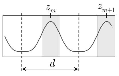
Figure 1: The periodic structure built of quantum wells (the shadowed rectangulars) and the barriers between them. Vertical dashed lines show the boundary of the elementary cell having the property of the mirror symmetry. The smooth line illustrates the modulation of the dielectric function in the structure.

As has been discussed in Ref. Erementchouk et al., 2006, Eqs. (20) and (22) do not yet describe the propagation of the field across an entire elementary cell because they do not include the transfer across the interface between two adjacent elementary cells. The problem is that initial conditions for these solutions are defined at some point inside a given cell, and in order to use them to describe field in a different cell one has to introduce the shift of variables $z\rightarrow z\pm nd$, where $d$ is the period of the structure, and $n$ is the number of periods separating the two cells. After that one could express the functions with the shifted arguments as a linear combination of the original functions, but the most convenient way to describe the transition from one cell to another is to convert our transfer matrices to the basis of plane waves. In this basis the field and its derivative are represented as a superposition of waves propagating along $z$-axis

$$E = E_{+}(z)e^{iqz}+E_{-}(z)e^{-iqz}$$ (24)

$$dE/dz = iqE_{+}(z)e^{iqz}-iqE_{-}(z)e^{-iqz}$$

where $q=\kappa(z_{\pm})$, and can be naturally presented by a two-dimensional vector of the form:

$$\left|E\right\rangle=E_{+}\left|+\right\rangle+E_{-}\left|-\right\rangle,$$ (25)

where

$$\left|+\right\rangle=\begin{pmatrix}1\\ 0\end{pmatrix};\hskip 17.07182pt\left|-\right\rangle=\begin{pmatrix}0\\ 1\end{pmatrix}$$

are the basis vectors of the respective vector space. More detailed description of the plane wave representation can be found in Ref. Erementchouk et al., 2006. The relation between the coefficients $c_{1,2}$ and the amplitudes $E_{\pm}$ is written as

$$\begin{pmatrix}E_{+}\\ E_{-}\end{pmatrix}(z)=M(z)\begin{pmatrix}c_{1}\\ c_{2}\end{pmatrix}(z),$$ (26)

whereErementchouk et al. (2006)

$$M(z)=\frac{1}{2}\begin{pmatrix}h_{1}(z)+\dfrac{h^{\prime}_{1}(z)}{iq}&h_{2}(z)+\dfrac{h^{\prime}_{2}(z)}{iq}\\ h_{1}(z)-\dfrac{h^{\prime}_{1}(z)}{iq}&h_{2}(z)-\dfrac{h^{\prime}_{2}(z)}{iq}\end{pmatrix}.$$ (27)

Applying rule (26) to Eq. (20) we obtain

$$\left|E\right\rangle(z_{+})=T\left|E\right\rangle(z_{-})+\left|v_{m}\right\rangle,$$ (28)

where $T=M(z_{+})\widehat{T}_{h}M^{-1}(z_{-})$ is the transfer matrix through the entire period of the structure in the basis of plane waves. In the case of structures with the symmetrical elementary cell this transfer matrix can be presented asErementchouk et al. (2006)

$$T=\begin{pmatrix}af&(\bar{a}f-a\bar{f})/2\\ (a\bar{f}-f\bar{a})/2&\bar{a}\bar{f}\end{pmatrix},$$ (29)

where

$$\begin{split}a=g_{2},\qquad f=g_{1}-iSg_{2},\\ \bar{a}=g_{2}^{*},\qquad\bar{f}=g_{1}^{*}+iSg_{2}^{*},\end{split}$$ (30)

and

$$\begin{split}g_{1}=\frac{1}{\sqrt{W_{h}}}\left[h_{1}(z_{+})+\frac{h_{1}^{\prime}(z_{+})}{iq}\right],\\ g_{2}=\frac{1}{\sqrt{W_{h}}}\left[iqh_{2}(z_{+})+h_{2}^{\prime}(z_{+})\right].\end{split}$$ (31)

The functions $g_{1,2}(\omega)$, which are obviously not unique, are chosen to make clear the transition to the limiting case of structures with spatially uniform refractive index. In this case choosing $h_{1}(0)=h_{2}^{\prime}(0)=1$ one has $W_{h}=1$ and $g_{1,2}=\exp(iqz_{+})$. The function $S(\omega)=-2\pi\omega^{2}\tilde{\chi}\varphi_{1}^{2}/(qc^{2})$ introduced in Eq. (30) quantifies the interaction of the excitons with light. For the single-pole form of $\chi(\omega)$ it has the form

$$S=\frac{\Gamma_{0}}{\omega-\omega_{0}-\Delta\omega+i\gamma},$$ (32)

where $\Gamma_{0}=2\pi\alpha\omega^{2}\varphi_{1}^{2}/qc^{2}$ is the radiative decay rate. Because of the direct relation between the functions $\tilde{\chi}$ and $S$ (they differ only by a factor slowly changing with frequency) we will for brevity refer to the function $S(\omega)$ as the exciton susceptibility.

The source term (22) in the basis of plane waves takes the form

$$\left|v_{m}\right\rangle=M(z_{+})\begin{pmatrix}\Delta c_{1}\\ \Delta c_{2}\end{pmatrix}=-F_{2}\frac{4\pi\omega^{2}}{c^{2}}\left|a\right\rangle+F_{1}\frac{4\pi\omega^{2}}{c^{2}}\left|s\right\rangle-\frac{2\tilde{\Sigma}Sq}{\varphi_{1}}\left|s\right\rangle,$$ (33)

where

$$\left|a\right\rangle=\frac{1}{2}\begin{pmatrix}g_{1}\\ g^{*}_{1}\end{pmatrix},\qquad\left|s\right\rangle=\frac{1}{2iq}\begin{pmatrix}g_{2}\\ -g^{*}_{2}\end{pmatrix}.$$ (34)

The index $m$ in the notation $\left|v_{m}\right\rangle$ reminds that all the relevant quantities can depend on the number of the well and should be taken for a particular well.

III Radiative boundary conditions and the field emitted by an $m$-th well

Equation (28) expresses the field at the right boundary of the elementary cell in terms of the field given at the left boundary. Formally, it can be understood as the general solution of a Cauchy problem (the general solution of the homogeneous equation plus a particular solution of the inhomogeneous one). The amplitudes $E_{\pm}$ at the left boundary represent two independent parameters that can be chosen to satisfy any particular initial or boundary conditions. To represent a radiation coming out of the structure the field must satisfy radiative boundary conditions that require that outside the structure there must be only outgoing waves. Our objective now is, therefore, to find such $E_{\pm}$ that would satisfy this condition.To this end we consider an $N$ layer structure embedded into an environment with the refractive index $n_{out}$. Scattering of light by the interfaces between the terminal layers of the structure and the surrounding medium is described by the matrices

$$T_{L,R}=\frac{1}{1+\rho_{L,R}}\begin{pmatrix}1&\rho_{L,R}\\ \rho_{L,R}&1\end{pmatrix},$$ (35)

where

$$\rho_{L,R}=\frac{n_{out}\cos\theta_{L,R}-n(z_{L,R})\cos\theta(z_{L,R})}{n_{out}\cos\theta_{L,R}+n(z_{L,R})\cos\theta(z_{L,R})}.$$ (36)

Here $z_{L,R}$ are the coordinates of the left and the right ends of the structure, respectively. The angle of propagation is determined by $\tan\theta(z)=k/\kappa(z)$. The outgoing waves propagate at the angles following from Snell’s law $n_{out}\sin\theta_{L,R}=n(z_{L,R})\sin\theta(z_{L,R})$.

We impose the radiative boundary conditions assuming first that the sources are localized only in the $m$-th layer. We require that in the half-spaces $z<z_{L}$ and $z>z_{R}$, the field outside the structure would have the form of the wave propagating respectively to the left, and to the right. The former field can be described by a basis vector $\left|-\right\rangle$ of the two-dimensional vector space introduced in Eq.(25): $E=E_{-}^{(m)}\left|-\right\rangle$, and the later one is proportional to the other basis vector $\left|+\right\rangle$: $E=E_{+}^{(m)}\left|+\right\rangle$. Using the results of the previous Section we can find the following relation between the fields outside the structure

$$E_{+}^{(m)}\left|+\right\rangle=T_{R}T(N,m+1)\left|v_{m}\right\rangle+E_{-}^{(m)}T_{R}T(N,1)T^{-1}_{L}\left|-\right\rangle,$$ (37)

where

$$T(N,m)=T_{N}\ldots T_{m}$$ (38)

is the transfer matrix through the part of the structure obtained as a product of the transfer matrices through the individual layers. Eq. (37) is obtained by directly applying Eq. (28) to the field at the left end of the structure. This state is transferred through the entire structure in a usual way by a simple multiplication of the transfer matrices describing each period of the structure. This procedure results in the term proportional to the transfer matrix $T(N,1)$. Transfer across the luminescent layer results in an additional contribution as is given by the second term in Eq. (28). After being emitted this field is then transferred across remaining $N-m$ layers yielding the term proportional to $T(N,m+1)$. The matrices $T_{L,R}$ take into account reflection of the radiation at the interface between the terminal layers of the structure, and the outside world.

Multiplication of Eq. (37) from the left by $\left\langle+\right|$ and $\left\langle-\right|$ gives the system of two inhomogeneous equations with respect to $E_{\pm}^{(m)}$. The solution of this system is

$$\begin{split}E_{-}^{(m)}=&-\frac{\left\langle-\right|T_{R}T(N,m+1)\left|v_{m}\right\rangle}{\left\langle-\right|T_{PC}\left|-\right\rangle},\\ E_{+}^{(m)}=&\frac{\left\langle+\right|T_{L}T^{-1}(m,1)\left|v_{m}\right\rangle}{\left\langle-\right|T_{PC}\left|-\right\rangle},\end{split}$$ (39)

where $T_{PC}=T_{R}T(N,1)T_{L}^{-1}$ is the transfer matrix through the whole structure including the interfaces between the terminating layers and the surrounding medium.

Equations (39) can be used to derive expression for Green’s function defined as a function relating the radiated field with the source. We can write the amplitudes of the waves outside in the form

$$E_{\pm}^{(m)}=\mathcal{G}_{\pm}^{(s)}(m)\left(F_{1}-\tilde{\Sigma}\varphi_{1}\tilde{\chi}\right)\frac{4\pi\omega^{2}}{c^{2}}+\mathcal{G}_{\pm}^{(a)}(m)\left(F_{2}-\tilde{\Sigma}\varphi_{2}\tilde{\chi}\right)\frac{4\pi\omega^{2}}{c^{2}},$$ (40)

where

$$\mathcal{G}_{-}^{(s,a)}(m)=\mp t_{N}\left\langle-\right|T_{R}T(N,m+1)\left|s,a\right\rangle,\qquad\mathcal{G}_{+}^{(s,a)}(m)=\pm t_{N}\left\langle+\right|T_{L}T^{-1}(m,1)\left|s,a\right\rangle.$$ (41)

Here we take into account the definition of the transmission coefficient through the whole structure $t_{N}$ in terms of the transfer matrix $t_{N}=\left\langle-\right|T_{PC}\left|-\right\rangle^{-1}$. We would like to emphasize that these expressions are valid with the vectors $\left|s\right\rangle$ and $\left|a\right\rangle$ defined by Eqs. (34) even for non-symmetrical structures where $\left|s\right\rangle$ and $\left|a\right\rangle$ do not imply symmetrical properties.

Equation (39) can also be used to find the distribution of the field created by the source inside the structure. This can be achieved in two different ways. One can start, for instance, with field $E^{(-)}_{m}\left|-\right\rangle$ on the left-hand side of the structure and propagate it across using transfer-matrices. When a luminescent layer is reached, Eq. 28 should be employed to describe transfer across it. Alternatively, one can propagate $E^{(-)}_{m}\left|-\right\rangle$ to find field in the elementary cells to the left of the luminescent layer, and propagate $E^{(+)}_{m}\left|+\right\rangle$ from the right to determine field in the cells to the right of it.

We would also like to add that Eq. (40) can be used also for studying the directional and in-plane distributions of the field. For example, the standard problem of a point source can also be considered since the in-plane distribution of the source is taken into account by 2D Fourier transform (8).

Equation (40) shows that the field outside is determined by two parameters found as convolutions of the sources with the functions $h_{1,2}(z)$. As has been demonstrated in Ref. Erementchouk et al., 2006, these functions provide complete description of photonic modes of a respective infinite system. From this perspective the result of Eq. (40) might seem expected. Indeed, it looks somewhat similar to a standard construction where the response is determined by a superposition of modes with amplitudes determined by the projections of the excitation onto the modes. This analogy, however, is misleading for the case under consideration. There are several important features distinguishing Eq. (40) from the standard Green’s function formalism. First, as has been noted, the functions $h_{1,2}(z)$ do not have to coincide with photonic modes even locally (inside a particular elementary cell). Second, Eq. (40) is written for a finite structure when the applicability of the modes of an infinite structure can not be trivially justified. Third, Eq. (40) does not require restrictive properties of the operators governing the propagation of light (say, hermicity) and, in particular, with slight modifications remains valid in the presence of losses in the dielectric ($\mathrm{Im}[n(z)]\neq 0$) while in this case even the notion of the projection has to be carefully examined.

Below we will concentrate mostly on the case when the elements of the structure and the structure itself have the mirror symmetry. As a result, the index mismatch between the surrounding medium and the terminal layers is the same for both boundaries, so that one has $T_{L}=T_{R}=T_{\rho}$. It is interesting to note that in such structures the solutions given by Eq. (40) do not necessarily guarantee the symmetry of the radiation emitted to the left and to the right of the structure. For such symmetry to take place one has to prove that

$$E_{-}^{(N-m+1)}=E_{+}^{(m)}.$$ (42)

This relation can indeed be proven but only in the case when both the structure and the sources are symmetrical with respect to the centers of the elementary cells. While the exciton related resonance source term does have the required symmetry, the non-resonance contribution is not necessarily symmetric if both $F_{1,2}\neq 0$ (see Eq. (33) and Eq. (7)). If this is indeed the case than radiation emitted to the right would not have the same characteristics as radiation emitted to the left. When $F_{2}\equiv 0$, however, Eq. (42) can be proven with the help of relation $T^{-1}\left|s\right\rangle=-\sigma_{x}\left|s\right\rangle$, where $T$ is defined in Eq. (29), and $\sigma_{x}$ is the standard Pauli matrix.

As follows from Eq. (40) the field radiated due to the exciton recombination has, as expected, the resonant character. Thus, in resonant PCs the recombination determines the spectrum of the radiated field at frequencies close to $\omega_{0}$, while the non-resonant sources specified by $F(z)$ are responsible for the background component characterized by a relatively smooth frequency dependence. This contribution may become important farther away from the exciton frequency. For the problem of the exciton luminescence in the resonant PCs these non-resonant sources are not important and, therefore, below we assume that the only source of radiation is the exciton recombination and neglect the non-resonant contribution. The expression for the radiated field essentially simplifies in this case and takes the form

$$E_{\pm}^{(m)}=-\mathcal{G}_{\pm}(m)\Sigma_{m}\frac{2S_{m}q}{{\varphi_{m}}_{1}},$$ (43)

where we explicitly show the dependence of the source on the number of the layer and

$$\mathcal{G}_{\pm}(m)=\pm t_{N}\left\langle\pm\right|T_{\mp}(m)T_{\rho}\left|s\right\rangle.$$ (44)

Here we have taken into account that $\tilde{\Sigma}_{m}=\Sigma_{m}$ when $F\equiv 0$ and have dropped the superscript $(s)$ since the only relevant Green’s function in this case is $\mathcal{G}_{\pm}^{(s)}(m)$. We have also introduced partial transfer matrices $T_{-}(m)=T_{\rho}T^{-1}(m,1)T_{\rho}^{-1}$ and $T_{+}(m)=T_{\rho}T(N,m+1)T_{\rho}^{-1}$, which have the property $T_{-}^{-1}(m)T_{+}(m)=T_{PC}$.

IV The luminescence spectrum of resonant photonic crystals

IV.1 Quasi-classical approach to luminescence

In this section we will apply general results of previous sections to the problem of the luminescence spectrum of multiple-quantum-well based resonant photonic crystals. Luminescence is one of the manifestations of spontaneous emission, and as such is a purely quantum electrodynamic phenomenon. At the same time, the non-coherent radiation produced due to luminescence in many situations can still be described as classical electromagnetic field with randomly changing amplitude and phase. The average value of such a field is equal to zero, while its variance, defined as $\langle E^{2}({\bf r})\rangle$, is identified with intensity, where angular brackets $\langle\cdots\rangle$ symbolize averaging over appropriately defined distribution function. Such a quasi-classical approach to spontaneous emission has been used previously in a great number of different situations. Just as a small sample of papers dealing with applications of classical electrodynamics to the problem of spontaneous emission we can refer to Ref. Morawitz, 1969; Dowling and Bowden, 1992; Stanley et al., 1996; Dodd, 1997; Xu et al., 2000.

One of the methods of reproduction of non-coherent classical field is a Langevin-like approach, in which the polarization sources appearing in macroscopical Maxwell equations (1) are considered as random functions of time and coordinates whose statistical characteristics should be determined either from experiment or from fully quantum microscopical theory. In what follows we will neglect the non-resonant contribution to polarization $F$, and characterize statistical properties of the resonant source function $\Sigma_{m}(\mathbf{\rho},t)$ by a correlation function

$$\langle\Sigma_{i,m}(\mathbf{\rho},t)\Sigma_{j,l}(\mathbf{\rho}^{\prime},t^{\prime})\rangle=\delta_{ij}\delta_{ml}K_{\Sigma}\left(\mathbf{\rho}-\mathbf{\rho^{\prime}},t-t^{\prime}\right),$$ (45)

where $\langle\cdots\rangle$ signifies statistical averaging over various realizations of the non-coherent exciton polarization, indexes $i$ and $j$ designate Cartesian coordinates in the $(x,y)$-plane, and $m$ and $l$ are well numbers. Equation (46) implies that the fluctuations of the non-coherent exciton polarization are (i) statistically uniform in time and space, (ii) direction of the non-coherent polarization is distributed isotropically in the plane of the structure, with various components of the polarization vector independent of each other, and (iii) source functions in different wells do not correlate with each other.

This correlation function can only be found from a microscopical theory of electron-hole relaxation processes. An example of such a theory, which provide a more quantitative justification for our phenomenological approach and shows relation of this correlation function to microscopic characteristics of quantum wells, is presented in Appendix. These calculations demonstrate that all three assumptions regarding properties of the source correlations are justified. The most important of them is the assumption of independence of the source functions in different wells. We would like to emphasize here that this assumption does not mean that we neglect radiative coupling between wells. As it is explained in Appendix the source term $\Sigma_{m}(\mathbf{\rho},t)$ is determined by excitons populating non-radiative states so that the electromagnetic field associated with them decays exponentially outside of the wells and does not contribute to the radiative coupling. This coupling is described by the common radiative field $E$ which is created by and act on all quantum wells in the system as it was explained in previous section II. It is interesting to note that Maxwell equation (1) describes this coupling even though the average value of the non-coherent field is equal to zero. The correlation function for the fourier transformed source function $\Sigma_{m}(\omega,{\bf k})$ is given by spectral density $\Xi_{m}(\omega,k)$ defined as

$$\langle\Sigma_{m}(\mathbf{k},\omega)\Sigma_{l}(\mathbf{k}^{\prime},\omega^{\prime})\rangle=\Xi_{m}(\omega,k)\delta(\omega-\omega^{\prime})\delta(\mathbf{k}-\mathbf{k}^{\prime})\delta_{ml}$$ (46)

which is a Fourier transform of the time-position correlation function given in Eq.(45).

The field created by such source is characterized by a spectral intensity $\mathcal{I}(\mathbf{k},\omega)$ defined as

$$\langle E(\mathbf{k}_{1},\omega_{1})E(\mathbf{k}_{2},\omega_{2})\rangle=\mathcal{I}(\mathbf{k}_{1},\omega_{1})\delta(\mathbf{k}_{1}-\mathbf{k}_{2})\delta(\mathbf{\omega}_{1}-\mathbf{\omega}_{2}).$$ (47)

Applying Eq. (46) to this equation we find the spectral intensity of radiation emitted by the entire structure in the form

$$\mathcal{I}_{\pm}(\omega,k)=4\,\sum_{m}\Xi_{m}(\omega,k)|\mathcal{G}_{\pm}(m;\omega,k)|^{2}\left|\frac{qS_{m}(\omega,k)}{{\varphi_{m}}_{1}}\right|^{2}.$$ (48)

which implies that the field emitted by different wells adds in a non-coherent way. This general expression allows analyzing both the frequency and the directional dependence of the luminescence spectrum. In this work we restrict our consideration to the waves emitted along the growth direction of the structure (i.e. $k=0$). The directional distribution of the radiation will be studied elsewhere.

Equation (48) shows that the form of the luminescence spectrum is determined by several factors with different frequency dependencies. The exciton susceptibility, $S(\omega)$ for instance, strongly reduces the luminescence far away from the exciton frequency $\omega_{0}$. The spectral density $\Xi(\omega)$ is expected to show a weak frequency dependence at the scale of the width of the polariton stop-band. The factor $|\mathcal{G}(m;\omega,k)|^{2}$, according to Eq. (44), is the product of two terms. One is the transmission coefficient $t_{N}$, which may have strong frequency dependence following the singularities at the eigenfrequencies of the quasi-modes of the structure. These singularities determine the fine structure of the luminescence spectrum. The second term is responsible for the variations in the luminescence intensity at a much larger scale. Equation (48) can be used to analyze spectra of luminescence of various types of MQW structures. Several examples are presented in the subsequent parts of this section.

IV.2 The luminescence spectrum of finite periodic structures

IV.2.1 General expression for intensity of emission

We first apply our general results to the case structures built of identical layers, so that ${\varphi_{m}}_{1}=\varphi_{1}$ and $S_{m}=S$, i.e. all quantum wells are characterized by the same exciton frequency $\omega_{0}$. We would like to note that in order to have the structure with the mirror symmetry it must contain an integer number of the elementary cells. This means, in particular, that the terminating layers are half-barriers. As has been noticed, in this case the luminescence spectrum is the same at the both sides of the structure. For the concreteness, we will consider the field radiated to the right (i.e. $E_{+}$).

In the symmetric case we can perform the summation over the quantum wells using the fact that all partial transfer matrices posses the mirror symmetry and can be presented in the formErementchouk et al. (2005)

$$T(\theta,\beta)=\begin{pmatrix}\cos\theta-i\sin\theta\cosh\beta&-i\sin\theta\sinh\beta\\ i\sin\theta\sinh\beta&\cos\theta+i\sin\theta\cosh\beta\end{pmatrix},$$ (49)

where

$$\cos\theta=\frac{1}{2}(af+\bar{a}\bar{f}),\qquad\tanh\beta=\frac{\bar{a}f-a\bar{f}}{af-\bar{a}\bar{f}}.$$ (50)

The parameter $\theta$ determines the polariton spectrum of an infinite structure and is defined as $\theta=Kd$, where $K$ is the polariton Bloch wave-number.

The representation (49) is convenient because all $T_{-}(m)$ are characterized by the same $\beta$, while the spectral parameter of $T_{-}(m)$ is merely $-m\theta$. Thus, $T_{-}(m)$ can be written as

$$\begin{split}T_{-}(m)=&\,e^{im\theta}U(\beta/2)\left|+\right\rangle\left\langle+\right|U^{-1}(\beta/2)\\ &+e^{-im\theta}U(\beta/2)\left|-\right\rangle\left\langle-\right|U^{-1}(\beta/2),\end{split}$$ (51)

where $U(\beta/2)\equiv T_{\rho}T_{H}(\beta/2)$, and $T_{H}$ is a matrix describing a hyperbolic rotation with a dilation

$$T_{H}(\beta)=e^{\beta}\begin{pmatrix}\cosh\beta&-\sinh\beta\\ -\sinh\beta&\cosh\beta\end{pmatrix}.$$ (52)

Matrix $T_{\rho}$ takes into account reflection and transmission at the external boundaries of the system.

Using Eq. (51) one can find

$$\frac{4q^{2}}{|t_{N}|^{2}}\sum_{m}\left|\mathcal{G}_{+}(m)\right|^{2}=\frac{\sinh N\theta^{\prime\prime}}{\sinh\theta^{\prime\prime}}\left[|A|^{2}e^{-(N+1)\theta^{\prime\prime}}+|B|^{2}e^{(N+1)\theta^{\prime\prime}}\right]+\frac{\sin N\theta^{\prime}}{\sin\theta^{\prime}}\left[AB^{*}e^{i\theta^{\prime}(N+1)}+A^{*}Be^{-i\theta^{\prime}(N+1)}\right],$$ (53)

where we have introduced real and imaginary parts of the dimensionless Bloch number, $\theta$: $\theta=\theta^{\prime}+i\theta^{\prime\prime}$ and parameters

$$\begin{split}A=&\frac{1}{1+\rho}\left[(g_{2}-\rho g^{*}_{2})\cosh^{2}(\beta/2)-\frac{1}{2}(g_{2}^{*}-\rho g_{2})\sinh\beta\right]\\ B=-&\frac{1}{1+\rho}\left[(g_{2}-\rho g^{*}_{2})\sinh^{2}(\beta/2)-\frac{1}{2}(g_{2}^{*}-\rho g_{2})\sinh\beta\right].\end{split}$$ (54)

For the purposes of numerical calculations instead of direct calculations of the parameter $\beta$ it is more convenient to multiply both parts of Eqs. (54) by $\sin\theta$ and, then, use Eq. (49) to establish direct relation of corresponding terms with the elements of the transfer matrix through the period of the structure.

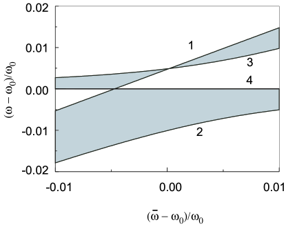
Figure 2: (color online) Evolution of polariton band boundaries with detuning of the structure with piecewise modulation of the refractive index from exact Bragg condition. The horizontal axis describes the detuning in terms of parameter $\bar{\omega}-\omega_{0}$, where $\bar{\omega}=\pi c/(n_{w}d_{w}+n_{b}d_{b})$, $n_{w}$, $n_{b}$, $d_{w}$, $d_{b}$ and refractive indexes and thicknesses of well and barrier layers respectively. The vertical axis shows a relative difference between frequency $\omega$, and exciton frequency $\omega_{0}$.

While Eq. (53) describes luminescence of a periodic MQW structure with an arbitrary period, we shall focus our attention to the most interesting cases of Bragg and near-Bragg structures,Ivchenko (1991); Ivchenko et al. (1994) in which effects of periodic modulation of the refractive index and light-exciton coupling are most pronounced. As we already mentioned in Introduction the period, $d$, of such structures satisfies a special resonance condition $\omega_{0}=\omega_{B}(d)$, where the exact value of the resonant frequency $\omega_{B}$ in systems with periodically modulated refractive index depends not only on the period of the structure, but also on details of the modulation.Ivchenko et al. (2004); Erementchouk et al. (2006) For concreteness we will assume that the dielectric function reaches its maximum value at the quantum well and monotonously decreases towards the boundaries of the elementary cell. In this case the Bragg resonance takes place when the exciton frequency coincides with the high-frequency boundary of the photonic band gap, $\Omega_{+}$. Since the details of the emission spectrum are determined to a large extent by the electromagnetic band structure of the systems under consideration, it is useful to remind the main features of this structure, which was analyzed in details in a number of papers.Ivchenko et al. (1994); Ivchenko (1991); Deych and Lisyansky (2000); Ivchenko et al. (2004); Erementchouk et al. (2006) Fig. 2 shows the dependence of band boundaries of MQW structure upon its period, where shaded regions correspond to polariton stop-bands. One can see that at a certain value of $\bar{\omega}=\pi c/(n_{w}d_{w}+n_{b}d_{b})$, where $n_{w}$, $n_{b}$, $d_{w}$, $d_{b}$ and refractive indexes and thicknesses of well and barrier layers respectively, two stop-bands connect at the exciton frequency $\omega_{0}$ forming a single wide band-gap. This is the point of the Bragg resonance, when exciton frequency falls inside a stop-band of the spectrum, whose width can be much larger than the width of the exciton resonance. (The second occurrence of a single band situation at larger values of $\bar{\omega}$ results from collapse of one of the gaps, and is a result of random degeneracy between two exciton polariton branches.) Spectrum of structures only slightly detuned from the Bragg condition (we will use term quasi-Bragg for such structures), is characterized by emergence of a propagating band between the two stop-band. The exciton frequency in this case belongs to the boundary of the propagating band, which is situated asymmetrically with respect to the outer band boundaries: for negative detunings $\omega_{0}$ is closer to the upper boundary, while for positive detuning the lower polariton branch eventually moves closer to it.

Equation( 53) demonstrates how the polariton band structure affects the luminescence of the system under consideration. One can see from this equation that the structure of the spectrum is characterized by two scales of frequencies. On a smaller scale the modulations of the intensity of emission are determined by $|t_{N}|^{2}$ term in Eq. (53), whose maxima correspond to the real parts of the polariton eigenfrequencies. The modulation of intensity on this scale depends on the number of periods in the structure and occurs over frequency intervals of the order of $v_{g}/(dN)$, where $v_{g}$ is the group velocity of the polariton excitations and $d$ is the period of the structure. The polariton band structure affects the luminescence on a much larger spectral scale through the combination of the exciton susceptibility $S(\omega)$ and the imaginary part of the polariton Bloch number presented by parameter $\theta^{{}^{\prime\prime}}$.

Homogeneous and inhomogeneous broadenings significantly effect the short-scale modulations of the luminescence allowing for their observation only in high quality samples at very low temperatures. At higher temperatures the long scale variations of intensity, which depend significantly on relations between $\omega_{0}$ and $\omega_{B}$, become predominant. In the case of Bragg structures, when $\omega_{0}$ is very close to $\omega_{B}$, Eq. (53) predicts that the luminescence spectrum is mostly concentrated outside of the polariton stop-band near the edges of the bands of the exciton polaritons. Indeed, at frequencies inside the forbidden gap the contribution to $\mathcal{I}(\omega)$ of the exponentially large terms in the right-hand-side of Eq. (53) is canceled by the exponentially small transmission at these frequencies. As a result, only wells within the attenuation length from the boundaries contribute to the radiated field. Besides at frequencies far away from the $\omega_{0}$ the luminescence is subdued by the smallness of the exciton susceptibility. These qualitative arguments can be supported by direct calculation of the emission intensity in the neighborhood of the band edges, where Eq. (53) can be simplified. In this spectral region we can represent the spectral parameter as $\theta=\pi+i\epsilon$ and assume that $\epsilon$ is sufficiently small, so that $N|\epsilon|\ll 1$. Obviously, this approximation covers a substantial interval of frequencies only for not very long structures, but it is quite sufficient for a qualitative analysis of realistic structures.

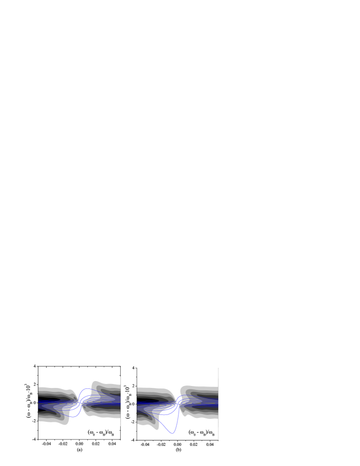
Figure 3: (color online) The luminescence spectrum in comparison with a polariton band structure is shown for quasi-Bragg structures consisting of $60$ layers near the boundary of the first Brillouin zone. Smooth filling corresponds to the luminescence calculated using $\Xi=1$. The lines are the contour plot of $\theta^{\prime\prime}$, where the outermost curve correspond to its smallest value. Frequency changes along the vertical axis, while, the horizontal one presents detuning from the Bragg resonance. (a) Pure MQW structure with parameters typical for Al_xGa_1-xAs/GaAs structures: $\Gamma_{0}=75$ $\mu$eV, $\omega_{0}=1.489$ eV, $\gamma=300$ $\mu$eV. (b) An example of MQW based photonic crystal. The exciton related parameters are the same as in (a). The modulation of the index of refraction is taken to be $n(z)=3.4+0.1\cos^{20}(\pi z/2d)$.

Expending Eq. (48) in a power series with respect to the small parameter $\epsilon N$, we can approximate it by the following simple expression:

$$\mathcal{I}(\omega)\approx N\Xi(\omega)|t_{N}|^{2}\left|\frac{S(\omega)}{\varphi_{1}}\right|^{2}\frac{h^{2}_{2}q^{2}}{W_{h}}.$$ (55)

An important result immediately demonstrated by this equation is a linear increase of the intensity of the emission with the number of quantum wells. This is an expected behavior because of the transparency of the structure at these frequencies and the independence of the contributions of different wells to the emitted light. Another important conclusion following from Eq. (55) is a relative weakness of the luminescence of the Bragg structures. The cause of the decrease in the emission is related to the presence of a broad polariton stop-band in such structures whose width, $\Delta$, given by expression $\Delta=\sqrt{2\Gamma_{0}\omega_{0}/\pi}$, is much larger than the width of the exciton susceptibility $S(\omega)$ determined by non-radiative decay, $\gamma$. In the interior of the stop-band the luminescence is suppressed by small transmissivity of the structure in the vicinity of the exciton resonance, while at the edges of the stop-band it is reduced by the factor of $\Gamma_{0}/\omega_{0}\ll 1$ because of the separation of the band boundaries from the exciton frequency. The found decrease in luminescence for Bragg structures is equivalent to the so called sub-radiance effect obtained in Ref. Schäfer et al., 2006 on the basis on fully quantum calculations. We demonstrate here that this effect has a purely classical origin and is caused by formation of polariton stop-band in Bragg MQW systems.

Detuning from the Bragg resonance opens up a transparency window inside the stop-band with exciton frequency coinciding with one of the band boundaries (Fig.2). On the base of the same arguments as above one can expect that the emission spectrum is characterized by two maxima: the stronger one in the vicinity of the boundary of the propagating band adjacent to $\omega_{0}$, and the second, weaker, maximum at the boundary of the outer polariton band, which is closer to the exciton frequency. The second outer boundary of the polariton band is so remote from the exciton frequency that its contribution to emission can be neglected. Numerical calculations carried out with the exact form of $\mathcal{I}(\omega)$ confirm these conclusions. The results of these calculations are presented in Fig. 3, where we show the dependence of the intensity upon frequency and the period of the structure. The intensity is shown by the shading on the graphs — the darker shading corresponds to higher emission. In order to facilitate a better understanding of the role of the refractive index contrast we simulated two types of structures: one with a realistic changes in the refractive index between wells and barriers, and the other, in which refractive index was assumed constant throughout a structure. The latter structures are often called optic lattices because all the modifications in their optical properties come from the radiative coupling between quantum well excitons. It is interesting to see a significant difference between the luminescence spectra of MQW optical lattices and MQW based photonic crystals. The latter is asymmetric with respect to the point of the Bragg resonance, while the former shows complete symmetry. This feature is clearly related to the asymmetrical structure of the polariton band gap in structures with modulated refraction index.Erementchouk et al. (2006)

Figure 4: The fine structure of the luminescence spectrum. The parameters of the structures are the same as in Fig. 3 except $\gamma=30$ $\mu$eV. For better visibility the shadow intensity is chosen according to the log-scale. (a) The MQW structure with a homogeneous dielectric function. (b) The MQW based photonic crystal.

In order to emphasize the relationship between the luminescence spectrum and polariton band structure, the spectrum in this figure is presented together with the polariton stop band. The latter is shown with the help of level curves of the imaginary part of the dimensionless Bloch vector $\theta^{\prime\prime}$. In an ideal system without any broadenings, $\theta^{\prime\prime}$ would have been zero everywhere outside of the stop-band. In real systems, of course, $\theta^{\prime\prime}$ is not zero everywhere because of the exciton broadening. This makes the notion of the stop-band not very well defined, and, in particular, the edges of the gap can not be determined unambiguously. However, at the frequency, which would correspond to the band edge in a system without broadening, the imaginary part of the polariton Bloch wave-number drastically increases. This increase can be traced on the level curves of $\theta^{\prime\prime}$ in Fig. 3, where outer curves correspond to the smallest value of $\theta^{\prime\prime}$. It is seen that the maxima of the luminescence spectrum approximately follow these lines when the relation between the the exciton frequency and the period of the structure changes. The exact position of the maxima is determined by an interplay between a smaller value of $\theta^{\prime\prime}$ (and, hence, a higher transmission) and a smaller distance from the exciton frequency (a higher value of $S(\omega)$). Comparing the spectrum shown in Fig. 3 with the band structure shown in Fig. 2 one has to notice the different frequency scales of these figures. The frequency region covered in Fig. 3 includes only the small transparency window around the exciton frequency and only the closest to it outer polariton band.

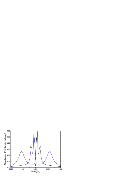
Figure 5: (color online) Fine structure of the PL spectra for the 100 wells MQW structures with different periods. Curves 1, 2 and 3 are calculated for the period respectively smaller, equal, and larger than the Bragg resonance value. The indexes of refraction of wells and barriers in this calculation were assumed equal to each other.

For sufficiently smaller value of the exciton broadening the fine structure becomes clearly visible as is seen in Fig. 4. As we mentioned above the maxima of the luminescence forming this fine structure result from the periodic dependence of the transmission on frequency. These maxima appear as the characteristic scars on the spectrum presented in this figure. More clear representation of these features of the luminescence spectrum can be given by direct plotting of the intensity as function of frequency for different values of the de-tuning of the structure from the Bragg resonance, as shown in Fig. 5, which was obtained neglecting the modulation of the refractive index.

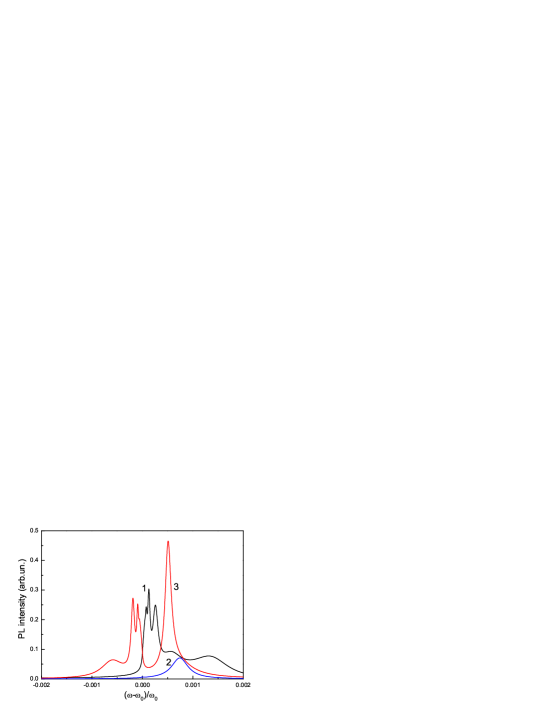
Figure 6: (color online)The same spectra as in Fig. 5 but with cladding layer of thickness $d_{c}=d_{b}+d_{w}/2$

IV.2.2 Comparison with experiment and the role of inhomogeneous broadening

Comparing our calculations with experimentally observed spectra,Hubner et al. (1999); Mintsev et al. (2002) one should take a few considerations into account. First of all, the direct quantitative comparison is rather difficult because the experimental spectra are influenced by details of the entire experimental sample, and not just by its MQW part. For instance, the details of the cladding layer can significantly influence the observed luminescence spectrum. In order to illustrate this point we used the general formulas derived in the paper to calculate the emission intensity in the presence of the cladding layer. The results of these calculations are shown in Fig. 6, where one can notice significant changes introduced by the cladding layer to the spectra. Second, in photoluminescence experiments with long MQW structures the intensity of pump radiation is not uniform along the structure, which results in different source functions for different wells. This circumstance also affects observed spectra as can be demonstrated by direct computations using general formulas obtained

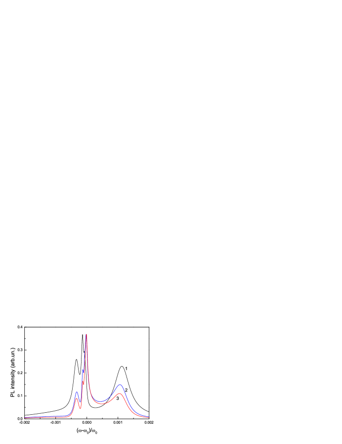
Figure 7: (color online) The luminescence spectrum of the almost Bragg $100$ layers structure with exponentially decaying source term characterized by the decay rate $\alpha$: curve 1 corresponds to $\alpha=0$, curve 2 to $\alpha=0.1$ and curve 3 represents $\alpha=0.2$

in this Section. To this end we assumed that the source function, $\Xi_{m}(\omega)$, which appears in Eq. (48) can be presented as an exponentially decreasing function of the well number, $m$: $\Xi_{m}(\omega)\propto\exp({-\alpha md})$, where parameter $\alpha$ represents an inverse attenuation length of the pump. Using this representation for the source function in Eq. (48) we numerically calculated emission intensity with different values of parameter $\alpha$. The results of these calculations are shown in Fig. 7, where luminescence spectra with $\alpha=0$ and $\alpha=0.2$ are compared. This figure clearly demonstrates that inhomogeneity of the source function can have a significant impact on the observed spectra.

Having in mind mentioned circumstances, we will not attempt to quantitatively reproduce experimental spectra, focusing instead on the most significant features, which most likely have intrinsic origin. Comparing experimental results of Refs. Hubner et al., 1999 and Mintsev et al., 2002, one can notice that despite of quantitative difference between these two experimental spectra, they share one common feature, which is, at the same time is in a striking contrast with results of our calculations. According to our predictions, the luminescence must be most intense in the vicinity of the exciton frequency, while the experiments show that out of two most pronounced maxima of the emission, the one, which is farther away from $\omega_{0}$ is brighter.

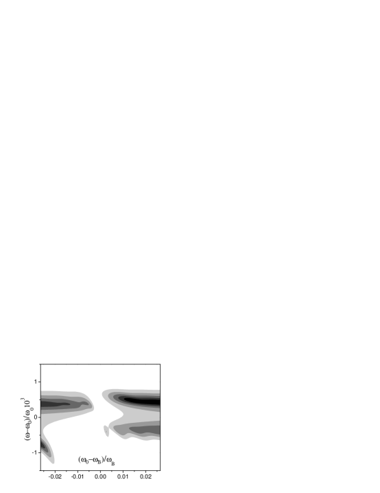
Figure 8: The same spectra as in Fig. 3a, but with inhomogeneous broadening taken into account within the effective medium approximation. The parameter of inhomogeneous broadening was chosen to be equal to $\sigma=200\hskip 2.0pt\mu eV$.

Figure 9: Cross-sections of the intensity profile shown in Fig. 8 for three different values of detuning from exact Bragg resonance.

One probable reason for this discrepancy is the inhomogeneous broadening of excitons, which has not yet been taken into account in our calculations. In this work we include effects due to the inhomogeneous broadening into consideration using a simple model of effective medium.Andreani et al. (1998); Deych et al. (2004) Within this model one neglects spatial dispersion of excitons and assumes that inhomogeneous broadening is caused by spatial fluctuations of exciton frequency $\omega_{0}$. It is further assumed that these fluctuations can approximately be taken into account by replacing exciton susceptibility, Eq. (3), in all relevant equations, with its average value

$$\chi(\omega)_{eff}=\int{\frac{\alpha}{z-\omega-i\gamma}\rho(z)dz},$$ (56)

where $\rho(z)$ is a distribution function of exciton frequencies. In the case of a not very strong inhomogeneous broadening this function can be approximated by a Gaussian:

$$\rho(z)=\frac{1}{\sqrt{\pi}\sigma}\exp{\left[-\displaystyle{\frac{\left(z-\overline{\omega}_{0}\right)^{2}}{\sigma^{2}}}\right]},$$ (57)

where $\overline{\omega}_{0}$ is an average exciton frequency, and its r.m.s. value, $\sigma$ determines the width of the distribution. This model of the inhomogeneous broadening was first introduced in Ref. Andreani et al., 1998 on heuristic basis for calculations of reflection and transmission spectra of MQW structures, and later more rigorously justified in Ref. Deych et al., 2004. While derivation of this model carried out in Ref.Deych et al., 2004 cannot be directly applied to the luminescence problem, we still believe on the ground of physical arguments similar to those put forward in Ref. Andreani et al., 1998, that the effective medium approach can give qualitatively accurate description of the role of inhomogeneous broadening in luminescence spectra, at least, for emission in directions close to normal. Indeed, light emitted by quantum well excitons in the close to normal direction leaves the quantum well without moving significantly in the in-plane direction, and thus without experiencing significant scattering due to in-plane disorder. Accordingly, the main effects of the in-plane disorder in this case is that excitons localized in different regions of the sample emit light at different frequencies. A probe with a sufficiently large aperture (a typical situation in luminescence experiments unless one deals with microluminescent spectra) would collect light emitted by all these excitons, effectively averaging out their susceptibility.

The result of numerical computation of emission spectra with Eq. (56) for exciton susceptibility are presented in Figs. (8) and (9). The first of these figures show that taking into account the inhomogeneous broadening resulted in spectral redistribution of the emission intensity from peaks closer to the central exciton frequency to those that are farther away from it. The latter are now brighter than the former in a qualitative agreement with experimental spectra. This point is demonstrated even more clear in the second of these figures, which shows emission spectra for three values of detuning from Bragg resonance. Qualitatively this affect can be understood by noticing that by averaging the exciton susceptibility we essentially smoothed its resonance dependence on the frequency reducing, therefore, effect of decreasing susceptibility on the emission intensity. In this situation the intensities of luminescence peaks are determined by an interplay between affects due susceptibility and transmissivity of the structure. These calculations show that inhomogeneous broadening can be in principle responsible for observed luminescent spectra, while it is clear that a quantitative agreement with experiment would require more rigorous treatment of inhomogeneous broadening as well as taking into account such effects as inhomogeneity of pump and cladding layers.

IV.3 The luminescence spectrum of structures with defects

One of the main reasons for the interest to resonance photonic crystals derives from possibilities to manipulate their optical properties through modification of their structure. One of the possible approaches includes intentional violation of the periodicity of the PCs by introducing one or several defects. In one-dimensional structures such defects are layers with different characteristics. Depending upon which parameters of the defect layer are modified one can have a variety of defect structures. Effects of such defects on reflection/transmission properties have been studied for both regularStanley et al. (1993); Liu (1997); Figotin and Gorentsveig (1998); Ozaki et al. (2004) and resonant photonic crystals.Deych et al. (1987); Citrin (1995); Deych and Lisyansky (1998); Deych et al. (2000, 2004); Erementchouk et al. (2005); Deych et al. (2003) In the particular case of Bragg MQW structures it was demonstrated, for instance, that by using different types of defects one can engineer structures with a wide variety of optical spectra.Deych et al. (1987) It is clear that defects will also substantially affect luminescence properties of the Bragg structures. Despite the obvious interest of this issue for applications, it has not yet been addressed, and in this paper we present the initial analysis of this problem for one particular type of the defect structure.

The role of the defects on the luminescence spectrum of Bragg MQW structures is two-fold. Firstly, the defects affect the emission of the regular part of the structure caused by the modification of the transmission spectrum, $t_{N}$, of the structure. Secondly, the defect layers, depending on their structure, can contribute their own luminescence to the total spectrum. It should be noted, however, that the second contribution is expected to be small because of the much smaller number of the defect layers compared to the total number of the periods in the structure.

In this paper we will illustrate a possibility to modify luminescence of Bragg MQW structures with the help of structure manipulation by considering one particular case of a defect structure. We will consider a $(2N+1)$-layer multiple quantum well structure, in which the first and the last $N$ layers have a fixed width $w$, while $(N+1)$-th layer at the middle does not contain a quantum well and has a width $d$. To simplify our analysis we will neglect the refractive index contrast between well and barriers in the structure. This type of defect can be described as a cavity, in which parts of the structure to the right and to the left of the defect layer are identified as mirrors. Transmission and reflection properties of this structure in the region of the stop-band have been studied in Ref. Deych et al., 1987 in the limit of very long structures. Here we will consider more realistic case of relatively short structures, and will analyze the manifestations of this defect in luminescence.

The transmission properties of the structure are described by the transfer matrix

$$T=T_{w}^{N}T_{d}T_{w}^{N},$$ (58)

where $T_{w}$ and $T_{d}$ are transfer-matrices through layers with and without quantum wells, respectively,

$$T_{w}=\begin{pmatrix}e^{i\phi_{w}}(1-iS)&-iS\\ iS&e^{-i\phi_{w}}(1+iS)\end{pmatrix},\qquad T_{b}=\begin{pmatrix}e^{i\phi_{d}}&0\\ 0&e^{-i\phi_{d}}\end{pmatrix},$$ (59)

with $\phi_{w}=kw$ and $\phi_{d}=kd$.

The luminescence spectrum can be calculated using general expression (48). As has been noted, the strongest effect on the luminescence spectrum can be expected due to the modification of the transmission by the defect layer. We consider this effect for the case when it is most pronounced, i.e. when MQW parts of the structure satisfy the Bragg condition, $\phi_{w}(\omega_{0})=\pi$. In $N$-layer MQW structures without the defect the transmission in this case has a deep with the width $\sim N\Gamma_{0}$ centered at the exciton frequency, $\omega_{0}$. The resonant tunneling induced by the defect mode results in the appearance of the resonant transparency that, in turn, leads to resonant grow of the luminescence at the respective frequencies. In order to provide a qualitative description of this effect it is more convenient to work with reflection $r=-T_{21}/T_{22}$ and consider its resonance drop caused by the defect layer. Using the representation (49) for the transfer matrices surrounding the defect layer, one can find for not too long structures

$$T_{21}\propto\cos\phi_{d}+N\sin\phi_{d}(\sin\phi_{w}-S\cos\phi_{w}).$$ (60)

Taking into account that $T_{22}$ does not have a significant frequency dependence, we can assume that the minimum of the reflection, $\omega_{min}$, occurs at the same frequency as the minimum of $T_{21}$. Neglecting the homogeneous width of the exciton resonance compared to the width of the stop-band $\Delta_{\Gamma}$, we can present an equation determining $\omega_{min}$ in the form:

$$\frac{\omega_{min}}{\omega_{d}}=1-\frac{1}{\pi}\arctan\left(\frac{\omega_{min}-\omega_{0}}{N\Gamma_{0}}\right),$$ (61)

where $\omega_{d}$ is defined by $\phi_{d}(\omega_{d})=\pi$.

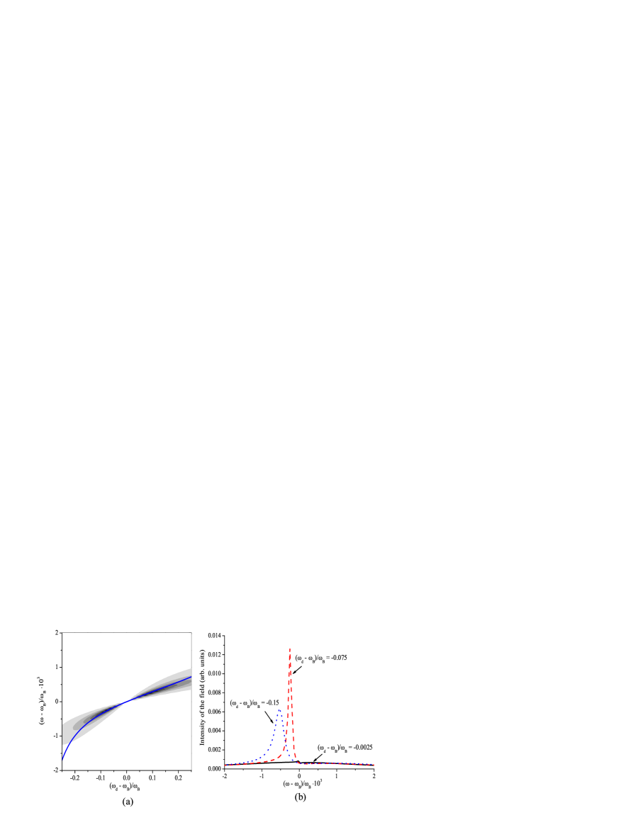
Figure 10: (color online)(a). The luminescence spectrum of the Bragg $40$ layers structure with the defect layer inserted at the middle of the structure. The intensity of the emitted field is plotted as a function of frequency (the vertical axis) for structures with the defect layer characterized by different $\omega_{d}$ (the horizontal axis). The solid line depicts the position of the maximum of the transmission as obtained in Eq. (61). The parameters of the structure are the same as in Fig. 4a. (b). Explicit form of the luminescence spectrum of the defect structure for several values of the defect resonant frequency $\omega_{d}$.

As follows from this consideration, the defect layer inserted into a MQW structure leads to the appearance of a transparency resonance with the width $\sim\gamma$. The position of the maximum of the emission is determined by the interplay between the maximum of the transmission and the decay of the exciton luminescence at frequencies away from $\omega_{0}$. The maximum of the field intensity, therefore, is expected at frequencies shifted from $\omega_{min}$ towards $\omega_{0}$.

In Figure 10 we plot the luminescence spectrum for the structures with different width of the defect layer. The spectrum is obtained by performing direct summation in Eq. (48) using the invariant embedding methodDeych et al. (1999) for finding the partial transfer matrices. As one can see, the numerical calculations confirm the simple analysis provided above and demonstrate a sharp rise in the luminescence due to the defect state.

IV.4 Absorption and luminescence spectra

According to the Kirchhoff’s law all emitting system in thermodynamic equilibrium must demonstrate an universal relationship between their absorption and emission spectra. Such a relationship exists even in non-equilibrium but stationary situations such as luminescence in the regime of steady state excitation. To establish such a relationship for a particular system, however, is not always a straightforward task. For instance, authors of Ref. Stanley et al., 1996 managed to establish such a relationship for quantum well excitons only as an approximation. At the same time, this relationship might be rather important because it could allow to relate to each other various microscopic characteristics of a system under consideration independently of particular microscopic model used for their calculation. Here we will use the approach to description of resonant photonic crystals developed in the present paper as well as in Refs. Erementchouk et al., 2005, 2006 in order to derive an exact relation between absorption and emission spectra of resonant photonic crystals.

A traditional definition of absorbance, $A(\omega)$, of an open one-dimensional dielectric structure has the form

$$A(\omega)=1-T(\omega)-R(\omega)$$ (62)

where the last two terms represent transmission and reflection coefficients respectively. This form can be effectively used to carry out a thermodynamical derivation of the relation between emission and absorption specifically tailored for one-dimensional systems. Let’s assume that our one-dimensional structure is bounded by vacuum on its left-hand side and by a homogeneous dielectric medium with refractive index $n_{b}$ on its right-hand side. The derivation is based on the statement that in equilibrium total photon flux out of the system must be equal to zero. This total flux includes the flux of emitted photons, $\Phi_{em}$, and the flux of the incident and transmitted/reflected photons, $\Phi_{i}$, $\Phi_{t}$, and $\Phi_{r}$, respectively. $\Phi_{em}$ can be calculated as

$$\Phi_{em}=I_{0}(\omega)d\omega\frac{dq_{x}dq_{y}}{(2\pi)^{3}},$$ (63)

where $I_{0}$ is the equilibrium luminescence intensity, and $q_{x,y}$ represent conserving in-plane components of the photons’ wave vector. The incoming and reflected fluxes in vacuum can be presented as

$$\begin{split}\Phi_{i}+\Phi_{r}=\hbar\omega cN_{ph}^{0}(\omega)\left[1-R(\omega)\right]\frac{dq_{x}dq_{y}dq_{z}}{(2\pi)^{3}}\\ =\hbar\omega N_{ph}^{0}(\omega)\left[1-R(\omega)\right]d\omega\frac{dq_{y}dq_{z}}{(2\pi)^{3}}\>,\end{split}$$ (64)

where $N_{ph}^{0}(\omega)$ is the equilibrium photon occupation number. The last contribution to the flux of photons in vacuum comes from the photons transmitted from the medium on the right-hand side of the structure. This flux can be written down as

$$\Phi_{t}=\frac{c}{n_{b}}N_{ph}^{0}(\omega)\tilde{T}(\omega)\frac{dq_{x}dq_{y}dq_{z}}{(2\pi)^{3}}\\ =\hbar\omega N_{ph}^{0}(\omega)\tilde{T}(\omega)d\omega\frac{dq_{y}dq_{z}}{(2\pi)^{3}}$$ (65)

where $\tilde{T}$ stands for the transmission coefficient of light incident on the system from the right-hand side, and we took into account the refractive index $n_{b}$ of the medium on the right. Combining Eq.(63) with Eq.(64),(65) and with the requirement of the zero total flux we can write down

$$\hbar\omega N_{ph}^{0}(\omega)\left[1-R(\omega)-\tilde{T}(\omega)\right]=I_{0}(\omega)$$ (66)

Taking into account Eq.(62) and the fact that due to the time reversal symmetry transmission coefficients, $\tilde{T}$ for the wave incident from right is equal to the one describing waves incident from left we obtain a final form of the Kirchhoff’s law for one-dimensional layered structures

$$I_{0}(\omega)=\hbar\omega N_{ph}^{0}(\omega)A(\omega)$$ (67)

Equilibrium photon distribution function at low temperatures $k_{B}T\ll\hbar\omega$ can be approximated by $\exp{(-\hbar\omega/k_{B}T)}$.

The derivation of Eq. (67) is based on two main assumptions: zero photon flux, and time reversal symmetry, both of which are valid for any kind of steady state, not necessarily equilibrium, situations. In non-equilibrium cases, however, the concept of photon distribution function, $N_{ph}(\omega)$, appearing in Eq.(67), becomes ambiguous, and generalization of this equation to these situations is not straightforward. Nevertheless, under certain circumstances, a relation similar to Eq.(67) can be obtained for such non-equilibrium phenomena as luminescence under steady state excitation. Results of numerous studies of exciton photo-luminescence in QW (see, for instance, Ref.Ivchenko, 2005; Damen et al., 1990) indicate that in the case of non-resonant photo-excitation of luminescence at the moderately low temperatures where the main contribution to luminescence already comes from free excitons, the following kinetic of luminescence can be assumed. Originally excited electron-hole pairs first relax through phonon-assisted processes to high energy states with in-plane wave numbers $k$ corresponding to non-radiative ”dark” excitonsDamen et al. (1990). These states live long enough to come in quasi-equilibrium with the crystal lattice, so that they can be characterized by a Boltzmann distribution $f_{B}(E)\propto\exp{[-(E-\mu)/k_{B}T]}$. The dark exciton act as a source of exciton luminescence, and, according to calculations presented in Appendix, the photoluminescence intensity $I(\omega)$ is a linear functional of the exciton distribution function, $f_{B}(E)$. Term $\exp{(\mu/k_{B}T)}$ in the Boltzmann distribution can be factored out, and the remaining expression reproduces equilibrium emission intensity. Thus for the intensity of the luminescence we can write $I(\omega)=\exp{(\mu/k_{B}T)}I_{0}(\omega)$, from which it follows that $I(\omega)$ and $A(\omega)$ are related to each other as

$$I(\omega)=\hbar\omega\exp{(\mu/k_{B}T)}N_{ph}^{0}(\omega)A(\omega)$$ (68)

Experimental verification of the relation given by Eq.(68) can provide useful qualitative information about the distribution of excitons and their kinetics either this relation is confirmed or not. Eq.(68) can be applied to emission and absorption of each QW constituting the structure, and if the distribution functions of excitons are identical in each well, to the entire MQW structure as well.

The established relation between emission and absorption is based on thermodynamical arguments and depends little on the details of the structures under consideration. It appears useful to compare this relation with the one derived on the basis of solution of Maxwell equations for the particular model of MQW structure considered in this paper. To this end it is more convenient to use an alternative expression for absorption, which follows directly from the definition of Poynting vector and energy conservation:

$$A=-\frac{\oint\mathbf{S}\cdot d\mathbf{a}}{S_{0}L_{x}L_{y}}$$ (69)

where $\mathbf{S}$ is the Poynting vectors of outgoing radiation respectively, $S_{0}$ and $L_{x}$, $L_{y}$ are the magnitude of the Poynting vector of the incoming radiation and the transverse dimensions of the sample respectively; the integral is taken over a surface enclosing the entire sample. The particular convenience of Eq. (69) for 1D structures stems from the fact that this expression allows for expressing the absorption in terms of the fields at the boundaries of the structure. Assuming that the incoming radiation impinges on the structure from the left, where the space is filled with the medium with refractive index $n_{L}$, one can obtain for the absorption coefficient

$$A=\left.\frac{1}{2ik_{L}\mid E_{0}\mid^{2}}\left(E\frac{dE^{*}}{dz}-E^{*}\frac{dE}{dz}\right)\right|_{z_{L}}^{z_{R}},$$ (70)

where $k_{L}$ is the wave number of the field in the surrounding medium to the left of the sample, and $E_{0}$ is the electric field amplitude of the incoming radiation. Multiplying Eq. (7) without sources and its conjugate by $E^{*}$ and $E$, respectively, and integrating over the entire structure one obtains

$$A=\frac{4\pi\omega^{2}}{k_{L}c^{2}}\sum_{m}\left|\int_{QW}dz\,\Phi_{m}(z)E(z)\right|^{2}\mathrm{Im}\,\chi_{m}.$$ (71)

This expression has clear physical meaning. It shows that the absorption of the resonant photonic crystal is the sum of independent contributions of all quantum wells. Each contribution has an expected form of the product of the imaginary part of the exciton susceptibility and a term proportional to the projection of the em field onto the exciton state in the well. In order to find a relation between the absorption and the emission spectra we calculate the absorption of the wave of unit intensity incident normally from the left. Electric field inside each well, and respective integrals in Eq.(71), can be found using standard transfer-matrix technique (see, for instance Ref. Ivchenko et al., 2004; Erementchouk et al., 2005). As a result Eq. (71) can be presented in the form explicitly containing the same Green’s functions as one used in this paper, Eq.(41):

$$A=\frac{c}{n_{L}\pi\omega}\sum_{m}\frac{\mathrm{Im}\,\chi_{m}}{|\chi_{m}|^{2}}\left|\frac{4\pi\omega^{2}}{c^{2}}\tilde{\chi}_{m}\right|^{2}\left|\mathcal{G}^{(s)}(m){\varphi_{m}}_{1}+\mathcal{G}^{(a)}(m){\varphi_{m}}_{2}\right|^{2}.$$ (72)

Comparing this expression with Eq. (40) (with terms proportional to $F_{1}$ and $F_{2}$ omitted) we can relate the emitted intensity to the absorption coefficient for a single $m$-th well of the structure

$$\mathcal{I}_{-}(m)=\frac{\pi n_{L}\omega}{c}\frac{\Xi_{m}|\chi_{m}|^{2}}{\mathrm{Im}\,\chi_{m}}A(m)=\frac{\pi n_{L}\omega}{c}\frac{\Xi_{m}\alpha}{\gamma}A_{(}m)$$ (73)

where, in the second expression, we assumed that exciton susceptibility has a Lorentzian form and is described by Eq. (18). This assumption can be violated under several circumstances, for instance, when several exciton levels spectrally overlap and contribute to the emission,Erementchouk (2005) or in the presence of the inhomogeneous broadening of excitons. If the latter case is treated in the effective medium approximation, as was discussed previously in this paper and in Refs. Deych et al., 2004; Andreani et al., 1998, it results in an effective susceptibility with non-Lorentzian shape.

In order to derive a global relation between emission and absorption for the entire structure, Eq. (73) has to be summed over all wells. If all wells are identical, i. e. the source functions and non-radiative decay rates in all wells are the same, the summation is trivial and the global relation between absorption and emission coefficients has again the form of Eq. (73). Comparing this result with Eq.(68) we can establish relationship between microscopic parameters such as the strength of the exciton-light coupling, characterized by $\alpha$, non-radiative decay rate $\gamma$, the source function $\Xi$, which is proportional to polarization correlation function, and photon distribution function, $N_{ph}^{(0)}$:

$$\hbar N_{ph}^{(0)}(\omega)=\frac{\pi}{c}\exp{(-\mu/k_{B}T)}\frac{\Xi(\omega)\alpha}{\gamma(\omega)}$$ (74)

Since the photon distribution function is practically independent of frequency on the scale of frequencies considered in this paper, Eq.(74) is consistent with an assumption that both $\gamma$ and $\Xi_{m}$ are frequency independent quantities. Taking into account also that $1/\omega$ term in Eq.(73) also changes very weakly on the same scale, we can conclude on the basis of both Eq.(67) and Eq.(73) that emission and absorption spectra in our case are directly proportional to each other: $\mathcal{I}_{-}(\omega)\propto A(\omega)$. Numerical evaluation of the respective expressions completely confirm this conclusion.

The assumption of all wells being the same, however, may violate in photoluminescent experiments due to attenuation of the pumping radiation. As a result, different wells may be characterized by different exciton distribution functions, and consequently by different source functions. In this case, while Eq.(73) remains valid locally for any particular well, its global version is not true anymore. This results in loss of the direct proportionality between absorption and emission spectra of our structures. This is clearly seen from Fig.7, which shows modification of emission intensity caused by attenuation of pump, while absorption spectra obviously are not affected by this circumstance.

V Conclusion

In the present paper we studied spectrum of non-coherent radiation emitted by one-dimensional resonant photonic crystal structures. While for concreteness we focused on exciton luminescence in multiple-quantum-well structures, the general theoretical framework developed in this work can be applied to other structures of this sort. The results obtained in the paper can be classified in two groups. First, we have developed a powerful method of solving general linear response type of problems for one-dimensional layered structures of general type. The problem of luminescence of one-dimensional resonant photonic structures is just one example of such problems, in which one is looking for the radiative response of the system caused by incoherent periodically distributed emitters. Our approach allows expressing Greens’ function of the structure in terms of transfer matrices describing propagation of the radiation through the system. As a result we are able to present the spectrum of the emitted light in terms of reflection and transmission coefficients of the structure in question. Also, with the help of a special version of transfer-matrix description of transmission/reflection properties of resonant photonic crystals developed in recent Refs. Erementchouk et al., 2006 and Erementchouk et al., 2005 we were able to obtain a closed analytical expression for the spectrum of luminescence of an resonance photonic crystal structure with an arbitrary number of identical periods. An important characteristics of these general results is that they are obtained in terms of particular solutions of an initial value problem for a structure with an arbitrary spatial profile of the refractive index. The latter problem can always be easily solved either analytically, or in most cases at least numerically, and, therefore, emission characteristics are expressed in our approach in terms of easily accessible quantities.

The second group of the results is concerned with application of our general formalism to the particular case of Bragg or near-Bragg multiple-quantum-well structures. We analyzed the luminescence spectrum of these structures and established its main qualitative and quantitative characteristics. In particular, we explained the absence of luminescence in the spectral region of polariton stop-band, which was shown to be due to a combination of two factors: diminishing of transmission of light through the structure in the vicinity of the exciton frequency, and a significant spectral separation of the latter from transparent regions because of formation of the wide band-gap. It is interesting to note that this result agrees with quantum-field calculations of Ref.Schäfer et al., 2006, where similar effect was called ”subradiance”. Our calculations show, however, that this effect can be explained on purely classical ground.

We also considered modification of the spectrum when the period of the structure becomes slightly de-tuned from the exact Bragg conditions. Comparison of our calculations with experimental spectra demonstrated an important role played by inhomogeneous broadening of excitons in formation of the spectra of luminescence of the structures under consideration. We also showed that these spectra are influenced by a great deal of other effects such as attenuation of the pump, or presence of cladding layers in the structure. We found that our calculations produce good agreement with experiment in terms of positions of the peaks of the luminescence, but not for the relative height of the peaks. This, however, is not very surprising, because the intensities of the peaks depend on many various circumstances. One of the most intriguing effect, which was not considered in the paper, but which could significantly influence the distribution of the luminescence intensity between its peaks, is acoustic phonon-induced scattering between collective exciton polariton states formed in quasi-Bragg MQW structures. This possibility is supported by the fact that spectral separation between luminescence peaks in typical experimentsHubner et al. (1999); Mintsev et al. (2002) is of the same order of magnitude ($1meV$) as an average energy of acoustic phonons in $GaAs$. Consideration of this effect is out of the scope of the current paper, but will be presented in the subsequent publications.

In order to achieve a better understanding of luminescence of the quasi-Bragg structures, one needs additional experimental data, which would provide information for assessing the role of different effects. For instance, since one can, to some extent, control inhomogeneous broadening of excitons by growth conditions, luminescence measurements on a series on sample grown under different conditions could clarify the role of inhomogeneous broadening. Another possibility can be to excite luminescence by pumping the sample from both sides, which will reduce effects due to inhomogeneity of source function, and assess the role of this effect. Temperature dependence of the intensity of the luminescent maxima can be used to verify the role of acoustic phonon scattering.

An interested question studied in the last section of the paper is concerned with relation between luminescence and absorption spectra in multiple-quantum-well structures. First, using thermodynamical arguments we derived a version of Kirchhoff’s law specifically adapted for one-dimensional structures under consideration. Then, using developed formalism, we were able to establish the relation between luminescence and absorption in terms of microscopic characteristics of the system such as polarization correlation function and exciton susceptibility. Comparing the two results we established a relation between the microscopic parameters consistent with the Kirchhoff’s law. In particular, we found that if the spectral region of interest is small compared to the characteristic energy scale of the photon distribution function, both polarization correlation function and the non-radiative decay rate of excitons can be considered as frequency independent.

Appendix

In this Appendix we will provide a sketch of quantum-mechanical calculations of luminescence from a single quantum well. The objective of this exercise is to provide a microscopic justification for the quasi-classical approach employed in the paper, and demonstrate relations between phenomenological source function $\Sigma(\rho,t)$ and microscopical characteristics of the system. This relation can be derived only by using the second quantization of the exciton and photon states and a relevant microscopic kinetic equation. Here we will demonstrate the second-quantization approach for a single QW-structure with a QW layer sandwiched between semi-infinite barriers. For simplicity, the dielectric contrast $n_{w}-n_{b}$ is set to zero.

The 2D ${\bm{k}}$-space is naturally divided into two regions, radiative and nonradiative, respectively, with $k<k_{0}\equiv(\omega_{0}/c)n_{b}$ and $k>k_{0}$. In the process of relaxation of electron-hole pairs non-radiative excitons with $k>k_{0}$ are being populated firstDamen et al. (1990), and we assume that, for these excitons the criterion $\bar{k}l\gg 1$ for validity of the Boltzmann kinetic equation is fulfilled. Here ${\bar{k}}^{2}$ is the average value of $k^{2}$ describing the spread of exciton population in the ${\bm{k}}$-space, $l$ is the 2D exciton mean free-path length, $l=(\hbar\bar{k}/M)\tau_{p}$, $\tau_{p}$ is the exciton momentum scattering time, and $M$ is the exciton in-plane effective mass. For 3D photons we introduce a quantization box of the volume $V=SL$ with the macroscopic interface area $S$ and the macroscopic length $L$ along the QW growth direction.

In order to calculate the spectral intensity of light emitted by excitons in the QW we apply the Keldysh diagram techniqueLifshits and Pitaevsky (1981); Keldysh (1964), in a way similar to one used for the description of exciton or exciton-polariton photoluminescence in bulk crystals, see for instance, Ref.  Ivchenko et al., 1977, 1989. In this method the intensity $I_{\bm{q}}$ can be written as

$$I_{\bm{q}}=\hbar\omega_{\bm{q}}w_{\bm{q}}\>,\>w_{\bm{q}}=-\lim_{\gamma\to+0}\left(\frac{\gamma}{\pi}\int D^{-+}_{{\bm{q}},\omega}~{}d\omega\right)\>.$$ (75)

Here $w_{\bm{q}}$ is the emission rate of a photon with the 3D photon wave vector ${\bm{q}}$, $D^{-+}_{{\bm{q}},\omega}$ is the photon Green function presented in the left-hand side of the diagram equation shown in Fig. 11 by an short-dashed line connecting the lower and higher horizontal parts of the Keldysh contour labeled ”+” and ”-”, respectively; $\gamma$ is a positive photon damping rate which is introduced for the formal reasons in order to stabilize the photon distribution in the steady-state regime [$(2\gamma)^{-1}$ is the photon lifetime in the quantization box]. In the end $\gamma$ is set to $+0$ since in a single QW structure with the microscopic length $L$ the actual photon damping rate is negligible. Equation (75) is derived taking into account that, in the steady-state regime, one has

$$D^{-+}_{{\bm{q}},\omega}=-2\pi N_{\bm{q}}\left(\frac{1}{\pi}\frac{\gamma}{(\omega-\omega_{\bm{q}})^{2}+\gamma^{2}}\right)\>,$$ (76)

where $\omega_{\bm{q}}=cq/n_{b}$, $N_{\bm{q}}=w_{\bm{q}}/(2\gamma)$ is the steady-state photon distribution function. Here the temperature is assumed to be very small as compared to the exciton excitation energy, which allows one to neglect the equilibrium photon-state population. Note that the close-to-normal energy flux in the frequency range $d\omega$ and within the area $d^{2}q_{\parallel}$ in the plane $(q_{x},q_{y})$ is related with $I_{\bm{q}}$ by

$$dI(\omega)=\frac{d^{2}q_{\parallel}d\omega}{(2\pi)^{3}}\frac{Ln_{b}}{c}I_{\bm{q}}\>.$$

The Green function $D^{-+}_{{\bm{q}},\omega}$ is found from the diagram equation presented in Fig. 11. The diagrams on the right-hand side of the equation describe the acoustic-phonon assisted scattering of an exciton from the non-radiant state ${\bm{k}}^{\prime}$ to the radiative state ${\bm{q}}_{\parallel}$, where ${\bm{q}}_{\parallel}$ is the in-plane component of ${\bm{q}}$; ${\bm{Q}}$ and $\omega_{\bm{Q}}$ are the phonon wave vector and frequency. In Fig. 11 the short-dashed lines mean ${\rm i}D^{s^{\prime}s}_{{\bm{q}}\omega}$, where the superscripts $s^{\prime},s=\pm$ show the position of the ends of the photon Green functions,

$$D^{--}_{{\bm{q}}\omega}=-\left(D^{++}_{{\bm{q}}\omega}\right)^{*}=\frac{1}{\omega-\omega_{\bm{q}}+{\rm i}\gamma}\>.$$

The solid lines represent exciton Green functions ${\rm i}G^{s^{\prime}s}_{{\bm{k}}\omega}$, given by

$$G^{-+}_{{\bm{k}}^{\prime},\omega\pm\Omega_{\bm{Q}}}=-2\pi f_{{\bm{k}}^{\prime}}\left(\frac{1}{\pi}\frac{\Gamma_{{\bm{k}}^{\prime}}}{(\omega\pm\Omega_{\bm{Q}}-\omega^{({\rm exc})}_{{\bm{k}}^{\prime}})^{2}+\Gamma_{{\bm{k}}^{\prime}}^{2}}\right)\>,$$

$$G^{--}_{{\bm{k}}\omega}=-\left(G^{++}_{{\bm{k}}\omega}\right)^{*}=\frac{1}{\omega-\omega^{({\rm exc})}_{\bm{k}}+{\rm i}(\Gamma_{\bm{k}}+\Gamma_{0{\bm{k}}})}\>,$$

$\omega^{({\rm exc})}_{\bm{k}},\Gamma_{\bm{k}}$ and $\Gamma_{0{\bm{k}}}$ are the exciton excitation energy, non-radiative and radiative damping rates, $f_{{\bm{k}}^{\prime}}$ is the exciton distribution function assumed to be small, $f_{{\bm{k}}^{\prime}}\ll 1$. Each vortex represents the matrix element of exciton-phonon ($V_{\bm{Q}}$) or exciton-photon ($M_{{\bm{q}}_{\parallel}}$) interaction multiplied by $\pm{\rm i}/\hbar$, plus for the lower part and minus for the upper part of the Keldysh contour. Since we neglect the damping of acoustic phonons

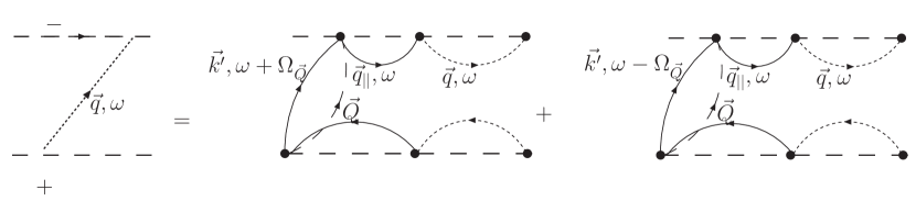
Figure 11: .

the upward and downward phonon (long-dashed) lines can simply be replaced by the factors $m_{\bm{Q}}$ and $m_{\bm{Q}}+1$, where $m_{\bm{Q}}$ is the phonon occupation number. For a process described by any vortex the conservation of the in-plane wave vectors should be satisfied. In particular, ${\bm{k}}^{\prime}={\bm{k}}\pm{\bm{Q}}_{\parallel}$ for the phonon emission and absorption, respectively. As a result, we obtain

$${\rm i}D^{-+}_{{\bm{q}},\omega}=\frac{1}{\hbar^{4}}\sum_{{\bm{k}}^{\prime},{\bm{Q}}}|D^{--}_{{\bm{q}}\omega}|^{2}|G^{--}_{{\bm{q}}_{\parallel}\omega}|^{2}|M_{{\bm{q}}_{\parallel}}|^{2}|V_{\bm{Q}}|^{2}$$

$$\times{\rm i}[G^{-+}_{{\bm{k}}^{\prime},\omega-\Omega_{\bm{Q}}}m_{\bm{Q}}\ \delta_{{\bm{k}}^{\prime},{\bm{k}}-{\bm{Q}}_{\parallel}}+G^{-+}_{{\bm{k}}^{\prime},\omega+\Omega_{\bm{Q}}}(m_{\bm{Q}}+1)\ \delta_{{\bm{k}}^{\prime},{\bm{k}}+{\bm{Q}}_{\parallel}}]\>.$$

where summation over $k\prime$ is carried only over non-radiative states because the population of the radiative states is assumed to be negligible. It follows then that the photon generation rate $w_{\bm{q}}$ in Eq. (75) can be presented in the form

$$w_{\bm{q}}=\frac{W^{({\rm phot})}(\omega_{\bm{q}},{\bm{q}}_{\parallel})\ W^{({\rm phon})}(\omega_{\bm{q}},{\bm{q}}_{\parallel})}{2(\Gamma_{{\bm{q}}_{\parallel}}+\Gamma_{0{\bm{q}}_{\parallel}})}\>,$$ (77)

$$W^{({\rm phot})}(\omega,{\bm{k}})=\frac{2\pi}{\hbar^{2}}|M_{{\bm{k}}}|^{2}\ \frac{1}{\pi}\frac{\Gamma_{{\bm{k}}}+\Gamma_{0{\bm{k}}}}{(\omega-\omega^{({\rm exc})}_{{\bm{k}}})^{2}+(\Gamma_{{\bm{k}}}+\Gamma_{0{\bm{k}}})^{2}}\>,$$

$$W^{({\rm phon})}(\omega,{\bm{k}})=\frac{2\pi}{\hbar^{2}}\sum_{{\bm{k}}^{\prime},{\bm{Q}}}|V_{\bm{Q}}|^{2}f_{{\bm{k}}^{\prime}}[m_{\bm{Q}}\ \delta(\omega-\Omega_{\bm{Q}}-\omega^{({\rm exc})}_{{\bm{k}}^{\prime}})\ \delta_{{\bm{k}}^{\prime},{\bm{k}}-{\bm{Q}}_{\parallel}}$$

$$+\ (m_{\bm{Q}}+1)\ \delta(\omega+\Omega_{\bm{Q}}-\omega^{({\rm exc})}_{{\bm{k}}^{\prime}})\ \delta_{{\bm{k}}^{\prime},{\bm{k}}+{\bm{Q}}_{\parallel}}]\>.$$

Here, taking into account the condition $\bar{k}l\gg 1$ we replaced in the last equation the phonon’s resonance Lorentzians by Dirac delta-functions.

In the Bragg and quasi-Bragg structures, the radiative excitonic states $|n,{\bm{k}}\rangle$ in different wells $n$ with the same wave vector ${\bm{k}}$ are strongly coupled by the electromagnetic field. In contrast, excitons with ${\bm{k}}$ satisfying the conditions $k>k_{0}$, $\sqrt{k^{2}-k_{0}^{2}}d\gg 1$ are decoupled and can be considered as excitations isolated in particular wells. The photon emission outgoing from a given QW can be described by Eq. (77) as well or, equivalently. On the other hand, the propagation of this outgoing light wave through the whole MQW structure accompanied by its reabsorption and escape into the vacuum or substrate, can be described classically.

Instead of the above microscopical consideration, in the main part of the paper the photoluminescence spectra are calculated with the help of a quasi-classical Langevin-like approach by introducing the random source $\Sigma_{m}({\bm{\rho}},\omega)$ into expression for exciton polarization, see Eq. (2). Now, the explicit expression for the correlator $\Xi_{m}(\omega,{\bm{k}})$ of the random sources in Eq. (46) can be readily found from Eq. (77). In particular, one has

$$\Xi_{m}(\omega,0)=\frac{2\pi q}{\hbar\varepsilon_{b}\Gamma_{0}^{2}}|M_{0}|^{2}W^{(\rm phon)}(\omega,0)\left[\int\Phi_{m}(z)dz\right]^{2}\>,$$ (78)

where $\Gamma_{0}$ is the radiative damping rate of an exciton with ${\bm{k}}=0$ excited in a single QW structure.

The applicability of the Langevin method can be justified by considering Heisenberg equations of motion for exciton annihilation ($\hat{c}_{\bm{k}}$) and creation ($\hat{c}^{\dagger}_{\bm{k}}$) operators. For the exciton-phonon Hamiltonian

$$\sum_{{\bm{k}}{\bm{k}}^{\prime}{\bm{Q}}}\hat{c}^{\dagger}_{\bm{k}}\hat{c}_{{\bm{k}}^{\prime}}\left(\hat{d}_{\bm{Q}}V_{\bm{Q}}\delta_{{\bm{k}}^{\prime},{\bm{k}}-{\bm{Q}}_{\parallel}}+\hat{d}^{\dagger}_{\bm{Q}}V_{\bm{Q}}^{*}\delta_{{\bm{k}}^{\prime},{\bm{k}}+{\bm{Q}}_{\parallel}}\right)\>,$$

where $\hat{d}_{\bm{Q}},\hat{d}^{\dagger}_{\bm{Q}}$ are the acoustic-phonon annihilation and creation operators, one obtains

$$\dot{\hat{c}}_{\bm{k}}(t)=-\omega^{({\rm exc})}_{\bm{k}}\hat{c}_{\bm{k}}(t)-\frac{\rm i}{\hbar}M_{\bm{k}}^{*}\hat{b}_{\bm{k}}(t)+\hat{\xi}_{\bm{k}}(t)$$ (79)

with $\hat{b}_{\bm{k}}$ being the photon annihilation operator. Here term

$$\hat{\xi}_{\bm{k}}(t)=-\frac{\rm i}{\hbar}\sum_{{\bm{k}}^{\prime}{\bm{Q}}}\left(V_{\bm{Q}}\hat{d}_{\bm{Q}}\delta_{{\bm{k}}^{\prime},{\bm{k}}-{\bm{Q}}_{\parallel}}+V_{\bm{Q}}^{*}\hat{d}^{\dagger}_{\bm{Q}}\delta_{{\bm{k}}^{\prime},{\bm{k}}+{\bm{Q}}_{\parallel}}\right)\hat{c}_{{\bm{k}}^{\prime}}$$

playes the role of the Langevin source operator, and summation again is carried over only values of $k\prime$ corresponding to non-radiative states. Fourier transform of the correlator of this operator

$${\rm i}\int d\tau\ \langle\hat{\xi}^{\dagger}_{\bm{k}}(t)\hat{\xi}_{\bm{k}}(t+\tau)\rangle{\rm e}^{{\rm i}\omega\tau}$$

is equal to $W^{({\rm phon})}(\omega,{\bm{k}})$, which agrees with Eq. (78) if we take into account the relation between the 2D exciton envelope function and exciton-induced polarization $P_{\rm exc}$.

References

- Yablonovitch (1987) E. Yablonovitch, Phys. Rev. Lett. 58, 2059 (1987).
- (2) J. D. Joannopoulos, R. D. Meade, and J. N. Winn, Photonic crystals: Molding the flow of light (Princeton University Press, Princeton, USA, ????).
- Woldeyohannes and John (2003) M. Woldeyohannes and S. John, J. Opt. B: Quantum Semiclass. Opt. 5, R43 (2003).
- Megens et al. (1999) M. Megens, J. E. G. J. Wijnhoven, A. Lagendijk, and W. L. Vos, Phys. Rev. A 59, 4727 (1999).
- Li and Zhang (2001) Z.-Y. Li and Z.-Q. Zhang, Phys. Rev. B 63, 125106 (2001).
- Florescu and John (2001) M. Florescu and S. John, Phys. Rev. A 64, 033801 (2001).
- Vats et al. (2002) N. Vats, S. John, and K. Busch, Phys. Rev. A 65, 043808 (2002).
- Barth et al. (2006) M. Barth, R. Schuster, A. Gruber, and F. Cichos, Phys. Rev. Lett. 96, 243902 (2006).
- Brueck et al. (2003) S. R. Brueck, V. A. Smagley, and P. G. Eliseev, Phys. Rev. E 68, 036608 (2003).
- Hoekstra and Elrofai (2005) H. J. W. M. Hoekstra and H. B. H. Elrofai, Phys. Rev. E 71, 046609 (2005).
- Savona et al. (1996) V. Savona, F. Tassone, C. Piermarocchi, A. Quattropani, and P. Schwendimann, Phys. Rev. B 53, 13051 (1996).
- Hayes et al. (1998) G. Hayes, S. Haacke, M. Kauer, R. Stanley, R. Houdre, U. Oesterle, and B. Deveaud, Phys. Rev. B 58, R10175 (1998).
- Kuzmiak and Maradudin (1997) V. Kuzmiak and A. Maradudin, Phys. Rev. B 55, 7427 (1997).
- Deych et al. (1998) L. Deych, D. Livdan, and A. Lisyansky, Phys. Rev. E 57, 7254 (1998).
- Nojima (2000) S. Nojima, Phys. Rev. B 61, 9940 (2000).
- Sivachenko et al. (2001) A. Y. Sivachenko, M. E. Raikh, and Z. V. Vardeny, Phys. Rev. A 64, 013809 (2001).
- Christ et al. (2003) A. Christ, S. Tikhodeev, N. Gippius, J. Kuhl, and G. H., Phys. Rev. Lett. 91, 183901 (2003).
- Huang et al. (2003) K. Huang, P. Bienstman, J. Joannopoulos, K. Nelson, and S. Fan, Phys. Rev. Lett. 90, 196402 (2003).
- Toader and John (2004) O. Toader and S. John, Phys. Rev. E 70, 046605 (2004).
- Pilozzi et al. (2004) L. Pilozzi, A. D’Andrea, and K. Cho, Phys. Rev. B 69, 205311 (2004).
- Ivchenko and Poddubny (2006) E. Ivchenko and A. Poddubny, Fiz. Tverd. Tela (S.-Peterburg) 48, 540 (2006), [Phys. Solid. State 48, 561 (2006)].
- Ivchenko et al. (2004) E. L. Ivchenko, M. M. Voronov, M. V. Erementchouk, L. I. Deych, and A. A. Lisyansky, Phys. Rev. B 70, 195106 (2004).
- Ivchenko et al. (1994) E. L. Ivchenko, A. I. Nesvizhskii, and S. Jorda, Phys. Solid State 36, 1156 (1994).
- Erementchouk et al. (2006) M. V. Erementchouk, L. I. Deych, and A. A. Lisyansky, Phys. Rev. B 73, 115321 (2006).
- Schäfer et al. (2006) M. Schäfer, M. Werchner, W. Hoyer, M. Kira, and S. W. Koch, Phys. Rev. B 74, 155315 (2006).
- Kira et al. (1999) M. Kira, F. Jahnke, W. Hoyer, and S. Koch, Prog. Quant. Electr. 23, 189 (1999).
- Ivchenko (2005) E. L. Ivchenko, Optical Spectroscopy of Semiconductor Nanostructures (Alpha Science International Ltd., Harrow, U.K., 2005).
- Ivchenko (1991) E. L. Ivchenko, Sov. Phys. Solid State 33, 1344 (1991).
- Hubner et al. (1999) M. Hubner, J. Prineas, C. Ell, P. Brick, E. Lee, G. Khitrova, H. Gibbs, and S. Koch, Phys. Rev. Lett. 83, 2841 (1999).
- Deych et al. (2004) L. I. Deych, M. V. Erementchouk, and A. A. Lisyansky, Phys. Rev. B 69, 75308 (2004).
- Morse and Feshbach (1953) P. M. Morse and H. Feshbach, Methods of theoretical physics, vol. 1 (McGraw-Hill, Tokyo, 1953).
- Morawitz (1969) H. Morawitz, Phys. Rev. 187, 1792 (1969).
- Dowling and Bowden (1992) J. P. Dowling and C. M. Bowden, Phys. Rev. A 46, 612 (1992).
- Stanley et al. (1996) R. P. Stanley, R. Houdré, C. Weisbuch, U. Oesterle, and M. Ilegems, Phys. Rev. B 53, 10995 (1996).
- Dodd (1997) J. N. Dodd, Physica Scripta 1997, 88 (1997).
- Xu et al. (2000) Y. Xu, R. K. Lee, and A. Yariv, Phys. Rev. A 61, 033807 (2000).
- Erementchouk et al. (2005) M. V. Erementchouk, L. I. Deych, and A. A. Lisyansky, Phys. Rev. B 71, 235335 (2005).
- Deych and Lisyansky (2000) L. I. Deych and A. A. Lisyansky, Phys. Rev. B 62, 4242 (2000).
- Mintsev et al. (2002) A. Mintsev, L. Butov, C. Ell, S. Mosor, G. Khitrova, and H. Gibbs, JETP Lett. 76, 637 (2002).
- Andreani et al. (1998) L. C. Andreani, G. Panzarini, A. V. Kavokin, and M. R. Vladimirova, Phys. Rev. B 57, 4670 (1998).
- Stanley et al. (1993) R. P. Stanley, R. Houdré, U. Oesterle, M. Ilegems, and C. Weisbuch, Phys. Rev. A 48, 2246 (1993).
- Liu (1997) N. Liu, Phys. Rev. B 55, 4097 (1997).
- Figotin and Gorentsveig (1998) A. Figotin and V. Gorentsveig, Phys. Rev. B 58, 180 (1998).
- Ozaki et al. (2004) R. Ozaki, Y. Matsuhisa, M. Ozaki, and K. Yoshino, Appl. Phys. Lett. 84, 1844 (2004).
- Deych et al. (1987) L. Deych, A. Yamilov, and A. Lisyansky, Phys. Rev. B 64, 075321 (1987).
- Citrin (1995) D. S. Citrin, Appl. Phys. Lett. 66, 994 (1995).
- Deych and Lisyansky (1998) L. I. Deych and A. A. Lisyansky, Phys. Lett. A 243, 156 (1998).
- Deych et al. (2000) L. Deych, A. Yamilov, and A. Lisyansky, Optics letters 25, 1705 (2000).
- Deych et al. (2003) L. I. Deych, M. V. Erementchouk, and A. A. Lisyansky, Appl. Phys. Lett. 83, 4562 (2003).
- Deych et al. (1999) L. Deych, A. Yamilov, and A. Lisyansky, Phys. Rev. B 59, 11339 (1999).
- Damen et al. (1990) T. C. Damen, J. Shah, D. Y. Oberli, D. S. Chemla, J. E. Cunningham, and J. M. Kuo, Phys. Rev. B 42, 7434 (1990).
- Erementchouk (2005) M. Erementchouk, Proc. SPIE 5924, 59240R (2005).
- Lifshits and Pitaevsky (1981) E. Lifshits and L. Pitaevsky, Physical Kinetics (Pergamon, New York, 1981).
- Keldysh (1964) L. Keldysh, Zh. Eksp. Teor. Phys. 20, 1307 (1964).
- Ivchenko et al. (1977) E. Ivchenko, G. Pikus, B. Razbirin, and A. Starukhin, Zh. Eksp. Teor. Phys. 72, 2230 (1977).
- Ivchenko et al. (1989) E. Ivchenko, A. Sel’kin, A. Abdukadyrov, M. Sazhin, and N. Yuldashev, Optika i Spectroscopiya 67, 496 (1989).