Mean-field phase diagram for Bose-Hubbard Hamiltonians with random hopping

Abstract

The zero-temperature phase diagram for ultracold Bosons in a random 1D potential is obtained through a site-decoupling mean-field scheme performed over a Bose-Hubbard (BH) Hamiltonian whose hopping term is considered as a random variable. As for the model with random on-site potential, the presence of disorder leads to the appearance of a Bose-glass phase. The different phases –i.e. Mott insulator, superfluid, Bose-glass– are characterized in terms of condensate fraction and superfluid fraction. Furthermore, the boundary of the Mott lobes are related to an off-diagonal Anderson model featuring the same disorder distribution as the original BH Hamiltonian.

I Introduction

In the framework of ultracold atom physics, the experimental tunability of control parameters pertaining each model Hamiltonian has provided a powerful tool to investigate situations of fundamental physical interest A:Jaksch .

One of the most intriguing features about ultracold atoms is the possibility to engineer a defect-free periodic potential, as opposed, for instance, to the typical framework of solid-state physics. However, on the one hand the interplay between disorder and interactions in Bosonic systems has attracted much theoretical attention since the seminal work by Fisher A:Fisher , and on the other several techniques such as laser speckle field A:Lye , the superposition of different optical lattices with incommensurate lattice constants A:Roth03 ; A:Damski2003 ; A:Fallani , have proven the experimental relevance of disordered systems of ultracold atoms.

In the present paper we will deal with the effect of disorder on the zero-temperature phase diagram of bosonic atoms loaded onto a 1D lattice whose properties can be described in terms of Bose-Hubbard Hamiltonian. In particular, we will focus on the case where the disorder affects the hopping term

$$H= \sum_{m=1}^{M}\frac{U}{2}a_{m}^{\dagger}a_{m}^{\dagger}a_{m}a_{m}-\mu\,a_{m}^{\dagger}a_{m}$$ (1)

$$-\sum_{m,m^{\prime}}J_{m,m^{\prime}}a_{m}^{\dagger}a_{m^{\prime}}+h.c.$$

where $a_{m}^{\dagger}$ ($a_{m}$) represents the creation (destruction) operator on site $m$. The Hamiltonian parameters $U$, $J_{m,m^{\prime}}$ represent the two-body interaction and the (random) hopping amplitude between neighboring sites respectively.

In the recent past, many authors have approached the analysis of the disordered BH model with various techniques such as field-theoretic approaches A:Fisher ; A:Wallin ; A:Svistunov1996 ; A:Pazmandi , decoupling (or Gunzwiller) mean-field approximations A:Damski2003 ; A:Sheshadri1993 ; A:Krauth1992 ; A:Sheshadri1995 ; A:Krutitsky , quantum Monte-Carlo simulations A:Scalettar1991 ; A:Lee2004 , among many others, e.g. A:Singh ; A:Freericks1996 ; A:Pai ; A:Rapsch ; A:Pugatch .

Following A:Buonsante06CM , we employ a site-decoupling mean-field approximation (SDMFA), which allows to capture all of the essential features of the phase diagram of the model (1). The phases of the zero-temperature phase diagram are determined through the calculation of two different observables: the condensate fraction, defined as the largest eigenvalue of the one-body density matrix and the superfluid fraction, defined as the system response to the coupling to an external field A:Roth03 ; A:Penrose .

At zero temperature, as already pointed out in A:Fisher for the on-site disordered BH model, we expect the presence of three phases: the Mott-Insulating (MI) phase, where both condensate fraction and superfluid fraction are zero, the superfluid phase, where both superfluid phase and condensate fraction are different from zero, and, finally, the Bose-Glass phase, which has zero superfluid fraction and finite condensate fraction, which represents a typical feature of disordered hopping systems.

In Section II, we introduce the site decoupling mean-field approximation for the case given by Hamiltonian (1) and we depict the zero-temperature phase diagram, discussing similarities and differences between the random-hopping and the random on-site potential case.

In Section III, we discuss the stability of the Mott phase through the stability analysis of the recurrence map induced by the SDMFA. This analysis will be performed comparing the results obtained by numerical exact diagonalization and analytical results based on random-matrix theory.

II Site-decoupling mean-field scheme

The SDMFA was introduced in Ref. A:Sheshadri1993 , and relies on the approximation

$$a_{m}^{\dagger}a_{m^{\prime}}=a_{m^{\prime}}^{\dagger}\alpha_{m}+a_{m}\alpha_{m^{\prime}}^{*}-\alpha_{m}\alpha_{m^{\prime}}^{*}$$ (2)

where the $\alpha_{m}$’s are mean-field variables to be determined self-consistently. The above posit turns the BH Hamiltonian (1) into a mean-field Hamiltonian that is the sum of on-site contributions.

$${\cal H} = \sum_{m}{\cal H}_{m}+J\sum_{m\,m^{\prime}}\alpha_{m}^{*}A_{m\,m^{\prime}}\alpha_{m}^{\prime}$$ (3)

$${\cal H}_{m} = \frac{U}{2}n_{m}\left(n_{m}-1\right)-\mu\,n_{m}$$ (4)

$$- J(\gamma_{m}a_{m}^{\dagger}+\gamma_{m}^{*}a_{m})$$

where $n_{m}=a_{m}^{\dagger}a_{m}$ is the usual bosonic number operator and the disorder related to the hopping term has been embedded into the adjacency matrix $A_{m,m^{\prime}}$. For nearest-neighbor hopping on a 1D system the adjacency matrix can be written as

$$A_{m^{\prime},m}=e^{i\,\phi}s_{m-1}\delta_{m^{\prime},m-1}+e^{-i\,\phi}s_{m}\delta_{m^{\prime},m+1}$$ (5)

where $\phi$ takes into account a possible coupling to an external field (Peierls factors), $s_{m}\in\mathbb{R}$ accounts for a possible inhomogeneity of the hopping amplitude. Here we consider a 1D lattice comprising $N$ sites with periodic boundary conditions, i.e.

$$s_{N+1}=s_{1},\quad s_{0}=s_{N}.$$ (6)

The ground state of Hamiltonian (3) is clearly a product of on-site states,

$$|\Psi\rangle=\bigotimes_{m}|\psi_{m}\rangle$$ (7)

and the requirement that the relevant energy is minimized results in the self-consistency constraint B:Sachdev

$$\gamma_{m}=\sum_{m^{\prime}}A_{m\,m^{\prime}}\alpha_{m},\qquad\alpha_{m}=\langle\psi_{m}|a_{m}|\psi_{m}\rangle$$ (8)

The decoupling mean-field approach has proved to provide satisfactory qualitative phase diagrams for homogeneous lattices A:Sheshadri1993 ; A:vanOosten ; A:Ferreira ; A:Bru ; A:Buonsante04 and superlattices A:Buonsante04 ; A:Rey03 .

II.1 Numerical Simulation

In the present section we report the results of the application of SDMFA to the zero-temperature phase diagram calculation.

For our calculations we have considered a lattice formed by 100 sites, with values of the adjacency matrix given by

$$A_{m,m^{\prime}}=(1+\Delta_{m})\delta_{m^{\prime},m-1}+(1+\Delta_{m+1})\delta_{m^{\prime},m+1}$$ (9)

where $\Delta_{m}$ is an uncorrelated random variable uniformly distributed between $\Delta_{\max}$ and $-\Delta_{\max}$, with the constraint $\Delta_{\max}<1$ in order to preserve $J_{m,m^{\prime}}>0$. In Fig. 1, we have represented two explicit realizations of disorder taken into account for subsequent mean-field calculations of phase diagrams.

Figure 1: Values of $\Delta_{m}$ taken into account for the determination of the phase diagrams. Upper plot has weaker disorder amplitude ($\Delta_{\max}=0.1$) compared to the lower one ($\Delta_{\max}=0.2$).

The value of $\Delta_{\max}$ has been kept small enough to ensure reasonable self-averaging for the system under investigation. Higher disorder amplitudes would require larger chains in order to obtain results independent of the specific disorder realization.

The different phases have been identified through the evaluation of two observables, namely the condensate fraction, defined as the largest eigenvalue of the one-body density matrix

$$f_{c}=max(\rho_{m,m^{\prime}}),\qquad\rho_{m,m^{\prime}}=\langle a^{\dagger}_{m}a_{m}^{\prime}\rangle/N,$$ (10)

and the superfluid fraction defined as

$$f_{s}=\lim_{\phi\rightarrow 0}\frac{E(\phi)-E(0)}{J\langle N\rangle\phi^{2}}.$$ (11)

where $E(\phi$ is the ground-state energy corresponding to the presence of a Peierls phase $\phi$ in the hopping term (5).

The MI phase is characterized by $f_{c}=f_{s}=0$, the superfluid phase (SF) by $f_{c}\neq 0$ and $f_{s}\neq 0$, while the phase where $f_{c}\neq 0$ and $f_{s}=0$ is recognized as the Bose-glass (BG) phase A:Fisher .

In absence of disorder, the variation of the control parameters – chemical potential and hopping amplitude– always leads to a transition from a phase with both $f_{s}$ and $f_{c}$ equal to zero to a phase with $f_{s}$ and $f_{c}$ different from zero, excluding then the presence of a Bose-glass phase.

On the other hand, if on-site disorder is present, the MI phase is (possibly) separated from the SF phase by a BG phase. Likewise, when disorder affects the hopping term alone a BG crops up, as it is shown in Fig. 2. However the distribution of the BG phase in the parameter space is qualitatively different. For example, with on-site disorder MI and SF phase are separated by a BG phase as $J$ goes to zero, while with disorder on the hopping term the BG phase tends to disappear for small $J$ A:Buonsante06CM . This region of the phase diagram seems to be a good starting point for future investigations by means of a cluster MF approach A:loophole ; A:LoopLP , because it would reveal possible MI phases that are not detectable through the single-site mean-filed technique implemented in the present paper.

In Fig. 2 we have represented the first lobe of the zero temperature phase diagram as obtained by SDMFA for $\Delta_{\max}=0.1$ and $\Delta_{\max}=0.2$.

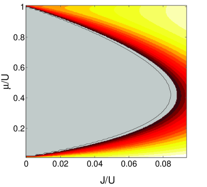
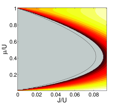
Figure 2: Plot of the zero-temperature phase diagram for $\Delta_{\max}=0.1$(upper panel) and $\Delta_{\max}=0.2$ (lower panel). In black we have plotted the border between the MI and the BG phase, while the colored background corresponds to the superfluid fraction (grey=$0$). It is possible to notice how the BG phase covers an increasing area as $\Delta_{\max}$ is increased.

III Stability of the Mott phase

In the present Section we introduce a procedure to determine the border of the MI phase which is based on the stability of the self-consistency map induced by the mean-field procedure.

As a first consideration, it is possible to state that the condition $\gamma_{k}=0$ for every $k$ corresponds to the gapped insulating phase of the mean-field Hamiltonian 3. Indeed, in this case the local ground-states (7) are eigenvectors of the local number operator $a^{\dagger}a$

$$|\psi\rangle=|n\rangle=\frac{(a^{\dagger})^{n}}{n!}|0\rangle,\quad n=\lceil\frac{\mu}{U}\rceil,$$ (12)

where $\lceil x\rceil$ denotes the smallest integer larger than $x$, and hence the mean-field ground-state (7) is a pure Fock state. As for the ordered Bose-Hubbard Hamiltonian, the relevant on-site energy is

$$\epsilon_{n}=\frac{U}{2}n(n-1)+\mu n$$ (13)

Hence $\langle\psi|a|\psi\rangle=0$ at every site, and the self-consistency constraint (8) is satisfied. In other terms $\gamma_{k}=0$ is a fixed point of the map defined by Eq. (8). The gapped insulating phase is stable as long as this fixed point is stable. This is true as long as the magnitude of the maximal eigenvalue of the matrix $\Lambda$ appearing in the linearized version of Eq.(8) is smaller than 1, see (14). In order to determine $\Lambda$, we assume $|\gamma_{k}|\ll 1$ and consider the (mean-field) kinetic term in Hamiltonian (4) as perturbative. If first order perturbation theory is performed one gets

$$\langle a_{m}\rangle=\frac{J}{U}F\left(\frac{\mu}{U}\right)\sum_{m^{\prime}}A_{m\,m^{\prime}}\langle a_{m^{\prime}}\rangle$$ (14)

where

$$F\left(x\right)=\frac{x+1}{(\lceil x\rceil-x)(x-\lfloor x\rfloor)}$$ (15)

Hence the linearized version of the self-consistency map Eq. (8) can be written as

$$\langle a_{m}\rangle=\frac{J}{U}\sum_{m^{\prime}}\Lambda_{m\,m^{\prime}}\langle a_{m^{\prime}}\rangle$$ (16)

where the matrix $\Lambda$ is proportional to the adjacency matrix $A$:

$$\Lambda=F\left(\frac{\mu}{U}\right)A.$$ (17)

Recalling the criteria for the stability of linear maps, the fixed point $\langle a_{m}\rangle=0$ (equivalent to $\gamma_{m}=0$) is stable whenever

$$\frac{J}{U}\leq\frac{1}{|\tilde{\lambda}_{\max}|}$$ (18)

where $\tilde{\lambda}_{\max}$ the eigenvalue of $\Lambda$ with the largest magnitude.

The problem of determining the maximal eigenvalue of the matrix $\Lambda$ can be reduced to the calculation of the maximal eigenvalue of the ( tridiagonal ) adjacency matrix $A$. Note that $A$ is basically the one-particle Hamiltonian for a non-interacting off-diagonal Anderson model (random hopping model). If $\lambda_{\max}$ is the maximal eigenvalue of the adjacency matrix, Eq. (18) can be recast as

$$\frac{J}{U}\leq\frac{1}{|\lambda_{\max}|F\left(\frac{\mu}{U}\right)}.$$ (19)

We have dealt with the calculation of the eigenvalues of $A$ both numerically and analytically. The analytical approach consists in the determination of the spectral density of the matrix, given the probability distribution of the elements of the matrix following the approach outlined by Dyson for and harmonic-oscillator chain A:Dyson , while the former simply consists in the direct numerical evaluation of the matrix eigenvalues.

III.1 Numerical analysis

In Fig. 3 we report the maximum eigenvalue $\lambda_{\max}$ for the random adjacency matrix $A$ as a function of the strength of disorder for both a single realization and a disorder average over 1000 samples. The two panels refer to different lattice sizes. In every case, it is evident that the maximal eigenvalue $\lambda_{\max}$ grows with increasing disorder strength, $\Delta_{\max}$ .

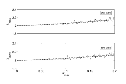
Figure 3: $\Delta_{\max}$-dependence of the largest eigenvalue of the adjacency matrix $A$, for 200 sites (upper panel) and 100 sites (lower panel). By comparison between the single realization plots (full lines) and the averaged ones (dashed lines),it is possible to see how, increasing the lattice size, the effect of the specific randomness realization is decreased

The stability condition given by Eq. (19), along with the above considerations about the $\lambda_{\max}$-dependence from $\Delta_{\max}$ are in agreement with the considerations of Section II.1 , as far as the MI phase is concerned. In particular $\lambda_{\max}$ can be thought of as a shrinking factor for the MI lobe when compared to a homogeneous situation.

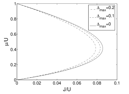
Figure 4: Boundary of the MI region for different values of $\Delta_{\max}$.

III.2 Analytical solution

In this section we would like to describe an analytical method to obtain the largest eigenvalue of a (possibly infinite) random adjacency matrix whose entries are given by Eq. (9). For some particular disorder distributions it is possible to carry through the analytical calculation and, as a consequence, solve Eq. (19) without finite-size effects.

It is worth mentioning that, in principle, the information gained through this approach is richer. In fact for some specific realizations of disorder it is possible to obtain the full integrated density of states $M(z)$ and not simply the largest eigenvalue of the adjacency matrix.

The solution of the problem can be obtained following the approach proposed by Dyson for the solution of a linear chain of harmonic oscillators.

Here we will sketch Dyson’s approach, outlining the connection with our problem, providing the portion of $M(z)$ needed to obtain the largest eigenvalue in view of Eq. (19).

In A:Dyson , the problem of a linear harmonic chain with springs of random elastic is reformulated as a tridiagonal matrix diagonalization problem. The matrix $\Lambda$ has the following form

$$\Lambda_{J+1,J}=-\Lambda_{J,J+1}=i\lambda_{J}^{1/2}$$ (20)

which is related to the matrix $A$ defined in Eq. (5) by a unitary transformation $U(\theta)$

$$U_{J,K}(\theta)=\delta_{J,K}\exp(i\theta J)$$ (21)

with

$$\Lambda=U(\theta)\,A\,U(\theta)$$ (22)

and

$$\theta=\frac{\pi}{2}-\phi$$

and setting $s_{J}=\lambda_{J}^{1/2}$ in Eq. (5). The unitarity of $U(\theta)$ allows to state that the eigenvalues of $\Lambda$ are equal to the eigenvalues of $A$, hence the procedure followed in A:Dyson can be directly mapped onto our problem.

The core of this approach resides in the definition of the characteristic function of the chain

$$\Omega(x)=\lim_{N\rightarrow\infty}\frac{\sum_{j}\log(1+x\omega_{j}^{2})}{N}$$ (23)

where $N$ is the size of the matrix, and $\omega_{j}$ the desired eigenvalues of the matrix under consideration.

The density of states $D(z)$ and the integrated density of states

$$M(z)=\int_{0}^{z}D(z^{\prime})dz^{\prime}$$

can be obtained from the characteristic function through the following relation

$$D(z)=-\frac{1}{z^{2}\pi}{\rm Im}\left[\lim_{\epsilon\rightarrow 0}\Omega^{\prime}(-\frac{1}{z}+i\epsilon)\right]$$ (24)

having defined

$$\Omega^{\prime}(x)=\frac{d\Omega}{dx}.$$

The determination of $\Omega(x)$ is obtained through a power series expansion

$$\Omega(x)=\lim_{N\rightarrow\infty}\frac{1}{N}\sum_{n=1}^{\infty}(-1)^{n-1}Tr(\Lambda^{2n}).$$ (25)

The determination of $Tr(\Lambda^{2n})$ leads to the following relation

$$\Omega(x)=\lim_{N\rightarrow\infty}\frac{1}{N}\sum_{a=1}^{N}\log\left[1+\xi(a)\right]$$ (26)

having defined $\xi(a)$ through the continued fraction

$$\xi(a)=x\lambda_{a}/\left(1+x\lambda_{a+1}/\left(1+x\lambda_{a+2}/\left(\dots\,\right.\right.\right..$$ (27)

If, as it may be safely assumed in our case, the various values of $\lambda_{a}$ are independent random variables with probability distribution $G(\lambda)$, the variable

$$\xi(a)=\frac{x\lambda_{a}}{1+\xi(a+1)}$$

will have probability distribution $F(\xi)$ satisfying the following integral equation

$$F(\xi)=\int_{0}^{\infty}F(\xi^{\prime})G\left[\xi(1+\xi^{\prime}/x)\right]\frac{1+\xi^{\prime}}{x}d\xi^{\prime}.$$ (28)

With the normalization condition

$$\int_{0}^{\infty}F(\xi)d\xi=1$$ (29)

we obtain

$$\Omega(x)=2\int_{0}^{\infty}F(\xi)\log(1+\xi)d\xi.$$ (30)

If we assume a Poissonian form for $G(\lambda)$

$$G_{n}(\lambda)=\frac{n^{n}}{(n-1)!}\lambda^{n-1}\exp(-n\lambda),$$ (31)

Eq. (28) has an analytical solution. Hence it is possible to obtain the integrated density of states in closed form in terms of integral functions.

The integrated density of states for $A$ can be simply obtained back by posing

$$M^{A}(z)=M(z^{2})$$ (32)

since in A:Dyson $M(z)$ is defined as the proportion of eigenvalues for which $\omega_{j}^{2}<z$, while $M^{A}(z)$ as the proportion of eigenvalues with $\lvert\omega_{j}\rvert<z$. As a simple check, we provide here the expression for $M^{A}_{\infty}(z)$, corresponding to the case without disorder, i.e. $n=\infty$ in Eq. (31),

$$\begin{array}[]{lll}M^{A}_{\infty}(z)&=\frac{1}{\pi}\arccos\left[1-1/2z^{2}\right]&z<2\\ &=1&z>2.\end{array}$$ (33)

which, as expected, coincides with the well known result for a 1D homogeneous system.

On the other hand, if we are interested in the determination of the maximal eigenvalue of $A$ in presence of (weak) disorder whose distribution can be related to that expressed by Eq. (31), we can consider a large-$n$ expansion of $M^{A}_{n}(z)$ for $z>2$. The expression of $M^{A}_{n}$ in this case is given by

$$M^{A}_{n}(z)\simeq 1-\frac{\alpha}{\pi}\exp\left[-\alpha-2n\left(\sinh\alpha-\alpha\right)\right]$$ (34)

with $\alpha=\textrm{arccosh}\left(1/2z^{2}-1\right)$.

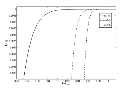
Figure 5: Comparison between three analytical solutions for $M(Z)=1$, it is possible to see how, for decreasing disorder ($n$ increasing) the solution approaches the solution of the problem without randomness. In the $x$-axis the variable $z$ has been normalized with respect to the maximum eigenvalue $\lambda_{max}$

Fig. 5 shows the behavior of the integrated density of states in the vicinity of the band edge at $\lambda_{\max}$, for three different values of the disorder strength. In Ref. A:Buonsante06CM the behavior of the corresponding density of states is related to the presence of a BG phase outside the MI region. In that case a possible direct transition from the MI to the SF phase is possible for small disorders and specific values of the chemical potential, and signaled by a singularity at the band edge in the density of states, similar to the Van Hove singularity characterizing the homogeneous case, Eq. (33). Conversely, in the present case, where density of states depends on the chemical potential through an overall multiplicative factor, an infinitesimal disorder is sufficient to smear the discontinuity in the density of states. Hence an intermediate BG phase is expected for every value of the chemical potential, which is in agreement with the previously noted shape of the BG phase in Figs. 2and 4.

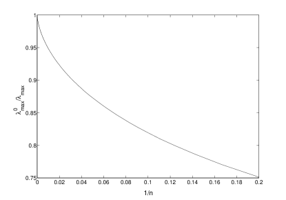
Figure 6: Plot of the “shrinking factor” for the MI lobe boundary as a function of the disorder intensity ($1/n\rightarrow 0$ represents the case without disorder).

IV Conclusions

In this paper we have considered the effect of a random hopping term on the zero-temperature phase diagram of the Bose-Hubbard Hamiltonian. Analogously to what happens when a random on-site term is considered, we have observed the emergence of a Bose-glass phase. The analysis has been performed within a mean-field approach both numerically and analytically. The boundaries of the Mott lobes and the presence of a surrounding BG phase has been related to the spectral feature of an off-diagonal Anderson model. For the future, we plan to extend our research towards the finite-temperature case and to higher dimensions.

Acknowledgments. One of the authors (PB) acknowledges a grant form Lagrange project-CRT Foundation and hospitality of the Ultra Cold Atoms group at the University of Otago. The work of F.M. has been entirely supported by the MURST project Cooperative Phenomena in Coherent System of Condensed Matter and their Realization in Atomic Chip Devices.

References

- (1) D. Jaksch and P. Zoller, Ann. Phys. 315, 52 (2005).
- (2) M. P. A. Fisher, P. B. Weichman, G. Grinstein and D. S. Fisher, Phys. Rev. B 40, 546 (1989).
- (3) J. E. Lye, L. Fallani, M. Modugno, D. S. Wiersma, C. Fort and M. Inguscio, Phys. Rev. Lett. 95, 070401 (2005); D. Clement, A. F. Varon, M. Hugbart, J. A. Retter, P. Bouyer, L. Sanchez-Palencia, D. M. Gangardt, G. V. Shlyapnikov and A. Aspect, ibid., 170409; C. Fort, L. Fallani, V. Guarrera, J. E. Lye, M. Modugno, D. S. Wiersma and M. Inguscio, ibid., 170410;
- (4) R. Roth, Phys. Rev. A 68, 023604 (2003).
- (5) B. Damski, J. Zakrzewski, L. Santos, P. Zoller and M. Lewenstein, Phys. Rev. Lett. 91, 080403 (2003). T. Schulte, S. Drenkelforth, J. Kruse, W. Ertmer, J. Arlt, K. Sacha, J. Zakrzewski and M. Lewenstein,ibid., 170411.
- (6) L. Fallani, J. E. Lye, V. Guarrera, C. Fort and M. Inguscio, cond-mat/0603655 .
- (7) M. Wallin, E. S. Sørensen, S. M. Girvin and A. P. Young, Phys. Rev. B 49, 12115 (1994); M. B. Hastings, ibid. 64, 024517 (2001); R. Graham and A. Pelster, cond-mat/0508306 (2005).
- (8) B. V. Svistunov, Phys. Rev. B 54, 16131 (1996).
- (9) F. Pázmándi and G. T. Zimányi, Phys. Rev. B 57, 5044 (1998).
- (10) K. Sheshadri, H. R. Krishnamurthy, R. Pandit and T. V. Ramakrishnan, Euorphys. Lett. 22 (1993).
- (11) W. Krauth, M. Caffarel and J.-P. Bouchaud, Phys. Rev. B 45, 3137 (1992).
- (12) K. Sheshadri, H. R. Krishnamurthy, R. Pandit and T. V. Ramakrishnan, Phys. Rev. Lett. 75, 4075 (1995).
- (13) K. V. Krutitsky, P. A. and G. R., New J. Phys. 8, 187 (2006).
- (14) R. T. Scalettar, G. G. Batrouni and G. T. Zimanyi, Phys. Rev. Lett. 66, 3144 (1991); W. Krauth, N. Trivedi and D. Ceperley, ibid. 67, 2307 (1991); G. G. Batrouni and R. T. Scalettar, Phys. Rev. B 46, 9051 (1992); J. Kisker and H. Rieger, ibid. 55, R11981 (1997); P. Hitchcock and E. S. Sorensen, ibid. 73, 174523 (2006);
- (15) J.-W. Lee and M.-C. Cha, Phys. Rev. B 70, 052513 (2004).
- (16) K. G. Singh and D. S. Rokhsar, Phys. Rev. B 49, 9013 (1994); A. D. Martino, M. Thorwart, R. Egger and R. Graham, Phys. Rev. Lett. 94, 060402 (2005).
- (17) J. K. Freericks and H. Monien, Phys. Rev. B 53, 2691 (1996).
- (18) R. V. Pai, R. Pandit, H. R. Krishnamurthy and S. Ramasesha, Phys. Rev. Lett. 76, 2937 (1996).
- (19) S. Rapsch, U. Schöllwock and W. Zwerger, Europhys. Lett. 46, 559 (1999).
- (20) R. Pugatch, N. Bar-Gill, N. Katz, E. Rowen and N. Davidson, cond-mat/0603571 (2006); P. Louis and M. Tsubota, cond-mat/0609195 (2006).
- (21) P. Buonsante, V. Penna, A. Vezzani and P. Blakie, cond-mat/0610476 (2006).
- (22) O. Penrose and L. Onsager, Phys. Rev. 104, 576 (1956).
- (23) S. Sachdev, Quantum Phase Transitions (Cambridge University Press, Cambridge, UK, 1999) (1999).
- (24) D. van Oosten, P. van der Straten and H. T. C. Stoof, Phys. Rev. A 63, 053601 (2001).
- (25) A. S. Ferreira and M. A. Continentino, Phys. Rev. B 66, 014525 (2002).
- (26) J.-B. Bru and T. Dorlas, J. Stat. Phys. 113, 177 (2004).
- (27) P. Buonsante and A. Vezzani, Phys. Rev. A 70, 033608 (2004).
- (28) A. Rey, K. Burnett, R. Roth, M. Edwards, C. Williams and C. Clark, J. Phys B 36, 825 (1993).
- (29) P. Buonsante, V. Penna and A. Vezzani 70, 061603(R) (2004).
- (30) P. Buonsante, V. Penna and A. Vezzani, Las. Phys. 15, 361 (2005).
- (31) F. J. Dyson, Phys. Rev. 92, 1331 (1953).