Study of the Magnetic Film Materials by Horizontal Scanning Mode for the Magnetic Force Microscopy in Magnetostatic and ac Regimes.

Abstract

The magnetic force microscopy inverse problem for the case of horizontal scanning of a tip on a linear magnetic film is introduced. We show the possibility to recover the magnetic permeability of the material from the experimental data by using the Hankel (Fourier-Bessel) transform inverse method (HIM). This method is applied to the case of a layered slab film as well. The inverse problem related to the ac MFM is introduced.

I Introduction

In the theory of inverse magnetic force microscopy (MFM), the recovering of the magnetic permeability is based on the interaction of a tip with the stray field of a magnetic material. So far the inverse problem has been solved in magnetostatic considerations for different cases such as sphericalcoffeyprb1 , seminfinitecoffeyinverse and slabdelacruzPhysB04 geometries. In order to measure the magnetostatic interaction force, the direction of the MFM tip movement has been always assumed to be perpendicular to the surface of the sample.

This vertical movement mode of the MFM entails a mathematical procedure based on the Laplace transform inverse method (LIM)badiaprb99 ; badiaprb01 ; coffeyotherinver ; coffeyprl ; coffeyprb98 applied to experimental data. Solutions of the LIM are not unique since the numerical Laplace transform inversion is intrinsically unstablebadiaprb01 ; coffeyprb0 . In other words, small variations in the initial conditions or the noise present in the experimental data cause large variations of results.

In this paper, we assume lateral displacements of the tip which allow us to consider the use of the Hankel transform inverse method (HIM)artobadia , an alternative approach to LIM, for recovering the magnetic permeability $\mu_{r}$. We first present the inverse problem related to the MFM for a finite magnetic slab. We extend the proposed Hankel inverse algorithm to the case of a finite layered film and recover the magnetic properties as well as the geometrical characteristics of each layer.

Finally, we introduce the HIM for the $ac$ MFM regime to study a magnetic slab.

II Slab film magnetostatic inverse problem

Let us consider the tip as a magnetic point dipole $\vec{m}$ with components $(0,0,m_{z})$ placed at the position $(0,0,a)$ outside a magnetic slab film of thickness $b$. The film is located at $z=0$ parallel to the $xy$ plane. We assume the relative magnetic permeability $\mu_{r}=\mu/\mu_{0}$ of the material to be constant, where $\mu_{0}$ is the magnetic permeability in the vacuum. The scalar potential $\phi$ satisfies the Poisson equation

$$\nabla^{2}\phi=\vec{m}\cdot\vec{\nabla}\delta(x)\,\delta(y)\,\delta(z-a).$$ (1)

The general solution $\phi$ of the Poisson equation is given by a sum of a particular solution $\phi_{1}$ and a homogeneous solution $\phi_{2}$. This decomposition of $\phi$ corresponds to the decomposition of the induction $\vec{B}(\vec{r})$ (where $\vec{B}(\vec{r})=-\mu_{0}\vec{\nabla}\phi$), into the sum $\vec{B}(\vec{r})=\vec{B}_{1}(\vec{r})+\vec{B}_{2}(\vec{r})$, where $\vec{B}_{1}(\vec{r})$ represents the direct magnetic field induction due to the dipole, and $\vec{B}_{2}(\vec{r})$ is the reflected magnetic induction.

For the dipole $\vec{m}$, we have

$$\phi_{1}(\vec{r})=\,\frac{\mu_{0}}{4\pi}\,\frac{\vec{m}\cdot\vec{r}}{{|\vec{r}_{1}|^{3}}},$$ (2)

where $\vec{r}_{1}\equiv(x,y,z-a)$.

Now, we expand $\phi_{1}(\vec{r})$ in terms of the Bessel functions. For that we use the following identity

$$\frac{1}{\sqrt{\rho^{2}+z^{2}}}=\int_{0}^{\infty}dk\,e^{-k|z|}\,J_{0}(k\rho).$$ (3)

Here and throughout, $J_{\ell}$ denotes the Bessel function of $\ell^{th}$ order of the first kind and $\rho^{2}=x^{2}+y^{2}$ . Eq.(3) and the recurrence relations of Bessel functions permit us to express the $z$-component of $\phi_{1}(\vec{r})$ from Eq.(2) in the followingdelacruzPhysB04 compact form,

$$\phi_{z1}=\frac{m_{z}}{4\pi}\int_{0}^{\infty}dk\,e^{-k(z-a)}\,k\,J_{0}(k\rho).$$ (4)

The distribution of the magnetic field induction $\vec{B}(\vec{r})$ is given by

$$\vec{B}(\vec{r})=\left\{\begin{array}[]{l}\vec{B}_{1}(\vec{r})+\vec{B}_{2}(\vec{r})\qquad z>0\\ \vec{B}_{3}(\vec{r})\qquad\qquad-b<z<0\\ \vec{B}_{4}(\vec{r})\qquad\qquad\qquad z<-b\;,\\ \end{array}\right.$$ (8)

where $\vec{B}_{3}(\vec{r})$ and $\vec{B}_{4}(\vec{r})$ are the penetrating and transmitted magnetic fields respectively.

The following governing elliptic differential equations hold for $\vec{B}(\vec{r})$

$$\nabla^{2}\vec{B}_{i}(\vec{r})=0,\,\,(i=1,\ldots,4).$$ (9)

Then, analogous to Eq.(4), we can write the $z$-component of the scalar potentialsdelacruzPhysB04 as follows:

$$\phi_{z2} = \frac{m_{z}}{4\pi}\int_{0}^{\infty}dkkI_{z2}(k)e^{-k(a+z)}J_{0}(k\rho),$$

$$\phi_{z3} = \frac{m_{z}}{4\pi}\int_{0}^{\infty}dkk[I_{z3}^{+}e^{kz}+I_{z3}^{-}e^{-kz}]e^{-ka}J_{0}(k\rho),$$

$$\phi_{z4} = \frac{m_{z}}{4\pi}\int_{0}^{\infty}dkkI^{+}_{z4}(k)e^{-k(a-z-b)}J_{0}(k\rho).$$ (10)

The coefficients $I_{z_{i}}(k)$ can be obtained if we impose the continuity boundary conditions on $\phi_{z_{i}}$ and $\mu\,\partial\phi_{z_{i}}/\partial z$ at the interfaces ($z=0,z=-b$). Notice that we do not consider the solutions which are divergent as $z\rightarrow\pm\infty$ for the fields $B_{z3}$ and $B_{z4}$. We are interested in the coefficient $I_{z_{2}}(k)$ since $B_{z2}$ is the only magnetic field that interacts with the tip. For this coefficient we have from Eq.(II)

$$I_{z2}(\mu_{r},k) = \Delta_{\mu}\,(e^{2bk}-1)\,(1-\mu_{r}^{2}),$$ (11)

where $\Delta_{\mu}\equiv(e^{2bk}(\mu_{r}+1)^{2}-(\mu_{r}-1)^{2})^{-1}$. The expressions for the incident, reflected, penetrating and transmitted fields respectively are

$$B_{z_{1}} = \frac{\mu_{0}\,m_{z}}{4\pi}\int_{0}^{\infty}dk\,k^{2}\,e^{-k(a-z)}J_{0}(k\rho),$$ (12)

$$B_{z_{2}} = \frac{\mu_{0}\,m_{z}}{4\pi}\int_{0}^{\infty}dk\,k^{2}\,I_{z_{2}}(\mu_{r},k)\,e^{-k(a+z)}J_{0}(k\rho),$$ (13)

$$B_{z_{3}} = \frac{\mu\,m_{z}}{4\pi}\int_{0}^{\infty}dkk^{2}[I_{z_{3}}^{+}(\mu_{r},k)e^{kz}+I_{z_{3}}^{-}(\mu_{r},k)e^{-kz}]$$ (14)

$$\times \,e^{-ka}J_{0}(k\rho),$$

$$B_{z_{4}} = \frac{\mu_{0}\,m_{z}}{4\pi}\int_{0}^{\infty}dk\,k^{2}\,I_{z_{4}}(\mu_{r},k)\,e^{-k(a-z-b)}J_{0}(k\rho).$$ (15)

The interaction force between the tip and the slab is given by

$$F_{z}(a)=-\frac{\partial}{\partial a}\,(-\frac{1}{2}\>\vec{m}\cdot\vec{B}_{2}),$$ (16)

and it can be rewritten using Eq.(13) as follows

$$F_{z}(a)=\frac{\mu_{0}m^{2}_{z}}{4\pi}\int^{\infty}_{0}\,dk\,k^{3}\,I_{z2}(\mu_{r},k)\,e^{-2a\,k}\,J_{0}(k\rho).$$ (17)

Let us assume that we need to recover the unknown $\mu_{r}$ from the MFM data (i.e. the force $F_{z}$). Consider a horizontal displacement of the tip such that the distance $a$ between the tip and the magnetic film remains constant, $a=a_{0}$.

Recalling the definition of the Hankel transform operator

$$\mbox{\Sc\char 72\relax}_{0}[f(k)](\rho)=\int kJ_{0}(k\rho)f(k)dk,$$ (18)

we can write Eq.(17) as follows

$$F_{z}(a_{0},\rho)=\frac{\mu_{0}\,m^{2}_{z}}{4\pi}\mbox{\Sc\char 72\relax}_{0}[k^{2}I_{z2}(\mu_{r},k)\,e^{-2ka_{0}}].$$ (19)

The data inversion process involved in our algorithm reduces to a simpler operation, the so-called Hankel transform inversion. The forward and inverse transformations have the same operational formartobadia $\mbox{\Sc\char 72\relax}_{0}^{-1}=\mbox{\Sc\char 72\relax}_{0}$.

Let us now describe the algorithm for finding $\mu_{r}$ starting with the experimental force data. The mathematical inversion should be performed for the pairs $[\rho_{i},F_{z}(a_{0},\rho_{i})]$ where $\rho$ is the Hankel transformed variable. We apply the inverse operator $\mbox{\Sc\char 72\relax}_{0}^{-1}$ to both sides of Eq.(19).

Consider the quantity $\mbox{\Sc\char 72\relax}_{0}^{-1}[F_{z}(a_{0},\rho)](k)$ to be known for some collection of values of the wave-number $k$. Using these data it is possible to determine the pair $(\mu_{r},b)$ or $(\mu_{r},I_{z2})$ as follows. Assuming $k$ as a parameter, we can take any nontrivial pair $k_{1}\neq k_{2}$ and write the following nonlinear system of equations:

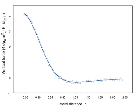
Figure 1: Plot of the simulated force $F_{z}(a_{0},\rho)$ used in this work. A noise corrupted data have been added.

$$\frac{\mathcal{T}(a_{0},k_{1})}{k^{2}_{1}}\;\mbox{\Sc\char 72\relax}_{0}^{-1}[F_{z}(a_{0},\rho)](k_{1})-{I}_{z2}(\mu_{r},k_{1}) = 0$$

$$\frac{\mathcal{T}(a_{0},k_{2})}{k^{2}_{2}}\;\mbox{\Sc\char 72\relax}_{0}^{-1}[F_{z}(a_{0},\rho)](k_{2})-{I}_{z2}(\mu_{r},k_{2}) = 0,$$ (20)

where $\mathcal{T}(a_{0},k)\equiv 4\pi{\rm e}^{2ka_{0}}/\mu_{0}m^{2}_{z}$.

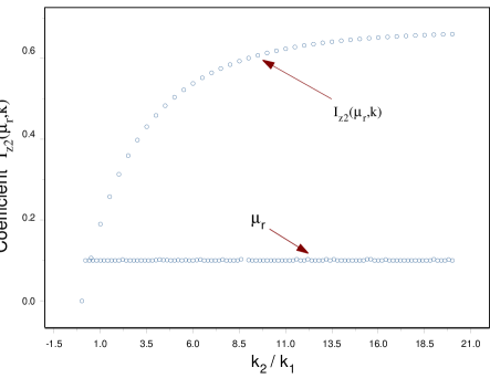
Figure 2: The magnetic permeability $\mu_{r}$ and the coefficient $I_{z2}$ recovered by using the Hankel transform technique.

The system (II) allows us to obtain the quantity $\mu_{r}$ from the force experimental data. To prove that the described method gives the value of $\mu_{r}$, we perform a simulationbadiaprb99 ; artobadia with a set of faked MFM data with $a_{0}=0.435,\,b=0.2,\,\rho=0.2$ and $\mu_{r}=0.1$. Here and throughout the paper the units are measured in $\mu m$. The corresponding graph is shown in the Fig.1.

Fig.2 displays the results of the recovering of $\mu_{r}$ and the coefficient $I_{z2}(\mu_{r},k)$. The results agree with the theoretical value of the parameter $\mu_{r}$ used in the forward problem shown in Fig.1, in a large range of values of the wave-number $k$.

III Layered film magnetostatic inverse problem

The inverse problem for the slab can be generalized in order to study the magnetic multilayered films.

Let us consider a finite slab film that geometrically can be viewed as a collection of $M$ layers. Denote the $z$-coordinate of the $j$-th layer by $z_{j}$. We say that the lowest layer is designated as layer 1, while layer $M$ is the top of the slab and $z_{M}=0$. The slab has a total thickness $z_{1}=-b$. We assume a constant magnetic permeabilities $\mu_{rj}$ $(j=1,...,M)$ to be different for each layer.

The distribution of the magnetic field $\vec{B}(\vec{r})$ can be written as

$$\vec{B}_{1}(\vec{r})+\vec{B}_{2}(\vec{r}) z>0,$$

$$\vec{B}_{3}(\vec{r}) z_{j}<z<z_{j+1},$$

$$\vec{B}_{4}(\vec{r}) z<z_{1}.$$

The elliptic differential equations $\nabla^{2}\vec{B}_{i}=0\,(i=1,\ldots,4)$ hold. The $z$-components of $\vec{B}_{2},\vec{B}_{3}$ and $\vec{B}_{4}$ are given by

$$B_{z_{2}} = \frac{\mu_{0}m_{z}}{4\pi}\int_{0}^{\infty}dkk^{2}I^{(M+1)}_{z_{2}}(k)e^{-k(a+z)}J_{0}(k\rho),$$ (22)

$$B_{z_{3}} = \frac{\mu m_{z}}{4\pi}\int_{0}^{\infty}dkk^{2}[I_{z_{3}}^{j+}(k)e^{kz}+I_{z_{3}}^{j-}(k)e^{-kz}]$$ (23)

$$\times e^{-ka}J_{0}(k\rho),$$

$$B_{z_{4}} = \frac{\mu_{0}m_{z}}{4\pi}\int_{0}^{\infty}dkk^{2}I_{z_{4}}(k)e^{-k(a-z-z_{1})}J_{0}(k\rho).$$ (24)

The coefficients $I_{z_{i}}(k)$ may be obtained by imposing continuity boundary conditions at the planar interfaces $z_{M}=0$ and $z=z_{j}$ on $B_{z_{i}}$ in a way similar to that described in section II.

Taking into account Eqs.(16) and (22), we can write the expression for the force between the tip and the layered film as follows

$$F_{z}(a)=\frac{\mu_{0}m^{2}_{z}}{4\pi}\int^{\infty}_{0}dkk^{3}I^{(M+1)}_{z2}e^{-2ak}J_{0}(k\rho).$$ (25)

Notice that $I^{(M+1)}_{z2}$ contains all the geometrical and physical information related to the layered film. This coefficient is a function of the permeability and position of each layer, i.e. $I^{(M+1)}_{z2}=I^{(M+1)}_{z2}(k,z_{j},\mu_{rj})$.

Taking into account the definition (18) of the Hankel transform $\mbox{\Sc\char 72\relax}_{0}$, we apply its inverse $\mbox{\Sc\char 72\relax}_{0}^{-1}$ to both sides of Eq.(25). For $M$ couples of values $k_{j+1}\neq k_{j}$ we get the following nonlinear system, which is analogous to (II):

$$\frac{\mathcal{T}(a_{0},k_{M+1})}{k_{M+1}^{2}}\mbox{\Sc\char 72\relax}_{0}^{-1}[F_{z}(a_{0},\rho)](k_{M+1})-I^{(M+1)}_{z2}(k_{M+1}) = 0$$

$$\cdots$$ (26)

$$\frac{\mathcal{T}(a_{0},k_{j})}{k_{j}^{2}}\mbox{\Sc\char 72\relax}_{0}^{-1}[F_{z}(a_{0},\rho)](k_{j})-I^{(M+1)}_{z2}(k_{j}) = 0.$$

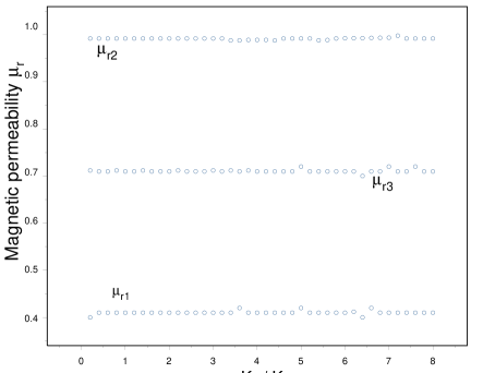
Figure 3: Recovery of the magnetic permeabilities $\mu_{r1},\mu_{r2}$ and $\mu_{r3}$ for a slab with $M$=3. The theoretical values assumed for $\mu_{rj}$ are $0.41,0.9,0.71$, respectively.

In order to get the force noise corrupted data, we have followed the simulation procedure used in section II for the slab geometry. Fig.3 shows the result of applying the described inverse method to a film having three layers.

Notice that the magnetic layered film-tip interaction problem involves an attenuating magnetic field penetrationcoffeyprb0 . If the experimental data of the force reflect this fact, then better results in the inverse procedure for layers situated next to the top of the slab $(z=0)$ can be archived.

IV $ac$ Regime for a slab film

It is well-known that one achieves better results using the MFM if one considers the $ac$ regime rather than a magnetostatic interaction between the tip and the filmbadiaprb01 . The $dc$ measurement is easily corrupted by noise, such as vibrations and $1/f$ electronic noise. Much higher sensitivity of MFM can be achieved in the $ac$ mode by driving the cantilever at its resonant frequency by that one reduces environmental noise and increases the signal to noise ratio using lock-in or frequency modulation techniqueszhugrutter . To develop and to solve the inverse problem in the case of the $ac$ regime with the inclusion of losses we follow the method developed by Badia in Ref.[badiaprb01, ].

First, let us assume the tip $(0,0,m_{z})$ to be harmonically driven at a constant height above a magnetic slab. The cantilever oscillation amplitude is considered to be constant as well. This condition is used for dissipation imaging, an imaging technique which is sensitive to non-conservative interactions zhugrutter ; grutter .

We consider a small vertical oscillation of the tip around the point located at the distance $a$ from the film. Denote by $a^{\prime}$ the distance between the tip and the film. Then we have the relation $a^{\prime}=a+A^{\prime}\cos(w_{d}t)$, where $A^{\prime}$ is the amplitude of the tip oscillations, which satisfies the condition $A^{\prime}\ll a$. The quantity $w_{d}$ is used for the driving angular frequency of the MFM tip.

Taking into account the nondispersive ohmic relation $\vec{J}=\sigma_{n}\vec{E}$ and the well-known time-dependent Maxwell equations, we get the following relation for the magnetic field inside the film $\nabla^{2}\vec{B}=\bar{\mu}\sigma_{n}\partial\vec{B}/\partial t$. The quantity $\sigma_{n}$ is the conductivity and $\bar{\mu}$ is the permeability of the material.

The relative permeability $\mu_{r}$ to be determined is related to the real part $\mu^{\prime}$ of $\bar{\mu}$ as follows: $\mu^{\prime}=\mu_{r}\mu_{0}$, where $\bar{\mu}=\{\mu^{\prime}+i\mu^{\prime\prime}\}$. Now we are going to determine $\bar{\mu}$ as a first step in order to get $\mu_{r}$. To that end, we shall find the force acting on the tip and solve the inverse problem.

Replacing $a$ by $a^{\prime}$ in (12), we get

$$B_{z1} = \frac{\mu_{0}m_{z}}{4\pi}\int_{0}^{\infty}dkk^{2}e^{-k(a-z)}J_{0}(k\rho)$$

$$- \frac{\mu_{0}m_{z}}{4\pi}A^{\prime}\cos(w_{d}t)\int_{0}^{\infty}dkk^{3}e^{-k(a-z)}J_{0}(k\rho)$$

$$+ \frac{\mu_{0}m_{z}}{8\pi}A^{\prime 2}\cos^{2}(w_{d}t)\int_{0}^{\infty}dkk^{4}e^{-k(a-z)}J_{0}(k\rho).$$

The following similar expressions can be obtained for $B_{zi}$ $(i=2,3,4)$:

$$B_{z2} = \frac{\mu_{0}m_{z}}{4\pi}\int_{0}^{\infty}dkk^{2}e^{-k(a+z)}I_{z2}(k,\mu^{\prime})J_{0}(k\rho)$$ (28)

$$- \frac{\mu_{0}m_{z}}{4\pi}A^{\prime}\cos(w_{d}t)\int_{0}^{\infty}dkk^{3}e^{-k(a+z)}I_{z2}(k,\mu^{\prime})$$

$$\times J_{0}(k\rho)+\frac{\mu_{0}m_{z}}{8\pi}A^{\prime 2}\cos^{2}(w_{d}t)\int_{0}^{\infty}dkk^{4}e^{-k(a+z)}$$

$$\times I_{z2}(k,\mu^{\prime})J_{0}(k\rho),$$

$$B_{z3} = \frac{m_{z}}{4\pi}\int_{0}^{\infty}dkk^{2}[I^{+}_{z3}(k,\mu^{\prime})e^{kz}+I^{-}_{z3}(k,\mu^{\prime})e^{kz}]e^{-ka}$$ (29)

$$\times J_{0}(k\rho)-\frac{m_{z}}{4\pi}A^{\prime}\cos(w_{d}t)\int_{0}^{\infty}dkk^{3}[I^{+}_{z3}(k,\mu^{\prime})e^{kz}$$

$$+ I^{-}_{z3}(k,\mu^{\prime})e^{kz}]e^{-ka}J_{0}(k\rho)+\frac{m_{z}}{8\pi}A^{\prime 2}\cos^{2}(w_{d}t)$$

$$\times \int_{0}^{\infty}dkk^{4}[I^{+}_{z3}(k,\mu^{\prime})e^{kz}+I^{-}_{z3}(k,\mu^{\prime})e^{kz}]$$

$$\times e^{-ka}J_{0}(k\rho),$$

$$B_{z4} = \frac{\mu_{0}m_{z}}{4\pi}\int_{0}^{\infty}dkk^{2}e^{-k(a-z-b)}I_{z4}(k,\mu^{\prime})J_{0}(k\rho)$$ (30)

$$- \frac{\mu_{0}m_{z}}{4\pi}A^{\prime}\cos(w_{d}t)\int_{0}^{\infty}dkk^{3}e^{-k(a-z-b)}I_{z4}(k,\mu^{\prime})$$

$$\times J_{0}(k\rho)+\frac{\mu_{0}m_{z}}{8\pi}A^{\prime 2}\cos^{2}(w_{d}t)\int_{0}^{\infty}dkk^{4}e^{-k(a-z-b)}$$

$$\times I_{z4}(k,\mu^{\prime})J_{0}(k\rho).$$

Notice that the coefficients $I_{zi}(k,\mu^{\prime})$(see Eq.(11)) are similar to the ones found in the magnetostatic casedelacruzPhysB04 .

In order to find the coefficients $I^{\pm}_{zi}(k,\mu^{\prime})$, we consider the following representation of the incident, reflected, penetrating and transmitted fields as $B_{zi}(t)=B^{dc}_{zi}+B^{w_{d}}_{zi}(w_{d},t)+B^{2w_{d}}_{zi}(w_{d},t)$, where $(i=1,\ldots,4)$.

Let us denote by w a formal variable which takes the values $w_{d}$ and $2w_{d}$. Assuming the notation $B^{ac}$=Re$[\tilde{B}e^{i{\textsl{w}}t}]$ and taking into account the time-independent solutions (12-15) for $B^{dc}_{zi}$ (i=2,3,4), we get the following governing differential equations

$$\nabla^{2}\tilde{B}^{\textsl{w}}_{z2}(t) = 0,$$

$$\nabla^{2}\tilde{B}^{\textsl{w}}_{z3}(t) = i2\delta^{-2}(\textsl{w})\,\tilde{B}^{\textsl{w}}_{z3}(t),$$ (31)

$$\nabla^{2}\tilde{B}^{\textsl{w}}_{z4}(t) = 0,$$

where the skin depth $\delta(\textsl{w})$ is defined by $\delta(\textsl{w})\equiv(2/\textsl{w}\,\bar{\mu}\,\sigma_{n})^{1/2}$.

We note that Eq.(IV) for $\tilde{B}^{\textsl{w}}_{3}$ is analogous the equation $\nabla^{2}\vec{B}=(1/\lambda^{2})\vec{B}$, which arises from the London equation for the superconductor ($\lambda$ is the London penetration depth).

In a similar way to Eqs.(12-15), we find solutions $B^{w_{d}}_{zi}$ and $B^{2w_{d}}_{zi}$ $(i=2,3,4)$ of system (IV) as well as $B^{dc}_{zi}$ in the form:

$$B^{dc}_{z2} = \frac{\mu_{0}m_{z}}{4\pi}\int_{0}^{\infty}dk\,k^{2}e^{-k(a+z)}I_{z2}(k,\mu^{\prime})J_{0}(k\rho)$$

$$+ \frac{\mu_{0}m_{z}}{16\pi}A^{\prime 2}\int_{0}^{\infty}dk\,k^{4}e^{-k(a+z)}I_{z2}(k,\mu^{\prime})J_{0}(k\rho),$$

$$\tilde{B}^{w_{d}}_{z2} = -\frac{\mu_{0}m_{z}}{4\pi}A^{\prime}\int_{0}^{\infty}dk\,k^{3}e^{-k(a+z)}\widetilde{{\cal I}}^{w_{d}}_{z2}(k,\mu^{\prime})J_{0}(k\rho),$$

and

$$\tilde{B}^{2w_{d}}_{z2} = \frac{\mu_{0}m_{z}}{16\pi}A^{\prime 2}\int_{0}^{\infty}dk\,k^{4}e^{-k(a+z)}\widetilde{{\cal I}}_{z2}^{2w_{d}}(k,\mu^{\prime})J_{0}(k\rho)\>.$$

The corresponding expressions for the penetrated fields are:

$$B^{dc}_{z3} = \frac{m_{z}}{4\pi}\int_{0}^{\infty}dk\,k^{2}[I_{z_{3}}^{+}(k,\mu^{\prime})e^{kz}+I_{z_{3}}^{-}(k,\mu^{\prime})e^{-kz}]$$ (35)

$$\times e^{-ka}J_{0}(k\rho)$$

$$+ \frac{m_{z}}{16\pi}A^{\prime 2}\int_{0}^{\infty}dk\,k^{4}[I_{z3}^{+}(k,\mu^{\prime})e^{kz}+I_{z3}^{-}(k,\mu^{\prime})e^{-kz}]$$

$$\times e^{-ka}J_{0}(k\rho),$$

and

$$\tilde{B}^{w_{d}}_{z3}(k,\mu^{\prime}) = -\frac{m_{z}}{4\pi}A^{\prime}\int_{0}^{\infty}dk\,k^{2}[\widetilde{{\cal I}}_{z3}^{w_{d}+}(k,\mu^{\prime})e^{kz}$$ (36)

$$+ \widetilde{{\cal I}}_{z3}^{w_{d}-}(k,\mu^{\prime})e^{-kz}]e^{-ka}J_{0}(k\rho),$$

$$\tilde{B}^{2w_{d}}_{z3}(k,\mu^{\prime}) = \frac{m_{z}}{16\pi}A^{\prime 2}\int_{0}^{\infty}dk\,k^{4}[\widetilde{{\cal I}}_{z3}^{2w_{d}+}(k,\mu^{\prime})e^{kz}$$ (37)

$$+ \widetilde{{\cal I}}_{z3}^{2w_{d}-}(k,\mu^{\prime})e^{-kz}]e^{-ka}J_{0}(k\rho),$$

and the transmitted fields are given by

$$B^{dc}_{z4}(k,\mu^{\prime}) = \frac{\mu_{0}m_{z}}{4\pi}\int_{0}^{\infty}dk\,k^{2}e^{-k(a-z-b)}I_{z4}(k,\mu^{\prime})J_{0}(k\rho)$$ (38)

$$+ \frac{\mu_{0}m_{z}}{16\pi}A^{\prime 2}\int_{0}^{\infty}dk\,k^{4}e^{-k(a-z-b)}I_{z4}(k,\mu^{\prime})$$

$$\times J_{0}(k\rho),$$

and

$$\tilde{B}^{w_{d}}_{z4}(k,\mu^{\prime}) = -\frac{\mu_{0}m_{z}}{4\pi}A^{\prime}\int_{0}^{\infty}dk\,k^{2}e^{-k(a-z-b)}\widetilde{{\cal I}}^{w_{d}}_{z4}(k,\mu^{\prime})$$ (39)

$$\times J_{0}(k\rho),$$

$$\tilde{B}^{2w_{d}}_{z4}(k,\mu^{\prime}) = \frac{\mu_{0}m_{z}}{16\pi}A^{\prime 2}\int_{0}^{\infty}dk\,k^{4}e^{-k(a-z-b)}\widetilde{{\cal I}}_{z4}^{2w_{d}}(k,\mu^{\prime})$$ (40)

$$\times J_{0}(k\rho).$$

To obtain the coefficients $\widetilde{{\cal I}}^{w_{d}}_{z2}(k,\mu^{\prime})$ and $\widetilde{{\cal I}}_{z2}^{2w_{d}}(k,\mu^{\prime})$, we must impose the continuity boundary conditions on each field components at the interfaces $z=0$ and $z=-b$.

Now we shall derive the time-dependent force acting on the oscillating tip. In fact, in the dipole limit, the instantaneous value of this force may be calculated from the expression ${\cal F}_{z}(t)=-\partial_{a^{\prime}}\{{-(1/2)\vec{m}\cdot\vec{B}_{2}[a^{\prime}(t)]}\}$.

The magnetic force ${\cal F}_{z}(t)$ can be decomposed into the sum ${\cal F}_{z}(t)=F^{dc}_{z}+F_{z}^{ac}(t)$. The linear approximation with respect to $A^{\prime}$ for the components of ${\cal F}_{z}(t)$ can be written as follows

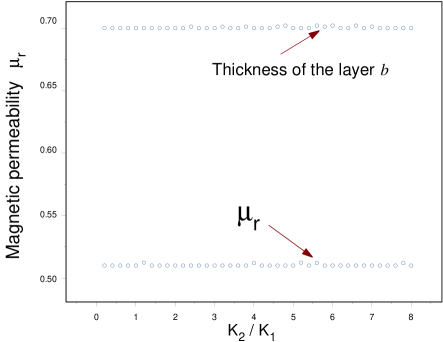
Figure 4: The graph shows the real part of the magnetic permeability $\mu_{r}$ and the thickness of the film $b$ by HIM applied to ac MFM.

$$F^{dc}_{z} = \frac{\mu_{0}m^{2}_{z}}{8\pi}\int_{0}^{\infty}dkk^{3}e^{-2ka}I_{z2}(k,\mu^{\prime})J_{0}(k\rho)$$ (41)

$$+ \frac{\mu_{0}m^{2}_{z}}{8\pi}\int_{0}^{\infty}dkk^{3}e^{-2ka}|\widetilde{{\cal I}}^{w_{d}}_{z2}|(k,\mu^{\prime})$$

$$\times J_{0}(k\rho)\cos{\varphi}^{w_{d}},$$

and

$$F^{ac}_{z} \simeq -\frac{\mu_{0}m^{2}_{z}}{8\pi}\int_{0}^{\infty}dk\,k^{4}e^{-2ka}{I}_{z2}(k,\mu^{\prime})J_{0}(k\rho)$$ (42)

$$\times A^{\prime}\cos({w_{d}t})$$

$$- \frac{\mu_{0}m^{2}_{z}}{4\pi}\int_{0}^{\infty}dkk^{4}e^{-2ka}|\widetilde{{\cal I}}^{w_{d}}_{z2}|(k,\mu^{\prime})\,J_{0}(k\rho)$$

$$\times A^{\prime}\cos({w_{d}t+\varphi^{w_{d}}})$$

$$- \frac{\mu_{0}m^{2}_{z}}{8\pi}\int_{0}^{\infty}dkk^{4}e^{-2ka}|\widetilde{{\cal I}}^{2w_{d}}_{z2}|(k,\mu^{\prime})J_{0}(k\rho)$$

$$\times A^{\prime}\cos({2w_{d}t+\varphi^{2w_{d}}}),$$

were $\widetilde{{\cal I}}^{w_{d}}_{z2}=|\widetilde{{\cal I}}^{w_{d}}_{z2}|e^{i\varphi^{w_{d}}}$ and $\widetilde{{\cal I}}^{2w_{d}}_{z2}=|\widetilde{{\cal I}}^{2w_{d}}_{z2}|e^{i\varphi^{2w_{d}}}$ and $\varphi^{w}$ is the phase lag between the tip-sample force and the displacement of the tip.

In the lowest-order approximation to the $ac$ problem, we can assume that $\varphi^{w}$ is a small parameterbadiaprb01 .

Taking into account that the force is recovered in the form $F^{ac}_{z}=\mathrm{Re}[\tilde{F}_{z}e^{iw_{d}t}]$, we can rewrite the Eq.(42) as follows

$$\tilde{F}_{z}=-\frac{\mu_{0}A^{\prime}m^{2}_{z}}{2\pi}\int_{0}^{\infty}dkk^{4}e^{-2ka}{\cal I}_{z2}(k,\mu^{\prime},w_{d})J_{0}(k\rho),$$ (43)

where we define ${\cal I}_{z2}(k,\mu^{\prime},w_{d})\equiv(1/4)I_{z2}(k,\mu^{\prime})+(1/2)\widetilde{{\cal I}}^{w_{d}}_{z2}(k,\mu^{\prime},w_{d})+(1/4)\widetilde{{\cal I}}^{2w_{d}}_{z2}(k,\mu^{\prime},2w_{d})$.

Now, we shall recover $\mu_{r}$ and $b$ from MFM measurements in $ac$ modes. First, recall that the complex amplitude of the $ac$ force $\tilde{F}_{z}=\mathrm{Re}[\tilde{F}_{z}]+i\mathrm{Im}[\tilde{F}_{z}]$ may be experimentally found.

Here, we show that a straightforward extension of the vector inversion method to complex variables can be done. Eq.(43) can be written using the operator $\mbox{\Sc\char 72\relax}_{0}$ as follows

$$\tilde{F}_{z}(a_{0},\rho)=-\frac{\mu_{0}A^{\prime}m^{2}_{z}}{2\pi}\mbox{\Sc\char 72\relax}_{0}[k^{3}e^{-2ka_{0}}{\cal I}_{z2}(k,\mu^{\prime},w_{d})].$$ (44)

Then, we can perform the mathematical inversion for the pairs $[\rho_{i},\tilde{F}_{z}(a_{0},\rho_{i})]$. In particular, one can apply the inverse operator $\mbox{\Sc\char 72\relax}_{0}^{-1}$ to both sides of Eq.(44) and obtain the following system for any $k_{1}\neq k_{2}$

$$\frac{\mathcal{G}(k_{1})}{k_{1}^{3}}\;\mbox{\Sc\char 72\relax}_{0}^{-1}[\tilde{F}_{z}(a_{0},\rho)](k_{1})+{\cal I}_{z2}(\mu^{\prime},b;k_{1}) = 0$$

$$\frac{\mathcal{G}(k_{2})}{k_{2}^{3}}\;\mbox{\Sc\char 72\relax}_{0}^{-1}[\tilde{F}_{z}(a_{0},\rho)](k_{2})+{\cal I}_{z2}(\mu^{\prime},b;k_{2}) = 0,$$ (45)

where $\mathcal{G}(k)\equiv e^{2ka_{0}}\,{2\pi}/\mu_{0}A^{\prime}m^{2}_{z}$.

To solve the system (IV) for the quantities $(\mu_{r},b)$, we use the vector inversion procedure together with the Muller’s methodmuller . The Muller’s method can be used to find zeros of a function and can be applied to complex value functionsbadiaprb01 . This method is a generalization of the secant method in the sense that it does not require the derivative of a function.

Fig.4 displays the results of recovering the magnetic permeability and the thickness of the film. These quantities were considered constants in the process of simulation using noise corrupted fake data.

IV.1 Frequency oscillation inverse method

In this section we describe the method of solving the inverse problem in terms of the shift frequency.

It is convenient to develop the inverse method using the observed frequency shift $\triangle f$ of the oscillating cantilever rather than the magnetic force, acting on the tip. If the tip oscillation amplitude $A^{\prime}$ is small compared to the distance between the tip and the slab $a_{0}$, the relation between the gradient of the force $\partial\tilde{F}_{z}(z)/\partial z$ and $\triangle f$ is given byroseman

$$\frac{\triangle f}{f_{0}}=\frac{1}{2k_{s}}\frac{\partial\tilde{F}_{z}(z)}{\partial z},$$ (46)

where $f_{0}$ is the unperturbed resonance frequency and $k_{s}$ is the spring constant of the force sensor.

We can rewrite the expression for the force given by Eq.(43) in the form

$$\tilde{F}_{z}(z) = -\frac{\mu_{0}A^{\prime}m^{2}_{z}}{2\pi}\int_{0}^{\infty}dkk^{4}e^{-k(z+a)}{\cal I}_{z2}(k,\mu^{\prime},w_{d})$$ (47)

$$\times J_{0}(k\rho).$$

In the case of the horizontal displacement of the $z-$direction oscillating tip, Eq.(46) can be written as

$$\triangle f = \frac{\mu_{0}A^{\prime}m^{2}_{z}f_{0}}{4\pi k_{s}}\int_{0}^{\infty}dkk^{5}e^{-k(z+a)}{\cal I}_{z2}(k,\mu^{\prime},w_{d})J_{0}(k\rho).$$

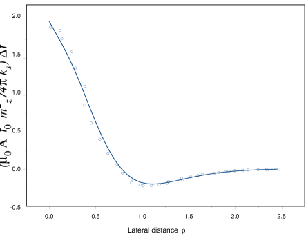
Figure 5: Plot of the simulated frequency shift $\Delta f$ versus $\rho$. A noise corrupted data have been added.

Finally, applying the operators $\mbox{\Sc\char 72\relax}_{0}$ and $\mbox{\Sc\char 72\relax}_{0}^{-1}$ to the Eq.(IV.1) and considering $z=a$ and $k$ as parameters, we get the following system of equations:

$$\frac{4\pi k_{s}f_{0}k_{i}^{4}}{\mu_{0}A^{\prime}m^{2}_{z}}\,\mbox{\Sc\char 72\relax}_{0}^{-1}[\triangle f(a)](k_{i})-{\cal I}_{z2}(k_{i},\mu^{\prime},w_{d})=0,$$ (49)

where $i=1,2$.

We have arrived to a nonlinear system analogous to (IV), but this time it is written in terms of the frequency shift $\Delta f$. The system (49) can be solved in the same way as system (IV).

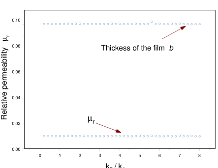
Figure 6: Plot of an example simulated force $F_{z}(a_{0},\rho)$ versus $\rho$ used in this work. A noise corrupted data have been added.

Fig.5 shows the theoretical shift frequency $\Delta f$ (continuous line) as well as a simulated measurement (symbols). The values of $a=0.8,b=0.1,\mu_{r}=0.01$ and $w_{d}=10^{3}rad/s$ were used for our faked data.

Fig.6 displays results of recovering the magnetic permeability and the thickness of the film. These quantities were considered constant in the process of simulation using noise corrupted data.

V Conclusion

Throughout this work, we have developed a theoretical background for the recovery of the magnetic permeability in magnetic films by MFM experiments. In addition, it has been shown that $b$ may be recovered from the measurements of the vertical force in the case of a horizontal scanning of the MFM tip.

Finally, we have suggested a solution of the inverse problem using the shift frequency of the system.

VI Acknowledgement

A. de la Cruz thanks to A. Badia and V. Shramshenko. This work was supported by the Department of Mathematics and Statistics and by the Physics Department of Concordia University.

References

(1)M. W. Coffey, Phys. Rev. B 60, 3346 (1999).
(2)M. W. Coffey, Inverse Problems 13, 1223 (1997).
(3)A. de la Cruz de Oña, Physica B 348, 177 (2004).
(4)A. Badía, Phys. Rev. B 60, 10436 (1999).
(5)A. Badía, Phys. Rev. B 63, 094502 (2001).
(6)M. W. Coffey, Inverse Problems 15, 669 (1999).
(7)M. W. Coffey, Phys. Rev. Lett. 83, 1648 (1999).
(8)M. W. Coffey, Phys. Rev. B 57, 11648 (1998).
(9)M. W. Coffey, Phys. Rev. B. 61, 15361 (2000).
(10)A. de la Cruz de Oña and A. Badía, Phys. Rev. B 70, 144512 (2004).
(11)X.Zhu, P.Grutter, V. Metlushko and B. Ilic, Phys. Rev. B 66, 024423 (2002).
(12)Y. Liu, B. Ellman, and P. Grutter, Appl. Phys. Lett. 71, 1418 (1997).
(13)D.E. Muller, Math. Tables Aids Comput. 10, 208 (1956).
(14)T. R. Albrecht, P. Grutter, D. Horne and D. Rugar, J. Appl. Phys. 69, 668
(1991)