LOFF and breached pairing with cold atoms

Abstract

We investigate here the Cooper pairing of fermionic atoms with mismatched fermi surfaces using a variational construct for the ground state. We determine the state for different values of the mismatch of chemical potential for weak as well as strong coupling regimes including the BCS BEC cross over region. We consider Cooper pairing with both zero and finite net momentum. Within the variational approximation for the ground state and comparing the thermodynamic potentials, we show that (i) the LOFF phase is stable in the weak coupling regime, (ii) the LOFF window is maximum on the BEC side near the Feshbach resonance and (iii) the existence of stable gapless states with a single fermi surface for negative average chemical potential on the BEC side of the Feshbach resonance.

1 Introduction

Fermionic superfluidity driven by s-wave short range interaction with mismatched fermi surfaces has attracted attention recently both theoretically gaplessth as well as experimentally gaplessexp . The experimental techniques developed during the last few years, at present, enable one to prepare atomic systems of different compositions, densities, coupling strengths as well as the sign of the coupling in a controlled manner with trapped cold fermionic atoms using techniques of Feshbach resonance expbcsbec . Because of the great flexibility of such systems, the knowledge acquired in such studies shows promise to shed light on topics outside the realm of atomic physics including dense quark matter in the interior of neutron stars quarkmatter , high $T_{c}$ superconductors htc as well as for the physics of dilute neutron gas gas .

In degenerate fermi systems, it is well known that an attractive interaction destabilizes the fermi surface. Such an instability is cured by the BCS mechanism characterized by pairing between fermions with opposite spins and opposite momenta near the fermi surface leading to a gap in the spectrum. In this system the number densities and the chemical potentials of the two condensing fermions are the same. On the other hand, there are situations where the fermi momenta of the two species that condense need not be the same. Such mismatch in fermi surfaces can be realized in different physical systems e.g. superconductor in an external magnetic field or a strong spin exchange field loff ; takada , mixture of two species of fermionic atoms with different densities and/or masses gaplessexp or charge neutral quark matter that could be there in the interior of neutron stars. The ground state of such systems shows possibilities of different phases which include the gapless superfluid phase wilczek ; rapid ; igor with the order parameter as non zero but the excitation energy becoming zero, the LOFF phase where the order parameter acquires a spatial variation loff ; loffitaly ; loffaust ; zhuang . The LOFF phase might also manifest in a crystalline structure crystal .

When the mismatch in chemical potential is small as compared to the superfluid gap, the superfluid state does not support the gapless single particle excitations. When the chemical potential difference is large as compared to the superfluid gap there could be possibility of breached pairing superfluidity wilczek ; rapid , where there are two fermi surfaces with the single particle excitation vanishing at two values of the momentum. When the mass difference between the two species is large it could also lead to interior gap superfluidity where the quasi particle excitation vanishes at a single momentum silotri . The stability of such configurations has been studied demanding positivity of the Meissner masses zhuang ; rischkeshov as well as the number susceptibilityandreas . Such an analysis has also been done for relativistic fermions with four fermi interactions rischkeshov . In these analyses the ground state was not considered explicitly. Instead, the chemical potential and the gap functions were treated as parameters, with the whole parameter space being analyzed systematically for stability criteria which were related to different possible quasi particle dispersions rischkeshov ; andreas .

Our approach to such problems has been variational with an explicit construct for the ground state rapid ; hmspm ; hmparikh ; amhma ; amhmb . The minimization of the thermodynamic potential with respect to the functions used to describe the ground state decides which phase would be favored at what density and/or coupling. This has been applied to quark matter with charge neutrality condition amhma ; amhmb ; amhmc as well as to the systems of cold fermionic atoms rapid . In the present paper we would like to extend the method to have the ansatz state general enough to include the LOFF state with a fixed momentum for the condensate. Thus our approach will be complementary to that of Ref.andreas in the sense that we shall use explicit state and solve the gap equation to determine gap function. Comparison of thermodynamic potential for different phases after the gap equation is solved will decide which phase will be favored at what coupling, density and the mismatch in fermi momentum. We also take the analysis further as compared to that in Ref.andreas to include the LOFF state, with a single plane wave.

For the case of vanishing mismatch in chemical potentials of the pairing species, a functional integral formulation with a saddle point approximation was considered to describe the crossover from BCS to Bose superfluidity randeria ; marini . A systematic analysis of the effect of gaussian fluctuations around the saddle point solution was also performed. It was shown that while the corrections from the fluctuations are extremely important for temperatures close to the critical temperature, particularly for strong coupling, the same is very small for all couplings for temperatures small compared to the critical temperature. The ability of this saddle point solution which at first sight might have been expected to work only for small couplings, to reproduce the strong coupling Bose limit is reassuring. This gives some confidence in its validity for intermediate coupling results where no obvious small expansion parameter is known randeria . As we shall show in the following, the results arising from our ansatz for the symmetric case of equal chemical potentials corresponds to this saddle point solution.

We organize the paper as follows. In section 2, we briefly introduce the model and the discuss the ansatz for the ground state. In subsection 2.1, we compute the expectation value of the Hamiltonian with respect to the ansatz state to calculate the thermodynamic potential. Minimizing the thermodynamic potential, we determine the ansatz functions in the ground state and the resulting superfluid gap equations. In section 3, we first discuss various possible phases and the corresponding results of the present investigation. Finally, we summarize and conclude in section 4.

2 The ansatz for the ground state

To discuss the superfluidity for fermionic atoms, we consider a system of two species of non-relativistic fermions with chemical potentials $\mu_{1}$ and $\mu_{2}$ and having equal masses. These two species can e.g. be the two hyperfine states of ${}^{40}Ca$. Further we shall assume a point like interaction between the two species. The Hamiltonian density is given as

$${\cal H}({\bf{r}})=\psi_{a}({\bf{r}})^{\dagger}(-\frac{{\bf{\nabla}}^{2}}{2m}-\mu_{a})\psi_{a}({\bf{r}})+g\psi^{\dagger}_{1}({\bf{r}})\psi_{1}({\bf{r}})\psi_{2}({\bf{r}})^{\dagger}\psi_{2}({\bf{r}})$$ (1)

where, $\psi^{a}({\bf{r}})$ is the annihilation operator of the fermion species ‘$a$’, and, $g$ is the strength of interaction between the two species of the fermionic atoms. Throughout the paper we shall work in the units of $\hbar=c=k_{B}=1$.

While considering Cooper pairing between fermions with different fermi momenta, it was realized by Larkin - Ovchinnikov and Fulde- Ferrel (LOFF), that it could be favorable to have Cooper pairing with nonzero total momentum unlike the usual BCS pairing of fermions with equal and opposite momentum. We shall examine here whether an ansatz with a condensate of Cooper pair of fermions having momenta ${\bf{k}}+{\bf{q}}/2$ and $-{\bf{k}}+{\bf{q}}/2$, thus with a nonzero net momentum ${\bf{q}}$ of each pair is favored over either BCS condensate or the normal state without condensates. Here, our notation is such that ${\bf{k}}$ specifies a particular Cooper pair while ${\bf{q}}$ is a fixed vector, the same for all pairs which characterizes a given LOFF state. Here the magnitude of the momentum $|{\bf{q}}|$ shall be determined by minimizing the thermodynamic potential while the direction is chosen spontaneously.

With this in mind, to consider the ground state for this system of fermionic atoms with mismatched fermi surfaces ($\mu_{1}\neq\mu_{2}$), we take the following ansatz for the ground state as

$$|\Omega\rangle={\cal U}_{q}|vac\rangle$$ (2)

where, $|vac\rangle$ is annihilated by $\psi_{r}({\bf{r}})$ and the unitary operator ${\cal U}_{q}$ is given as

$${\cal U}_{q}=\exp\left(\int\psi^{a}({\bf{k}}+\frac{{\bf{q}}}{2})^{\dagger}\psi^{b}(-{\bf{k}}+\frac{{\bf{q}}}{2})^{\dagger}\epsilon_{ab}f({\bf{k}})d{\bf{k}}-{\rm{h.c.}}\right).$$ (3)

In the above, ${\bf{k}}$ identifies a fermionic pair and each pair in the condensate has the same net momentum ${\bf{q}}$. The function $f({\bf{k}})$ is a variational function to be determined through the minimization of the thermodynamic potential. In the limit of zero net momentum (${\bf{q}}={\bf{0}}$) this ansatz reduces to the BCS ansatz considered earlier rapid ; amhmb ; amhmc . Such an ansatz breaks translational and rotational invariance. In position space, as we shall show that it describes a condensate which varies as a plane wave with wave vector ${\bf{q}}$. To include the effect of temperature and density we write down the state at finite temperature and density, $|\Omega(\beta,\mu)\rangle$, taking a thermal Bogoliubov transformation over the state $|\Omega\rangle$ using thermofield dynamics (TFD) method as tfd ; amph4

$$|\Omega(\beta,\mu)\rangle={\cal U}_{\beta,\mu}|\Omega\rangle={\cal U}_{\beta,\mu}{\cal U}_{q}|0\rangle,$$ (4)

where ${\cal U}_{\beta,\mu}$ is given as

$${\cal U}_{\beta,\mu}=e^{{\cal B}^{\dagger}(\beta,\mu)-{\cal B}(\beta,\mu)},$$ (5)

with

$${\cal B}^{\dagger}(\beta,\mu)=\int\Big{[}{\psi^{\prime}}^{a}({\bf{k}})^{\dagger}\theta_{-}^{a}({\bf{k}},\beta,\mu){{\underline{\psi}}^{\prime}}^{a}(-{\bf{k}})^{\dagger}\Big{]}d{\bf{k}}.$$ (6)

In Eq.(6) the ansatz functions $\theta_{-}^{a}({\bf{k}},\beta,\mu)$, as we shall see later, are related to the distribution function for the $a$-th species of fermions, and, the underlined operators are the operators in the extended Hilbert space associated with thermal doubling in TFD method. All the functions in the ansatz in Eq.(4), the condensate function $f({\bf{k}})$, the distribution functions $\theta^{i}({\bf{k}},\beta,\mu)$ are obtained by the minimization of the thermodynamic potential. We shall carry out this minimization in the next subsection.

2.1 Evaluation of thermodynamic potential and the gap equation

Having presented the trial state Eq.(4), we now proceed to minimize the expectation value of the thermodynamic potential with respect to the variational functions $f({\bf{k}})$, $\theta^{a}({\bf{k}},\beta)$ in the ansatz. Using the fact that, the variational ansatz state in Eq.(4) arises from successive Bogoliubov transformations, one can calculate the expectation values of various operators. In particular, for the condensate we have

$$\langle\Omega(\beta,\mu)|\psi^{a}({\bf{r}})\psi^{b}({\bf{r}})|\Omega(\beta,\mu)\rangle$$

$$=\frac{\epsilon^{ab}\exp(i{\bf{q}}\cdot{\bf{r}})}{2(2\pi)^{3}}\int\sin 2f\left({\bf{k}}-\frac{{\bf{q}}}{2}\right)$$

$$\times\left[\sin^{2}\theta^{b}(-{\bf{k}}+{\bf{q}})-\cos^{2}\theta^{a}({\bf{k}})\right]d{\bf{k}}$$

$$\equiv\epsilon^{ab}\exp(i{\bf{q}}\cdot r)I_{q},$$ (7)

which for nonzero $I_{q}$ describes a plane wave with a wave vector ${\bf{q}}$. Once one has demonstrated the instability to formation of a single plane wave, it is natural to expect that the state which actually develops has a crystalline structure. LOFF, in fact, argued the favored configuration to be a crystalline condensate which varies in space like a one dimensional standing wave $\cos({\bf{q}}\cdot{\bf{r}})$ with the condensate vanishing at the nodal planes. Which crystal structure will be free energetically most favored is still to be resolved. The present variational ansatz Eq.(4) is a first step in this direction to decide which crystalline structure will finally be chosen through minimization of the thermodynamic potential.

Similarly the number operator expectation value for the atoms of species ‘a’ is given as

$$\rho^{a} = \langle\Omega(\beta,\mu)|\psi^{a}({\bf{r}})^{\dagger}\psi^{a}({\bf{r}})|\Omega(\beta,\mu)\rangle$$ (8)

$$= \frac{1}{(2\pi)^{3}}\int\big{[}\cos^{2}f({\bf{k}}-\frac{{\bf{q}}}{2})\sin^{2}\theta^{a}({\bf{k}})$$

$$+ |\epsilon^{ab}|\sin^{2}f({\bf{k}}-\frac{{\bf{q}}}{2})\cos^{2}\theta^{b}(-{\bf{k}}+{\bf{q}})\big{]}d{\bf{k}},$$

which is independent of the space coordinate ${\bf{r}}$.

Using Eq.s (7) and (8) it is straightforward to calculate the expectation value of the Hamiltonian given in Eq.(1). We obtain

$$\epsilon\equiv\langle\Omega(\beta,\mu)|{\cal H}|\Omega(\beta,\mu)$$

$$=\frac{1}{(2\pi)^{3}}\int d{\bf{k}}\bigg{[}\left(\epsilon({\bf{k}}+\frac{q}{2})-\mu_{1}\right)$$

$$\bigg{(}\cos^{2}f({\bf{k}})\sin^{2}\theta_{1}({\bf{k}}+\frac{{\bf{q}}}{2})+\sin^{2}f({\bf{k}})\cos^{2}\theta_{2}(-{\bf{k}}+\frac{{\bf{q}}}{2})\bigg{)}$$

$$+\left(\epsilon(-{\bf{k}}+\frac{q}{2})-\mu_{2}\right)$$

$$\bigg{(}\cos^{2}f({\bf{k}})\sin^{2}\theta_{2}(-{\bf{k}}+\frac{{\bf{q}}}{2})\sin^{2}f({\bf{k}})\cos^{2}\theta_{1}({\bf{k}}+\frac{{\bf{q}}}{2})\bigg{)}\bigg{]}$$

$$+gI_{q}^{2}+g\rho_{1}\rho_{2}$$ (9)

where, the first term arises from the expectation value of the kinetic part of the Hamiltonian and the last two terms arise from the four point contact interaction term. Here, $\epsilon({\bf{k}})={\bf{k}}^{2}/(2m)$, and, the quantities $I_{q}$, $\rho^{a}$ ($a=1,2$) are defined in Eq. (7) and Eq. (8) respectively. The thermodynamic potential is given as

$$\Omega=\epsilon-\mu_{a}\rho^{a}-\frac{1}{\beta}s$$ (10)

where, we have denoted $s$ as the total entropy density of the two species given as tfd ; caldas

$$s=-\frac{1}{(2\pi)^{3}}\sum_{a}\int d{\bf{k}}\left(\sin^{2}\theta^{a}\ln(\sin^{2}\theta^{a})+\cos^{2}\theta^{a}\ln(\cos^{2}\theta^{a})\right).$$ (11)

We now apply the variational method to determine the condensate function $f({\bf{k}})$ in the ansatz Eq.(4), by requiring that the thermodynamic potential is minimized : $\partial\Omega/\partial f({\bf{k}})=0$. Such a functional minimization leads to

$$\tan 2f({\bf{k}})=\frac{gI_{q}}{\bar{\epsilon}_{q}-\bar{\nu}}\equiv\frac{\Delta}{\bar{\xi}_{q}}$$ (12)

In the above, $\bar{\epsilon}_{q}=(\epsilon({\bf{k}}+\frac{{\bf{q}}}{2})+\epsilon(-{\bf{k}}+\frac{{\bf{q}}}{2}))/2=({\bf{k}}^{2}+{\bf{q}}^{2}/4)/(2m)$ is the average kinetic energy of the two condensing fermions. Similarly, $\bar{\nu}=(\nu_{1}+\nu_{2})/2$, is the average of the interacting chemical potential of the two fermions with $\nu^{a}=\mu^{a}-g\rho^{a}$ and $\bar{\xi}_{q}=\bar{\epsilon}_{q}-\bar{\nu}$. Further, we have defined $\Delta=-gI_{q}$, with, $I_{q}$ as defined in Eq.(7). It is thus seen that the condensate function depends upon the average energy and the average chemical potential of the fermions that condense. Substituting the solutions for the condensate functions given in Eq. (12) in the expression for $I_{q}$ in Eq.(7), we have the superfluid gap equation given by

$$\Delta = -\frac{g}{(2\pi)^{3}}\int{d{\bf{k}}}\frac{\Delta}{2\bar{\omega}_{q}}\bigg{[}1-\sin^{2}\theta_{1}({\bf{k}}+\frac{{\bf{q}}}{2})$$ (13)

$$- \sin^{2}\theta(-{\bf{k}}+\frac{{\bf{q}}}{2})\bigg{]}$$

In the above, $\bar{\omega}_{q}=\sqrt{\Delta^{2}+\bar{\xi}_{q}^{2}}$ and the thermal functions $\theta^{a}({\bf{k}},\beta)$ are still to be determined.

The minimization of the thermodynamic potential with respect to the thermal functions $\theta_{a}({\bf{k}})$ gives

$$\sin^{2}\theta_{a}=\frac{1}{\exp(\beta\omega_{a})+1},$$ (14)

with the quasi particle energies given as $\omega_{1}({\bf{k}}+\frac{{\bf{q}}}{2})=\bar{\omega}_{q}+\delta_{\xi}$, and $\omega_{2}(-{\bf{k}}+\frac{{\bf{q}}}{2})=\bar{\omega}_{q}-\delta_{\xi}$, with $\delta_{\xi}\equiv(\xi_{1}-\xi_{2})/2=(\epsilon({\bf{k}}+\frac{{\bf{q}}}{2})-\epsilon(-{\bf{k}}+\frac{{\bf{q}}}{2}))/2-(\nu_{1}-\nu_{2})/2\equiv\delta_{\epsilon}-\delta_{\nu}$. It is clear from the dispersion relations that it is possible to have zero modes, i.e., $\omega^{a}=0$ depending upon the values of $\delta_{\epsilon}$ and $\delta_{\nu}$. So, although we shall have nonzero order parameter $\Delta$, there can be fermionic zero modes, the so called gapless superconducting phase abrikosov ; krischprl .

Now using these dispersion relations, and the superfluid gap equation (Eq.(13)), the thermodynamic potential (Eq.(10)) becomes

$$\Omega = \frac{1}{(2\pi)^{3}}\int d{\bf{k}}\bigg{[}(\bar{\xi}_{q}-\bar{\omega})$$ (15)

$$- \frac{1}{\beta}\sum_{a}\ln\left(1+\exp(-\beta\omega_{a})\right)\bigg{]}-\frac{\Delta^{2}}{g}$$

In what follows we shall concentrate on the case for zero temperature. In that case the distribution functions, Eq.(14) become $\Theta$ - functions i.e. $\sin^{2}\theta^{a}=\Theta(-\omega_{a})$. Further, using the identity $\lim_{a\rightarrow\infty}\ln(1+\exp(-ax)/a=-x\Theta(-x)$, in Eq. (15), the zero temperature thermodynamic potential becomes

$$\Omega = \frac{1}{(2\pi)^{3}}\int d{\bf{k}}(\bar{\xi}_{q}-\bar{\omega})$$ (16)

$$+ \frac{1}{(2\pi)^{3}}\int d{\bf{k}}\left[\omega_{1}\Theta(-\omega_{1})+\omega_{2}\Theta(-\omega_{2})\right]-\frac{\Delta^{2}}{g}.$$

To compare the thermodynamic potential with respect to the normal matter, we need to subtract out the zero gap and zero momentum (${\bf{q}}={\bf{0}}$) part from the thermodynamic potential given in Eq. (16). This is given as

$$\bar{\Omega} \equiv \Omega({\bf{q}},\Delta,\delta)-\Omega({\bf{q}}={\bf{0}},\Delta=0,\delta)$$ (17)

$$= \frac{1}{(2\pi)^{3}}\int d{\bf{k}}\left(|\bar{\xi}_{q}|-\bar{\omega}\right)$$

$$+ \frac{1}{(2\pi)^{3}}\int d{\bf{k}}\left[\omega_{1}\Theta\left(-\omega_{1}\right)+\omega_{2}\Theta\left(-\omega_{2}\right)\right]$$

$$- \frac{1}{(2\pi)^{3}}\int d{\bf{k}}(\xi-\delta_{\nu})\Theta(\delta_{\nu}-\xi)-\frac{\Delta^{2}}{g},$$

where, we have denoted $\xi={\bf{k}}^{2}/(2m)-\bar{\nu}$, the excitation energy with respect to the average fermi energy for normal matter. Further, we have assumed, without loss of generality, $\delta_{\nu}>0$. The superfluid gap in Eq.(17) satisfies the gap equation Eq.(13) which at zero temperature reduces to

$$\frac{1}{g} = -\frac{1}{(2\pi)^{3}}\int{d{\bf{k}}}\frac{1}{2\bar{\omega}_{q}}\bigg{[}1-\Theta\Big{(}-\omega_{1}({\bf{k}}+\frac{{\bf{q}}}{2})\Big{)}$$ (18)

$$- \Theta\Big{(}-\omega_{2}(-{\bf{k}}+\frac{{\bf{q}}}{2})\Big{)}\bigg{]}.$$

The above equation is ultraviolet divergent. The origin of this divergence lies in the point like four fermion interaction which needs to be regularized. We tackle this problem by defining the regularized coupling in terms of the s-wave scattering length $a_{s}$ as was done in Ref. randeria ; heiselberg to access the strong coupling regime rapid ; rupak by subtracting out the zero temperature and zero density contribution. The regularized gap equation is then given as

$$-\frac{1}{g_{R}} \equiv \frac{M}{4\pi a_{s}}$$ (19)

$$= \frac{1}{(2\pi)^{3}}\int d{\bf{k}}\bigg{[}\frac{1-\Theta(-\omega_{1})\Theta(-\omega_{2})}{2\bar{\omega}_{q}}$$

$$- \frac{1}{2\epsilon(k)}\bigg{]}$$

Using Eq.(18)and Eq.(19) in Eq.(17) to eliminate $g$ in favor of $g_{R}$, one can obtain

$$\bar{\Omega} = \frac{1}{(2\pi)^{3}}\int d{\bf{k}}\left(|\bar{\xi}_{q}|-\bar{\omega}_{q}+\frac{\Delta^{2}}{2\bar{\omega}_{q}}\right)$$ (20)

$$+ \frac{1}{(2\pi)^{3}}\int d{\bf{k}}\left[(\omega_{1}-\frac{\Delta^{2}}{2\bar{\omega}_{q}})\Theta(-\omega_{1})+(\omega_{2}-\frac{\Delta^{2}}{2\bar{\omega}_{q}})\Theta(-\omega_{2})\right]$$

$$- \frac{1}{(2\pi)^{3}}\int d{\bf{k}}\bigg{(}(|\bar{\xi}_{q}|+\delta_{\xi})\Theta(-|\bar{\xi}_{q}|-\delta_{\xi})$$

$$+ (|\bar{\xi}_{q}|-\delta_{\xi})\Theta(-|\xi_{q}|+\delta_{\xi})\bigg{)}d{\bf{k}},$$

where, $|\bar{\xi}_{q}|=({\bf{k}}^{2}+{\bf{q}}^{2}/4)/2m-\bar{\nu}$ and $\delta_{\xi}={\bf{k}}\cdot{\bf{q}}/2m-\delta_{\nu}$. We might note here that the thermodynamic potential difference as in Eq.(20) is cut-off independent and is finite. The only other quantities needed to calculate the thermodynamic potential in Eq.(20) are the chemical potentials: the average chemical potential of the two species $\bar{\nu}=(\nu_{1}+\nu_{2})/2$ and their difference $\delta_{\nu}=(\bar{\nu}_{1}-\bar{\nu}_{2})$. These two quantities can be fixed from the average number densities as

$$\bar{\rho}=\frac{1}{2}(\langle\psi_{1}^{\dagger}\psi_{1}\rangle+\langle\psi_{2}^{\dagger}\psi_{2}\rangle)$$

$$=\frac{1}{2}\frac{1}{(2\pi)^{3}}\int d{\bf{k}}\left(1-\frac{\bar{\xi}_{q}}{\bar{\omega}_{q}}\right)(1-\Theta(-\omega_{1})-\Theta(-\omega_{2})),$$ (21)

and the difference in number densities

$$\delta_{\rho} = \frac{1}{2}(\langle\psi_{1}^{\dagger}\psi_{1}\rangle-\langle\psi_{2}^{\dagger}\psi_{2}\rangle)$$ (22)

$$= \frac{1}{2}\frac{1}{(2\pi)^{3}}\int d{\bf{k}}\left(\Theta(-\omega_{1})-\Theta(-\omega_{2})\right),$$

which does not depend on the condensate function explicitly. In the following we shall discuss which phase is thermodynamically favorable at what density as the chemical potential difference is varied for a given coupling and a given average density.

For numerical calculations, it is convenient to write the Eq.s (19–22) in terms of dimensionless quantities. Thus we make the substitutions $|{\bf{k}}|=k_{f}x$, ${\bf{q}}=k_{f}{\bf{y}}$, $\Delta=\epsilon_{f}z$, $\bar{\nu}=\epsilon_{f}\nu$, $\delta_{\nu}=\epsilon_{f}\delta$, where, $k_{f}$ is the average fermi momentum and $\epsilon_{f}$ is the corresponding fermi energy. In terms of these dimensionless variables, the gap equation Eq.(19) reduces to

$$-\frac{1}{8\pi k_{f}a} = \frac{1}{4\pi^{2}}\int_{0}^{\infty}dxx^{2}\left(\frac{1}{\sqrt{(x^{2}+y^{2}/4-\nu)^{2}+z^{2}}}-\frac{1}{x^{2}}\right)$$ (23)

$$- \frac{1}{4\pi^{2}}\int_{0}^{\infty}dxx^{2}\frac{1}{2\sqrt{(x^{2}-\nu)^{2}+z^{2}}}$$

$$\times \int_{-1}^{1}dt(\Theta(-\hat{\omega}_{1})+\Theta(-\hat{\omega}_{2})).$$

Here, the quasi particle energies $\hat{\omega}_{a}$ ($a=1,2$) in units of average fermi energy are

$$\hat{\omega}_{1}=\hat{\omega}_{y}+xyt-\delta,\quad\omega_{2}=\hat{\omega}_{y}-xyt+\delta$$ (24)

where, $\hat{\omega}_{y}=\sqrt{(x^{2}+y^{2}/4-\nu)^{2}+z^{2}}$, where, $\nu$ is the average of the excitation energies of the two quasi particles in units of fermi energy. Further, in Eq.(23), the integration variable $t=\cos\theta$ and, we have chosen the momentum ${\bf{q}}$ of the condensate to be in the z- direction.

Similarly, the average density equation Eq.(21), in units of $\kappa_{f}^{3}/6\pi^{2}$, reduces to

$$1 = \frac{3}{2}\int_{0}^{\infty}dxx^{2}\int_{-1}^{1}dt\frac{1}{2}\bigg{[}(1-\frac{\xi_{y}}{\hat{\omega}_{y}})$$ (25)

$$+ \frac{\xi_{y}}{\hat{\omega}_{y}}(\Theta(-\hat{\omega}_{1})+\Theta(-\hat{\omega}_{2}))\bigg{]}.$$

Finally, the thermodynamic potential difference between the condensed phase and the normal phase can be expressed in terms of these dimensionless variables as

$$\bar{\Omega}=\frac{\epsilon_{f}\kappa_{f}^{3}}{2\pi^{2}}\bigg{[}\int x^{2}dx\left(|x^{2}-\nu+\frac{y^{2}}{4}|-\hat{\omega}_{y}+\frac{z^{2}}{2\hat{\omega}_{y}}\right)$$

$$+\int x^{2}dx\frac{dt}{2}\left((\hat{\omega}_{1}-\frac{z^{2}}{2\hat{\omega}_{y}})\Theta(-\hat{\omega}_{1})+(\hat{\omega}_{2}-\frac{z^{2}}{2\hat{\omega}_{y}})\Theta(-\hat{\omega}_{2})\right)$$

$$-\frac{1}{2}\int x^{2}dxdt\bigg{(}(|\xi_{y}|+\delta_{\xi_{y}}\theta(-\delta_{\xi_{y}}-\xi_{y})$$

$$+(|\xi_{y}|-\delta_{\xi_{y}})\theta(\delta_{\xi_{y}}-\xi_{y})\bigg{)}\bigg{]}$$

$$\equiv\frac{\epsilon_{f}\kappa_{f}^{3}}{2\pi^{2}}\bigg{[}I_{y1}+I_{y2}-I_{y3}\bigg{]},$$ (26)

where, $\delta_{\xi_{y}}=xyt-\delta$ and $I_{yi}(i=1,2,3)$ are the three integrals in the above equation. Eq.s (23), (25) and Eq.(26) will form the basis for our numerical investigation to decide regarding the phase structure. Before going to the numerical evaluations let us discuss the different phases.

3 Results

3.1 Homogeneous symmetric phase

Let us first discuss the symmetric homogeneous phase corresponding to vanishing chemical potential difference ($\delta_{\nu}=0$). In that case the renormalized gap equation, Eq.(23), reduces to the usual BCS gap equation rapid ; randeria

$$-\frac{1}{8\pi k_{f}a} = \frac{1}{4\pi^{2}}\int_{0}^{\infty}dxx^{2}\left(\frac{1}{\sqrt{(x^{2}-\nu)^{2}+z^{2}}}-\frac{1}{x^{2}}\right)$$ (27)

$$= I_{z}$$

and, the number density equation, Eq.(25), becomes

$$1 = \frac{3}{2}\int_{0}^{\infty}dxx^{2}\left(1-\frac{x^{2}-\nu}{\sqrt{(x^{2}-\nu)^{2}+z^{2}}}\right)$$ (28)

$$= I_{\rho}$$

where, $z$ and $\nu$ are respectively the superfluid gap and average chemical potential in units of fermi energy.

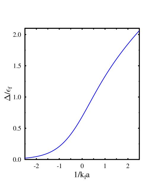
Figure 1: Superfluid gap as a function of coupling $1/k_{f}a$. The expoential rise of the gap in the BCS side ($k_{f}a<0$) is as expected from weak coupling results.

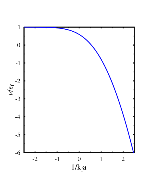
Figure 2: Self consistent solution for the chemical potential in units of fermi energy as a function of coupling $1/k_{f}a$.

It is easy to show, via integration by parts, that the integrals $I_{z}$ and $I_{\rho}$ can be rewritten as

$$I_{z}=\frac{1}{2\pi^{2}}\left(\nu I(\nu,z)-z^{2}J(\nu,z)\right)$$ (29)

and

$$I_{\rho}=z^{2}\left(I(\nu,z)+\nu J(\nu,z)\right)$$ (30)

where, we have defined the integrals $I(\nu,z)$ and $J(\nu,z)$ as

$$I(\nu,z)=\frac{1}{2}\int_{0}^{\infty}\frac{dx}{\omega(x)}$$ (31)

and

$$J(\nu,z)=\int_{0}^{\infty}\frac{x^{2}dx}{\omega(x)^{3}}$$ (32)

with $\omega(x)=\sqrt{(x^{2}-\nu)^{2}+z^{2}}$

The nice thing about these integrals $I(\nu,z)$ and $J(\nu,z)$ is that they can be expressed in terms of elliptic integrals marini . They can be written as

$$I(\nu,z)=\frac{1}{2(\nu^{2}+z^{2})^{1/4}}F(\pi/2,\kappa)$$ (33)

and

$$J(\nu,z) = \frac{(z^{2}+\nu^{2})^{1/4}}{z^{2}}E(\pi/2,\kappa)$$ (34)

$$- \frac{F(\pi/2,k)}{2(z^{2}+\nu^{2})^{1/4}(\nu+\sqrt{z^{2}+\nu^{2}})}$$

where, $F(\frac{\pi}{2},\kappa)$ and $E(\frac{\pi}{2},\kappa)$ are the elliptic integrals of first kind and second kind respectively. In the above,
$\kappa^{2}=(\nu+\sqrt{z^{2}+\nu^{2}})/(2\sqrt{z^{2}+\nu^{2}})$. The thermodynamic potential difference Eq.(26) reduces to

$$\bar{\Omega}(\delta=0,z) = \frac{\epsilon_{f}k_{f}^{3}}{2\pi^{2}}\int dxx^{2}\left(|x^{2}-\nu|-\hat{\omega}+\frac{z^{2}}{2\hat{\omega}}\right)$$ (35)

where, $\hat{\omega}=\sqrt{(x^{2}-\nu)^{2}+z^{2}}$.

In figures 1 and 2 we plot the superfluid gap and the chemical potential as functions of coupling $1/k_{f}a$ obtained by solving the coupled gap equation (Eq.(27)) and number density equations (Eq.(28)). In the weak coupling BCS limit ($1/(k_{f}a)\rightarrow-\infty$), we have $\nu>>z$ and the modulus parameter $\kappa^{2}\simeq 1-z^{2}/(4\nu^{2})$ is close to unity in the argument of the elliptic integrals. Expanding the elliptic integrals in this limit, the gap equation Eq.(29) reduces to

$$\frac{1}{8\pi k_{f}a}=-\frac{\sqrt{\nu}}{4\pi^{2}}\left(\ln\frac{8\nu}{z}-2\right).$$ (36)

This leads to the weak coupling BCS limit for the gap as $z=8e^{-2}\exp(-\pi/(|k_{f}a|))$ in units of fermi energy. Similarly in the BEC limit ($1/(k_{f}a)\rightarrow\infty$), one expects tightly bound pairs with binding energy $E_{b}=1/(ma^{2})$ and nondegenerate fermions with a large negative chemical potential randeria . In this limit $\kappa^{2}\simeq z/(4\nu^{2})<<1$. Taking this asymptotic limit of the elliptic integrals, the chemical potential $\nu$ is half of the pair binding energy. The corresponding gap is $z=(16/\pi)^{1/2}/\sqrt{k_{f}a}$ .

As may be seen from Fig. 2, the chemical potential changes sign at $\kappa_{f}a\sim 0.56$ signaling the onset of the BEC phase. Near to the unitary limit e.g. for $k_{f}a=0.01$, the ratio of condensate to the chemical potential turns out to be $\Delta/\nu=1.195$, while the chemical potential itself is numerically evaluated to be $\nu/\epsilon_{f}=0.58$. While the ratio of gap to the chemical potential $\Delta/\nu$ is very close to the value $\Delta/\nu=1.2$ obtained through quantum Monte Carlo simulations, the value of the ratio of chemical potential to the fermi energy, $\nu/\epsilon_{f}$, is higher as compared to the value $\nu/\epsilon_{f}=0.42$ obtained from quantum Monte Carlo simulation reddy . Such results arising from the variational calculations may be compared with the corresponding values obtained from other nonperturbative calculations like $\epsilon$- expansion son which turn out to be $\Delta/\nu\sim 1.31$ and $\nu/\epsilon_{f}=0.475$. We might note here that, a systematic analysis of the gaussian fluctuation around the saddle point approximation was considered in Ref. randeria . The corrections to the saddle point approximation were seen to be small for temperatures small compared to the critical temperature, for all couplings randeria .

3.2 Isotropic superfluid with mismatch in chemical potentials

With a nonzero mismatch between chemical potentials i.e. $\delta_{\nu}\neq 0$, let us consider superfluidity with a homogeneous condensate i.e. condensate with momentum ${\bf{q}}={\bf{0}}$. In that case the dispersion relations (in dimensionless variables) of the quasi particles (Eq.(24)) are given as

$$\hat{\omega}_{1}=\sqrt{(x^{2}-\nu)^{2}+z^{2}}+\delta;\quad\hat{\omega}_{2}=\sqrt{(x^{2}-\nu)^{2}+z^{2}}-\delta.$$ (37)

where, $\nu$, $z$ and $\delta$ are respectively the average chemical potential, the gap and the difference in chemical potentials in units of fermi energy.

For any value of the (dimensionless) gap $z>0$, the average chemical potential $\nu$ and the difference in chemical potentials $\delta>0$, the excitation branch $\omega_{1}$ has no zeros similar to the case of a usual superconductor. The quasi particles at the fermi surface have finite excitation energy given by the gap that is enhanced here by the mismatch $\delta$. On the other hand, the excitation branch $\omega_{2}$ can become zero depending upon the value of the gap $z$, the average chemical potential $\nu$ and the mismatch parameter $\delta$. Indeed, solving for the zeros for $\omega_{2}$ one obtains that $\omega_{2}$ vanishes at momenta (in units of fermi momentum), $x^{2}_{max/min}=\nu\pm\sqrt{\delta^{2}-z^{2}}$. Clearly, this has no solution for $\delta<z$. Further, for the case of $\delta>z$, there will be no solutions if the average chemical potential $\nu$ is smaller than $-\sqrt{\delta^{2}-z^{2}}$ since both $x_{max}^{2}$ and $x_{min}^{2}$ will become negative. On the other hand, if $\delta>z$ and $-\sqrt{\delta^{2}-z^{2}}<\bar{\nu}<\sqrt{\delta^{2}-z^{2}}$, then the expression for $x_{max}^{2}$ is positive while that of $x_{min}^{2}$ is negative. Thus there is only one zero for $\omega_{2}$. This case will correspond to ‘interior gap’ solution, where, the unpaired fermions of the first species occupy the entire effective fermi sphere. Finally, when $x^{2}_{max}>0$ and $x^{2}_{min}>0$, there are two zeros for $\omega_{2}$. This will correspond to breached pairing case where unpaired fermions of first species occupy the states between the two fermi spheres decided by $x_{max}$ and $x_{min}$.

With nonzero mismatch in the chemical potential, the gap equation for the homogeneous phase is given as

$$-\frac{1}{8\pi k_{f}a} = \frac{1}{4\pi^{2}}\int dxx^{2}\left(\frac{1}{\bar{\omega}(x)}-\frac{1}{x^{2}}\right)$$ (38)

$$- \frac{1}{4\pi^{2}}\int_{x_{min}}^{x_{max}}x^{2}\frac{1}{\bar{\omega}(x)}dx$$

$$\equiv I_{z}-I_{\delta}$$

Here, we have introduced the notation $\bar{\omega}(x)=$$\sqrt{(x^{2}-\nu)^{2}+z^{2}}$ as the average of the quasi particle energies of the two species with $\nu$ as the average chemical potential in units of fermi energy.

Further, the thermodynamic potential of Eq. (26) reduces for homogeneous condensates to,

$$\bar{\Omega}=\frac{\epsilon_{f}\kappa_{f}^{3}}{2\pi^{2}}\bigg{[}\int x^{2}dx\left(|x^{2}-\nu|-\bar{\omega}(x)+\frac{z^{2}}{2\bar{\omega}}\right)$$

$$+\int x^{2}dx\left((\omega_{1}-\frac{z^{2}}{2\bar{\omega}(x)})\Theta(-\omega_{1})\right)$$

$$-\int x^{2}dx\Theta(\delta-|x^{2}-\nu|)(|x^{2}-\nu|-\delta).\bigg{]}$$

$$\equiv\frac{\epsilon_{f}k_{f}^{3}}{2\pi^{2}}(I_{1}+I_{2}-I_{3}),$$ (39)

where, we have defined the three integrals appearing in Eq.(39) as $I_{1}$, $I_{2}$ and $I_{3}$ respectively. The integral $I_{3}$ can be evaluated directly as

$$I_{3} = \int x^{2}dx\Theta(\delta-|x^{2}-\nu|)(|x^{2}-\nu|-\delta)$$ (40)

$$= \frac{4}{15}\nu^{5/2}-\frac{2}{15}(\Theta(\nu_{+})\nu_{+}^{5/2}+\Theta(\nu_{-})\nu_{-}^{5/2})$$

with $\nu_{\pm}=\nu\pm\delta$.

Similarly, the integral $I_{2}$ can be rewritten as

$$I_{2} = \int x^{2}dx(\omega_{1}-\frac{z^{2}}{2\bar{\omega}(x)})\Theta(-\omega_{1})$$ (41)

$$= \int_{x_{min}}^{x_{max}}x^{2}dx\left(\bar{\omega}(x)-\delta-\frac{z^{2}}{2\bar{\omega}(x)}\right)$$

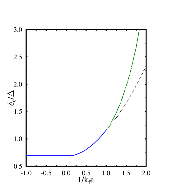
Figure 3: Ratio of critical chemical potential difference to the gap as a function of coupling strength $1/k_{f}a$. Gapless phase appears for coupling $1/k_{f}a>1$. The region between the dotted and the dashed line shows the gapless phase.

Before going to the numerical solution for the homogeneous condensates with mismatch in chemical potential, let us discuss the weak coupling BCS case. This limit is characterized by the average chemical potential being equal to the fermi energy so that $\nu=1$ and is much larger than the magnitude of both the chemical potential mismatch $\delta$ in dimensionless units and the gap $z$, also in dimensionless units. Thus this weak coupling analysis excludes the scenario with single fermi surface i.e. with the excitation energy $\omega_{2}$ having a single zero. Further, we here compare the thermodynamical potential for fixed chemical potentials. It is expected that the same analysis with fixed number densities will lead to different results – namely a mixed phase scenario which is an inhomogeneous phase where a fraction of the space is in normal phase while the remaining is in the BCS phase rupak . In this weak coupling limit, we can have ordinary superconductivity without gapless modes or can have breached pairing with $\omega_{2}$ becoming zero at two values of the momentum. The latter situation will arise for much larger values of the mismatch parameter $\delta$ as compared to the gap $z$. In the weak coupling limit, the integral $I_{1}$ becomes

$$I_{1}=\int x^{2}dx\left(|x^{2}-\nu|-\bar{\omega}(x)+\frac{z^{2}}{2\bar{\omega}}\right)\simeq-\frac{\sqrt{\nu}z^{2}}{4}$$ (42)

In the same limit, $x_{min}$=$\sqrt{\nu}=x_{max}$, so that, $I_{2}\simeq 0$. Finally, the integral $I_{3}\simeq\sqrt{\nu}\delta^{2}/4$. Thus in the weak coupling limit, the thermodynamic potential difference between the condensed and the normal phase is

$$\bar{\Omega}\simeq\frac{\epsilon_{f}k_{f}^{3}}{2\pi^{2}}(2\delta^{2}-z^{2})$$ (43)

For the ratio of the chemical potential difference to the superfluid gap $\delta/z<1/\sqrt{2}$, the Clogston–Chandrasekhar limit clog , the thermodynamic potential difference becomes negative. In this regime of $\delta/z$, the gap is the same as the $\delta=0$ gap and the density remains the same even though $\delta$ is nonzero. This critical chemical potential difference below which BCS pairing is possible depnds on the coupling strength.

In Fig.3 we plot, as a function of the coupling $1/\kappa_{f}a$, the quantity $\delta_{c}/\Delta$ the ratio of the maximum chemical potential difference to the gap that can sustain pairing. For the region below the solid and the dotted line corresponds to the parameter region where BCS pairing is the state of minimum thermodynamic potential. As may be seen from the figure, for weak coupling, the critical chmecal potential difference (in units of superfluid gap) approaches the Clogston–Chandrasekhar limit. As coupling is increased from BCS to BEC side $\delta_{c}/\Delta$ increases monotonically.

We do not find any breached pairing solutions in the BCS region with lower thermodynamic potential as compared to the normal matter. However, we do find the interior gap solution in a range of $\delta_{\nu}$ in the strong coupling BEC regime with negative average chemical potential. This happens for $1/k_{f}a>1$. This is given by the region between the dotted and the dashed line in Fig.3. In this region the density difference between the two species is also nonzero. In the region of the parameter space that is above the solid line or to the left of the dashed line is the region where no pairing is possible and the normal matter is the state of minimum thermodynamic potential.

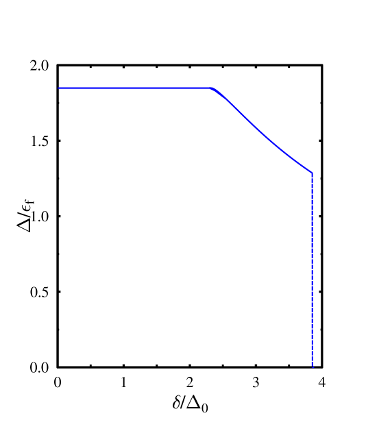
Figure 4: Superfluid gap as a function of the difference in the chemical potentials of the two species. The curve is plotted for $1/k_{f}a=2$.

In Fig.4 we plot the gap as a function of difference in chemical potential for $1/k_{f}a=2$ as a typical value for strong coupling BEC regime where gapless phase exists. In this region, the thermodynamic potential difference between the condensed phase and the normal phase is negative. The value of the gap decreases continuously from the symmetric BCS phase to the gapless phase as $\delta_{\nu}$ is increased leading to nonzero difference in the number densites. The transition from gapless phase to the normal phase which occurs at $\delta_{\nu}\simeq 3.85\Delta_{0}$ is however discontinuous. In the gapless phase the density difference between the two species is non vanishing.

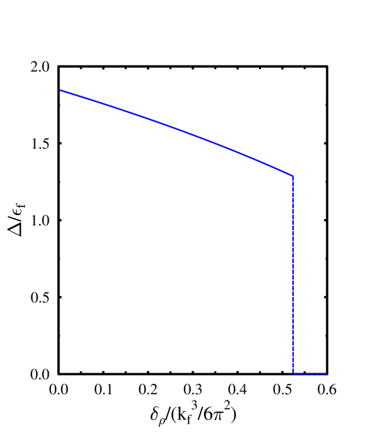
Figure 5: Superfluid gap as a function of difference in number densities of the condensing species. The curve is plotted for $1/k_{f}a=2$.

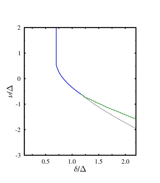
Figure 6: The ratio of average chemical potential to the gap as a function of difference of chemical potential The region between the dotted and the solid line shows the gapless phase.

As mentioned earlier, in our calculations we do not keep the difference in the densities of the two species fixed. The calculations are performed with a fixed average density and given value of chemical potential difference. In the gapless phase, the density difference comes out to be nonvanishing. In Fig.5 the dependence of the gap on the density difference $\delta_{\rho}$ is shown for the BEC region where gapless phase exists. We have taken here the value of $1/\kappa_{f}a$ as equal to 2. Superconductivity is supported for a maximum density difference of $\delta_{\rho}\simeq 0.52$ in units of $k_{f}^{3}/6\pi^{2}$ beyond which the system goes over to the normal matter with zero gap. For coupling $1/k_{f}a<1$, we do not find any superfluid phase free energetically favorable for any non zero value for the density difference, although a chemical potential difference can still support a Cooper paired BCS phase with zero net momentum..

In Fig.6, we have plotted the phase diagram in the plane of average chemical potential and the chemical potential difference, both the quantities being normalized with respect to the superfluid gap. The region above and to the right of the solid line correspond to positive thermodynamic potential and is not stable. The region below and to the left of the solid line shows Cooper pairing. The region between the dashed and the solid line shows the gapless phase. The vertical line at $\delta/\Delta=1/\sqrt{2}=0.717$ indicates the Clogston Chandrasekhar limit. These results, corresponding to explicit solutions for the gap as a function of coupling are in conformity with the results obtained in Ref. andreas .

3.3 The LOFF Phase: anisotropic superfluid with ${\bf{q}}\neq 0$

When the value of the difference in chemical potentials, $\delta$, exceeds the Clogston-Chandrasekhar limit, it can be free energetically favorable to have condensates with nonzero momentum ${\bf{q}}$, given as in Eq.(7). The dispersion relations for the quasi particles are given as

$$\omega_{1}({\bf{k}}) = \bar{\omega}({\bf{k}})+\delta_{\xi}$$ (44)

$$= \sqrt{\left(\left({\bf{k}}^{2}+\frac{{\bf{q}}^{2}}{4}\right)/2m+\bar{\nu}\right)^{2}+\Delta^{2}}$$

$$- \frac{{\bf{k}}\cdot{\bf{q}}}{2m}-\delta_{\nu}$$

$$\omega_{2}({\bf{k}}) = \bar{\omega}({\bf{k}})-\delta_{\xi}$$ (45)

$$= \sqrt{\left(\left({\bf{k}}^{2}+\frac{{\bf{q}}^{2}}{4}\right)/2m-\bar{\nu}\right)^{2}+\Delta^{2}}$$

$$+ \frac{{\bf{k}}\cdot{\bf{q}}}{2m}+\delta_{\nu}$$

The corresponding gap equation, number density equation and the thermodynamic potential are already given in Eq.s (23), (25) and (26) respectively.

As in the previous subsection, before going to discuss the detailed numerical solutions for strong couplings, let us consider the weak coupling limits of the above equations which can give an insight to the numerical solutions that can be obtained in the appropriate limit. In this limit, the average chemical potential is same as the fermi energy sothat$\sqrt{\nu}=\bar{\nu}/\epsilon_{f}\sim 1$ and is much larger than the momentum (in units of fermi momentum) $y$, gap ( in units of fermi energy) $z$ and the asymmetry in chemical potential (in units of fermi energy) , $\delta$. Further, the excitation energies in units of fermi energy can be approximated as

$$\omega_{1,2}=\bar{\omega}_{y}\pm\delta_{t}$$ (46)

where, $\bar{\omega}_{y}\simeq\sqrt{z^{2}+4\nu(x-\sqrt{\nu_{y}})^{2}}$, and, $\delta_{t}\simeq yt-\delta=\delta(\rho t-1)$, with $\rho=y/\delta$. Just to remind ourselves, $y$ is the condensate momentum in units of $k_{f}$ and $\delta$ is half of the difference in the chemical potentials of the two species in units of fermi energy $\epsilon_{f}=k_{f}^{2}/2m$. Using Eq.(36), one can eliminate the coupling $1/k_{f}a$ from the gap Eq.(23) to obtain the weak coupling LOFF gap equation as

$$\ln\left(\frac{z_{0}}{z}\right)$$

$$=\frac{\sqrt{\nu}}{2}\int dxdt\frac{1}{\bar{\omega}_{y}(x)}\left(\Theta(-\omega_{1})+\Theta(-\omega_{2})\right).$$ (47)

The theta functions in the integral above restrict the limits of $x$ integration to be in the range $(x_{min},x_{max})$,with,

$$x_{max/min}=\sqrt{\nu}\pm\frac{1}{2\sqrt{\nu}}(\delta_{t}^{2}-z^{2})^{1/2}$$ (48)

Performing the $x$-integration within the limit, the gap equation, Eq.(47), reduces to

$$\ln\left(\frac{z_{0}}{z}\right)$$

$$=\frac{1}{4}\int dt\Theta(|\delta_{t}|-z)\ln\left(\frac{|\delta_{t}|+\sqrt{\delta_{t}^{2}-z^{2}}}{|\delta_{t}|-\sqrt{\delta_{t}^{2}-z^{2}}}\right).$$ (49)

Again, the theta function restricts the angular integration where either or both the quasi particle excitation energies ($\omega_{1,2}$) become gapless. This occurs for the case when the gap $z$ is less than $(1+\rho)\delta$ as otherwise the domain of integration specified by the theta function $\Theta(|\delta_{t}|-z)$ becomes null. Depending upon the value of the gap $z$ as compared to $(\rho-1)$, either one of the two quasi particles or both become gapless ren . Using this fact, the integration over $t$ can be performed in Eq.(49) leading to the weak coupling LOFF gap equation as

$$\ln\left(\frac{z_{0}}{z}\right)$$

$$+\left[\frac{\rho+1}{4\rho}\left(\ln\frac{1-x_{1}}{1+x_{1}}+2x_{1}\right)+\frac{\rho-1}{4\rho}\left(\ln\frac{1-x_{2}}{1+x_{2}}+2x_{2}\right)\right]$$

$$=0,$$ (50)

where, $x_{1}$, $x_{2}$ are parameters

$$x_{1}=\Theta\left(1-\frac{z}{(\rho+1)\delta}\right)\left(1-\frac{z^{2}}{\delta^{2}(\rho+1)^{2}}\right)^{1/2}$$ (51)

and,

$$x_{2}=\Theta\left(1-\frac{z}{|\rho-1|\delta}\right)\left(1-\frac{z^{2}}{\delta^{2}(\rho-1)^{2}}\right)^{1/2}$$ (52)

We note here that the gap equation Eq.(50), is identical to the one derived in Ref.takada and Ref.ren for LOFF phase in the superconducting alloy with paramagnetic impurities and in quark matter respectively.

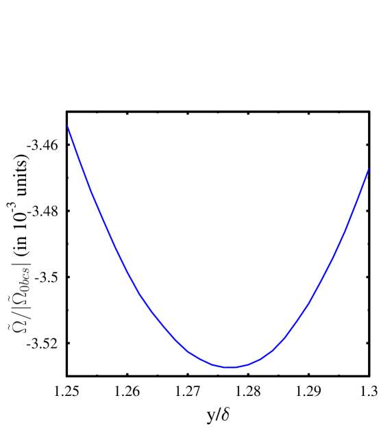
Figure 7: The thermodynamic potential between the LOFF and normal state as a function of LOFF momentum. The thermodynamic potential is normalized to the magnitude of the thermodynamic potential of the BCS state at $\delta=0$. The momentum is normalized with respect to the chemical potential difference. This curve corresponds to the value of the coupling $1/k_{f}a=-1.5$ and $\delta_{\nu}=0.72\Delta_{0}$.

Next, let us look at the thermodynamic potential Eq.(26) in the weak coupling limit. The thermodynamic potential in Eq.(26) can be written as

$$\bar{\Omega}=\frac{\epsilon_{f}k_{f}^{3}}{2\pi^{2}}\left(I_{y1}+I_{y2}-I_{y3}\right)$$ (53)

where, $I_{yi}$($i$=1,2,3) are the three integrals of Eq.(26). It is easy to show, using Eq.(42), that in the weak coupling limit

$$I_{y1}\simeq-\frac{\sqrt{(\nu-y^{2}/4)}z^{2}}{4}$$ (54)

The evaluation of the integral $I_{y2}$, is similar to the evaluation of the integral on RHS of the gap equation Eq.(47). The result is

$$I_{y2}\simeq-\frac{\sqrt{\nu}\delta^{2}}{12}\left[\frac{(\rho+1)^{3}}{\rho}x_{1}^{3}+\frac{(\rho-1)^{3}}{\rho}x_{2}^{3}\right].$$ (55)

The integral $I_{y3}$ is straightforward to evaluate and is given as

$$I_{y3} = \frac{4}{15}(\bar{\nu}-\frac{y^{2}}{4})^{5/2}-\frac{2}{15}\left((\nu+\delta)^{5/2}+(\nu-\delta)^{5/2}\right)$$ (56)

$$\simeq -\frac{\sqrt{\nu}}{2}(\nu\frac{y^{2}}{3}+\delta^{2})$$

Collecting all the terms, the thermodynamic potential Eq.(53) is given as

$$\hat{\Omega} \simeq \frac{\epsilon_{f}k_{f}^{3}}{2\pi^{2}}\frac{\sqrt{\nu}}{2}\bigg{[}\delta^{2}+\frac{y^{2}}{3}\nu-\frac{z^{2}}{2}$$ (57)

$$- \frac{\delta^{2}}{6\rho}\left((\rho+1)^{3}x_{1}^{3}+(\rho-1)^{3}x_{2}^{3}\right)\bigg{]}.$$

It is reassuring to note that the expression Eq.(57) for the thermodynamic potential is same as in Ref.takada . This is also identical to the thermodynamic potential considered for quark matter in LOFF phase in Ref.ren when degeneracy factors for the color and flavor are taken into account.

Similar to Ref. ren , it can be shown that, for the case of a small gap as compared to the chemical potential mismatch parameter, i.e. $z<<\delta$, which will be the case near a second order phase transition to normal matter, the gap is given as takada ; ren

$$z^{2}=4(\rho_{c}^{2}-1)\left(1-\frac{\delta}{\delta_{c}}\right)$$ (58)

and, the momentum $\rho=|{\bf{q}}|/\delta_{\nu}$ is given as takada ; ren

$$\rho=\rho_{c}+\frac{1}{4}\frac{\rho_{c}}{\rho_{c}^{2}-1}z^{2}.$$ (59)

In the above, $\rho_{c}$ satisfies the equation

$$\frac{1}{2\rho_{c}}\ln\frac{\rho_{c}+1}{\rho_{c}-1}=1$$ (60)

and

$$\frac{\delta_{c}}{z_{0}}=\frac{1}{2\sqrt{\rho_{c}^{2}-1}}\simeq 0.754,$$ (61)

for $\rho_{c}\simeq 1.2$.

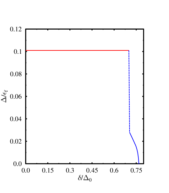
Figure 8: Superfluid gap as a function of chemical potential difference. The coupling parameter here is taken as $1/k_{f}a=-1.5$.

Here, $\delta_{c}=0.754z_{0}$ is the maximum value of the chemical potential difference that can support the LOFF phase beyond which the system goes to the normal matter phase. For a general gap parameter which need not be small as compared to the chemical potential difference, one has to solve the gap equation Eq.(50) numerically. This is done for a given value of LOFF momentum $\rho$ so that the thermodynamic potential as given in Eq.(57) is calculated for a given value of the momentum. The minimization of the thermodynamic potential numerically over the magnitude of momentum gives the best value of the LOFF momentum.

In the present calculations, however, we do not use the weak coupling gap equation, Eq.(50). Instead, for given values of coupling $1/k_{f}a$, the chemical potential difference $\delta_{\nu}$ and LOFF momentum $q$, the coupled equations Eq.(23) and Eq.(26) are solved in a self consistent manner. Using the values of the gap and the average chemical potential so obtained we calculate the thermodynamic potential using Eq.(26). For the numerical analysis, we first start with the weak coupling BCS regime $\delta_{\nu}=\delta_{max}$, the boundary that separates the LOFF phase and the normal phase. For $\delta_{\nu}<\delta_{max}$ , we solve the gap Eq. (23) for a given value of $|{\bf{q}}|$. Solution to the LOFF gap equations exist for a range of $|{\bf{q}}|$. For each value of $\delta$ we can determine the ‘best $|{\bf{q}}|$’: the choice of $|{\bf{q}}|$ that has the lowest thermodynamic potential. In Fig.7, the difference of thermodynamic potential between the LOFF phase and the normal matter is plotted as a function of the LOFF momentum for coupling $1/k_{f}a=-1.5$ and the chemical potential difference $\delta_{\nu}=0.72\Delta_{0}$. We have normalized the thermodynamic potential with respect to the magnitude of the thermodynamic potential for the BCS phase. We note here that at this value of $\delta$, which is greater than the Clogston–Chandrasekhar limit, the normal matter has lower thermodynamic potential than the homogeneous BCS phase. Thus the LOFF state is favored when the thermodynamic potential difference that is plotted in Fig.7 is negative. For weak coupling this happens when $\delta_{\nu}>0.705\Delta_{0}$, a value slightly lower than the Clogston–Chandrasekhar limit. In this region there are also other solutions of gap equation with homogeneous gap, but with higher value of the thermodynamic potential. At each $\delta<\delta_{max}$ we also compare the thermodynamic potential for the ‘best $|{\bf{q}}|$’ and that of homogeneous BCS phase. We see that for $\delta>\delta_{min}$, LOFF state has lower thermodynamic potential as compared to the homogeneous BCS phase. At $\delta_{min}$ there is a first order phase transition between the LOFF and the BCS phases. Thus in the ‘LOFF window’ $\delta_{\max}-\delta_{min}$, the LOFF state has lower energy as compared to the BCS or the normal phase. For weak coupling, our numerical values for the condensate, the momentum of the condensate and the LOFF window match with those obtained in Ref.loff ; takada .

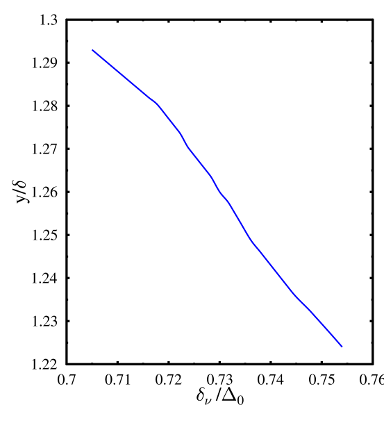
Figure 9: LOFF momentum in units of mismatch in chemical potential as a function of mismatch in chemical potential in units of gap at zero mismatch $\Delta_{0}$. The coupling here is $1/k_{f}a=-1.5.$

The variation of the gap parameter as a function of difference in chemical potential is shown in Fig. 8 for coupling $1/k_{f}a=-1.5$. Beyond $\delta_{max}$, the stress of difference in the chemical potentials leads to the vanishing of the condensate, as a second order phase transition. The variation of the LOFF momentum with respect to the chemical potential difference is shown in Fig.9. With $y=|{\bf{q}}|/k_{f}$, (${\bf{q}}$, being the LOFF momentum), we have plotted here the ratio $y/\delta$ as a function of the chemical potential difference $\delta$ which decreases monotonically from a value 1.29 at $\delta_{\nu}/\Delta_{0}=0.704$ to about 1.22 at $\delta_{\nu}/\Delta_{0}=0.754$. These values are similar to those obtained in Ref.takada ; ren in the weak coupling limit.

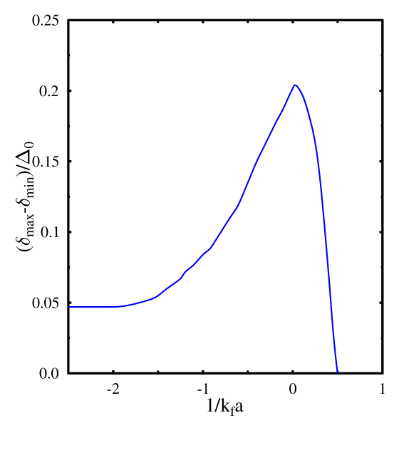
Figure 10: The LOFF window in units of the gap at zero temperature as a function of coupling $1/k_{f}a$

Next we explore how the width of the LOFF window depends upon the strength of the coupling. We see that from the weak coupling BCS side, as we increase the coupling the lower limit $\delta_{min}$ of the LOFF window decreases very slowly while the upper limit $\delta_{max}$ increases. We might note here that the thermodynamic potential difference between the LOFF state and the normal matter is very small. We had seen in the last subsection that the Clogston – Chandrasekhar limit remains almost constant in the BCS side of the Feshbach resonance (see e.g. Fig.3). $\delta_{min}$ which is very near to this value, thus is almost constant on the BCS side of Feshbach resonance. With $\delta_{max}$ increasing in this region, the LOFF window increases. However, the Clogston – Chandrasekhar limit increases with the coupling for positive scattering length and $\delta_{min}$ of the LOFF window also increases resulting in reduction of the LOFF window in the positive coupling region. Thus the LOFF window turns out to be a non monotonic function of the coupling and it becomes maximum at $1/k_{f}a\simeq 0.04$. Beyond this it decreases rapidly. For coupling greater than $1/k_{f}a=0.5$; there is no longer any window of mismatch in chemical potential in which LOFF state occurs. However, these results can be modified with a more involved ansatz of multiple plane waves as opposed to the single plane wave ansatz as considered in Eq.(3) or Eq.(7). Such multi plane wave ansatz was suggested to be favorable near the upper edge of the LOFF window crystal . In this context, it is worthwhile to mention also that the LOFF window can be considerably expanded if one considers optical latticeskoponen rather than the pairing in free space as considered here. As discussed earlier, for couplings $1/k_{f}a>1$, the the interior gap state is preferred within a certain range of mismatch in chemical potential.

4 Summary and discussions

We have considered here a variational approach to discuss the ground state structure for a system of fermionic atoms with mismatch in their fermi momenta. An explicit construct for the ground state is considered to describe two fermion condensate with nonzero momentum. The ansatz functions including the thermal distribution functions have been determined from the minimization of the thermodynamic potential. This is done for fixed chemical potentials. A similar analysis for fixed number densities leads to different results rupak .

For comparison of thermodynamic potential, we have subtracted out the free energy of normal phase (with $\Delta=0$ and ${\bf{q}}={\bf{0}}$) as in Eq.(10). This difference is finite without introducing any arbitrary cut off in the momentum zhuang . The four fermi coupling is also renormalized as in Eq.(19), by subtracting out the vacuum contribution and relating it to the s-wave scattering length as in Ref.s rapid ; randeria ; heiselberg . This makes all the quantities well defined and finite. Rewriting the gap equations and the number density equations for the symmetric case in terms of elliptic integrals as in Eqs. (29) and (30) is particularly useful regarding the numerical evaluation.

We have not calculated here the Meissner masses rischkeshov ; ren or the number susceptibility andreas to discuss stability of different phases by ruling out regions of the parameter space for the gap function and the difference in chemical potentials. Instead, we have solved the gap equations and the number density equations self consistently and have compared the thermodynamic potentials. This apart, we have also extended the analysis to incorporate the possibility of condensate with finite momentum through the the ansatz for the ground state. In certain regions of chemical potential difference and couplings we have multiple solutions for the gap equation. In such cases we have chosen the solution which has the least value for the thermodynamic potential.

In the weak coupling BCS limit we obtain the usual LOFF solution i.e. the condensate with finite momentum, in a small window of the chemical potential difference of about 0.05 times the gap at zero chemical potential difference. This LOFF window increases as the coupling is increased and becomes maximum at $1/k_{f}a\sim 0.04$ and vanishes at $1/k_{f}a=0.5$. Within the present approach we do not see any breached pairing solution being favored on the BCS side of the Feshbach resonance. However, interior gap superfluid phase with a single fermi surface appears to be possible on the strong coupling BEC side of the Feshbach resonance with negative chemical potential similar to results in Ref.andreas . The transition between BCS to LOFF phase is a first order one with the order parameter varying discontinuously at $\delta_{min}$, while the LOFF phase to normal phase transition is second order at chemical potential difference $\delta_{max}$. On the other hand, in the strong coupling BEC region, the phase transition from BCS to interior gap phase is a second order phase transition while the phase transition from interior gap phase to the normal phase is a first order phase transition as the chemical potential difference is varied.

These results are of course limited by the simplified ansatz as considered here giving a unified description for the uniform as well as spatially modulated superfluid. Similar ansatz with uniform condensates has been used earlier interpolating the BCS ($g\rightarrow 0^{+}$, $1/a\rightarrow-\infty$) and BEC ($g\rightarrow\infty$, $1/a\rightarrow\infty$) limits for the case of zero chemical potential difference randeria ; marini . The results as obtained here might nevertheless be regarded as a reference solution with which other numerical or analytical solutions obtained from more involved ansatz for the ground state can be compared.

Although the present numerical analysis has been done for zero temperature, the expressions to include temperature effects have been derived here. Clearly, the effect of fluctuations involving the corrections from the collective modes will play an important role for high temperatures particularly for the strong coupling randeria . The effect of including different masses of the two species as well as using a realistic potential for the two atomic species will be interesting regarding the study of the phase structure. Further, the study of some of the transport properties in different phases including viscosity would be very interesting for cold atomic superfluids. Some of these calculations are in progress and will be reported elsewhere amppn .

5 Acknowledgements

We would like to thank B. Deb, P.K. Panigrahi, A. Vudaygiri, D. Angom, S. Silotri, B. Chatterjee for many illuminating discussions. HM would like to thank organisers of the meeting on ’Interface of QGP and Cold atom physics ’ at ECT^∗, Trento and acknowledges discussions with D.Rischke, Y. Nishida, G.C. Strinati, P. Piere and C. Lobo during the meeting. AM would like to acknowledege financial support from Department of Science and Technology, Government of India (project no. SR/S2/HEP-21/2006).

References

- (1) W.V. Liu, F. Wilczek, Phys. Rev. Lett90, 047002 (2003); S.T. Wu and S.K. Yip, Phys. Rev. 97,053603(2003).
- (2) M.W. Zwierlein, A. Schirotzek, C.H. Schunck and W. Ketterle, Science 311, 492 (2006); G.B. Patridge, W. Li, Y. Kamer, R. LandLiao and M.W. Zwierlein, A. Schirotzek, C.H. Schunck and W. Ketterle, cond-mat/0605258.
- (3) K.M. O’hara et al, Science 298, 2179 (2002); C.A. Regal, M. Greiner and D.S. Jin, Phys. rev. Lett.92, 040403 (2004); M. Bartenstein et al, Phys. Rev. Lett.92, 120401 (2004); M.W. Zwierlein et al, Phys. Rev. Lett 92, 120403 (2004); J. Kinast et al, Phys. Rev. Lett. 92, 150402 (2004); T. Bourdel at al, Phys. Rev. Lett. 93, 050401 (2004).
- (4) For reviews see K. Rajagopal and F. Wilczek, arXiv:hep-ph/0011333; D.K. Hong, Acta Phys. Polon. B32,1253 (2001); M.G. Alford, Ann. Rev. Nucl. Part. Sci 51, 131 (2001); G. Nardulli, Riv. Nuovo Cim. 25N3, 1 (2002); S. Reddy, Acta Phys Polon.B33, 4101(2002); T. Schaefer arXiv:hep-ph/0304281; D.H. Rischke, Prog. Part. Nucl. Phys. 52, 197 (2004); H.C. Ren, arXiv:hep-ph/0404074; M. Huang, arXiv: hep-ph/0409167; I. Shovkovy, arXiv:nucl-th/0410191.
- (5) See e.g. in Q. Chen, J. Stajic, S. Tan and K. Levin, Phys Rep 412, 1 (2005) and references therein.
- (6) G. Bertsch, in Proceedings of the X conference on Recent Progress in Many-Body theories, edited by R.F. Bishop et al.(World Scientific, Singapore, 2000).
- (7) A.I. Larkin and Yu.N. Ovchinnikov, Sov. Phys. JETP20 (1965); P. Fulde and R.A. Ferrel, Phys Rev. A135, 550, 1964.
- (8) S. Takada and T. Izuyama, Prog. theor. Phys. 41, 635 (1969).
- (9) E. Gubankova, W.V. Liu, F. Wilczek, Phys. Rev. Lett. 94, 110402, (2003).
- (10) B. Deb, A.Mishra, H. Mishra and P. Panigrahi, Phys. Rev. A 70,011604(R), 2004.
- (11) Igor Shovkovy, Mei Huang, Phys. Lett. B 564, 205 (2003).
- (12) R. Cassalbuoni and G. Nardulli, Rev. Mod. Phys. 76, 263,2004; M. Mannarelli, G. Nardulli, M. Ruggieri, arXiv:cond-mat/0604579
- (13) X.J. Liu and H. Hu, Eur. Phys. Lett.75,364 (2006); H.Hu and X.J. Liu,Phys. Rev. A 73, 051603(R) (2006).
- (14) L. He, M. Jin and P. Zhuang, Phys. Rev B73,214527 (2006).
- (15) M. Mannareli, K. Rajagopal and R. Shrma,Phys. Rev. D 73, 114012 (2006); M.G. Alford, K. Bowers and K. Rajagopal,Phys. Rev. D 63, 074016 (2001); R. Casalbuoni, R. Gatto, M. Mannarelli and G. Nardulli,Phys. Lett. B 511, 218 (2001); R. Casalbuoni, M. Cimanale, M. Mannarelli G. Nardulli, M. Ruggieri and R. Gatto, Phys. Rev. D 70, 054004 (2004).
- (16) M. Kitazawa, D.H. Rischke and I. Shovkovy,Phys. Lett. B 637, 367 (2006).
- (17) Pairing in spin polarised two species fermionic mixtures with mass asymmetry, Salman Silotri, Dillip Angom, Hiranmaya Mishra and Amruta Mishra, arXiv:0805.1784 (cond-mat) Eur. J. Phys.D49, 383-390 (2008).
- (18) E. Gubankova, A. Schmitt, F. Wilczek, Phys. Rev. B74, 064505 (2006).
- (19) H. Mishra and S.P. Misra, Phys. Rev. D 48, 5376 (1993).
- (20) H. Mishra and J.C. Parikh, Nucl. Phys. A679, 597 (2001).
- (21) Amruta Mishra and Hiranmaya Mishra, Phys. Rev. D 69, 014014 (2004).
- (22) A. Mishra and H. Mishra, Phys. Rev. D 71, 074023 (2005).
- (23) A. Mishra and H. Mishra, Phys. Rev. D 74, 054024 (2006).
- (24) C.A.R. Sa de Melo, M. Randeria and J.R. Engelbrecht, Phys. Rev. Lett. 71, 3202 (1993),Phys. Rev. B 55, 15153 (1997).
- (25) M. Marini, F. Pistolesi and G.C. Strinati, Eur. Phys. J. B1, 151(1998).
- (26) H. Umezawa, H. Matsumoto and M. Tachiki Thermofield dynamics and condensed states (North Holland, Amsterdam, 1982) ; P.A. Henning, Phys. Rep.253, 235 (1995).
- (27) Amruta Mishra and Hiranmaya Mishra, J. Phys. G 23, 143 (1997).
- (28) H. Caldas, arXiv:cond-mat/0605005
- (29) A.A. Abrikosov, L.P. Gorkov, Zh. Eskp. Teor.39, 1781, 1960.
- (30) M.G. Alford, J. Berges and K. Rajagopal, Phys. Rev. Lett. 84, 598 (2000).
- (31) H. Heiselberg, Phys. Rev. A63,043606 (2003).
- (32) A.M. Clogston, Phys. Rev. Lett. 9, 266 (1962); B.S. Chandrasekhar, Appl. Phys. Lett.1,7, 1962.
- (33) P.F. Bedaque, H. Caldas and G. Rupak, Phys. Rev. Lett. 91, 247002 (2003).
- (34) J. Carlson and S. Reddy,Phys. Rev. Lett. 95, 060401 (2005).
- (35) M. Iskin, C.A.R. Sa de Melo, Phys. Rev. A 78, 013607 (2008); T.K. Koponen, T. Paananen,, J.-P. martikainen, P. Torma, Phys. Rev. Lett. 99, 120403 (2007).
- (36) Y. Nishida and D.T. Son,Phys. Rev. Lett. 97, 050403 (2006).
- (37) I. Giannakis, H. Ren,Phys. Lett. B 611, 137 (2005); ibidNucl. Phys. B723, 255 (2005).
- (38) D. Silotri, D. Angom, A. Mishra and H. Mishra, in preparation.