Controlling drop size and polydispersity using chemically patterned surfaces

Abstract

We explore numerically the feasibility of using chemical patterning to control the size and polydispersity of micron-scale drops. The simulations suggest that it is possible to sort drops by size or wetting properties by using an array of hydrophilic stripes of different widths. We also demonstrate that monodisperse drops can be generated by exploiting the pinning of a drop on a hydrophilic stripe. Our results follow from using a lattice Boltzmann algorithm to solve the hydrodynamic equations of motion of the drops and demonstrate the applicability of this approach as a design tool for micofluidic devices with chemically patterned surfaces.

I Introduction

In recent years advances in patterning techniques, as well as in our understanding of electrowetting, have made it increasingly feasible to construct surfaces with regions of different wettability on micron length scales. The behaviour of fluids spreading and moving across such surfaces is extremely rich, and is only just beginning to be explored Kusumaatmaja1 ; Leopoldes1 ; Dupuis2 ; Dupuis1 ; Lenz1 ; Lipowsky1 ; Lipowsky2 ; Darhuber1 ; Darhuber2 ; Mugele1 ; Mugele2 . Biosystems have evolved to use hydrophobic and hydrophilic patches to direct the motion of fluids at surfaces Blossey1 ; Parker1 . Examples are desert beetles, whose patterned backs help them to collect dew from the wind, and the leaves of many plants, designed to aid run-off of rain water. Similar surface patterning have also been exploited in the design of microfluidic devices. For example, Zhao et al.  Zhao1 ; Zhao2 have used chemically patterned stripes inside microchannels to control the behaviour of liquid streams and Handique et al.  Handique1 have used a hydrophobic surface treatment to construct a device which can deliver a fixed volume of fluid. Our aim here is to use numerical simulations to further demonstrate ways in which chemically patterned surfaces can be used to manipulate the behaviour of micron-scale drops, demonstrating that they provide a useful tool for exploring device designs.

One application where one might envisage a use for surface patterning is in controlling the size and polydispersity of an array of drops, an important consideration in many microfluidic technologies, e.g. Link1 ; Squires1 ; Kuksenok1 ; Kwok1 ; Dittrich ; Fu ; Wang ; Ahn1 ; Cristini1 ; Pollack ; Schwartz ; Sugiura ; Calvo ; Anna and the references therein. We explore numerically two ways in which this might be possible. The first uses hydrophilic stripes of different widths to sort drops by size or wetting properties. The second produces monodisperse drops by exploiting their tendency to remain pinned on hydrophilic regions of the surface.

Most drop sorting techniques available in the literature involve active actuation to control the motion of the drops. This can be done by (but is not limited to) electro-osmotic Dittrich , mechanical Fu , optical Wang , or dielectrophoretic Ahn1 manipulation. Our proposed devices are passive devices, which require neither a detection nor switching mechanism. Tan et al. Cristini1 make use of the channel geometry to control the flow and hence sort drops by their size. Here we propose a different drop sorting device which uses chemical surface patterning to separate the liquid drops. Since a given surface is wet differently by different liquids, our proposed method can be used to separate drops based on their wetting properties, size, or both.

Active Pollack ; Schwartz and passive Sugiura ; Calvo ; Anna drop generating techniques are known in the literature, but to the best of our knowledge, they are mostly concerned with generating liquid drops from continuous streams or larger sample drops. Here, we look at the problem from a different angle and suggest how monodisperse liquid drops can be formed from small polydisperse drops.

Since capillary phenomena are increasingly important for systems with large surface to volume ratio, passive microfluidic devices based on surface chemical patterning can play an important role in the future, particularly as the devices are downscaled. Careful designs of capillary networks may even lead to an integrated device, where drop generation, sorting, mixing, and delivery can all be done on a single chip. We further note that it is an intriguing idea to incorporate electrowetting into both devices, adding active control, flexibilities, and functionalities to the devices. Such devices are not limited to the liquid– gas system considered in this paper. The designs can be used for both a liquid– liquid and liquid–gas system, and in both an open and closed channel.

We use a lattice Boltzmann algorithm Briant1 ; Swift1 ; Succi1 to solve the hydrodynamic equations of motion for the drop movement across the patterned substrates thus exploring the key parameters of possible devices. This numerical approach has been shown to agree well with experiments in several cases Kusumaatmaja1 ; Leopoldes1 ; Dupuis1 , giving us confidence in using it for the more complicated situations considered here.

II Equations of Motions

The equilibrium properties of the drop are described by a continuum free energy

$$\Psi=\int_{V}(\psi_{b}(n)+\frac{\kappa}{2}(\partial_{\alpha}n)^{2})dV+\int_{S}\psi_{s}(n_{s})dS.$$ (1)

$\psi_{b}(n)$ is a bulk free energy term which we take to be Briant1

$$\psi_{b}(n)=p_{c}(\nu_{n}+1)^{2}(\nu_{n}^{2}-2\nu_{n}+3-2\beta\tau_{w})\,,$$ (2)

where $\nu_{n}={(n-n_{c})}/{n_{c}}$, $\tau_{w}={(T_{c}-T)}/{T_{c}}$ and $n$, $n_{c}$, $T$, $T_{c}$ and $p_{c}$ are the local density, critical density, local temperature, critical temperature and critical pressure of the fluid respectively. $\beta$ is a constant typically chosen to be 0.1. This choice of free energy leads to two coexisting bulk phases of density $n_{c}(1\pm\sqrt{\beta\tau_{w}})$. The second term in Eq. (1) models the free energy associated with any interfaces in the system. $\kappa$ is related to the liquid–gas surface tension via $\sigma_{lg}={(4\sqrt{2\kappa p_{c}}(\beta\tau_{w})^{3/2}n_{c})}/3$ Briant1 . The last term describes the interactions between the fluid and the solid surface. Following Cahn Cahn the surface energy density is taken to be $\psi_{s}(n)=-\phi\,n_{s}$, where $n_{s}$ is the value of the fluid density at the surface, so that the strength of interaction, and hence the contact angle, is parameterised by the variable $\phi$.

The dynamics of the drop is described by the continuity and the Navier-Stokes equations

$$\partial_{t}n+\partial_{\alpha}(nu_{\alpha})=0\,,$$ (3)

$$\partial_{t}(nu_{\alpha})+\partial_{\beta}(nu_{\alpha}u_{\beta})=-\partial_{\beta}P_{\alpha\beta}+na_{\alpha}+\nu\partial_{\beta}[n(\partial_{\beta}u_{\alpha}+\partial_{\alpha}u_{\beta}+\delta_{\alpha\beta}\partial_{\gamma}u_{\gamma})]\,,$$ (4)

where $\mathbf{u}$, $\mathbf{P}$, $\nu$, and $\mathbf{a}$ are the local velocity, pressure tensor, kinematic viscosity, and acceleration respectively. We impose no-slip boundary conditions $\mathbf{u}=0$ on the surfaces.

The thermodynamic properties of the drop are input via the pressure tensor $\mathbf{P}$ which can be calculated from the free energy

$$P_{\alpha\beta}=(\partial_{\beta}n\frac{\partial}{\partial(\partial_{\alpha}n)}-\delta_{\alpha\beta})(\psi_{b}(n)-\mu_{b}n+\frac{\kappa}{2}(\partial_{\alpha}n)^{2})$$

$$P_{\alpha\beta}=(p_{\mathrm{b}}-\frac{\kappa}{2}(\partial_{\alpha}n)^{2}-\kappa n\partial_{\gamma\gamma}n)\delta_{\alpha\beta}+\kappa(\partial_{\alpha}n)(\partial_{\beta}n)\,,$$ (5)

where $p_{\mathrm{b}}=p_{c}(\nu_{n}+1)^{2}(3\nu_{n}^{2}-2\nu_{n}+1-2\beta\tau_{w})$ and $\mu_{b}=\partial_{n}\psi_{b}|_{n=n_{b}}=\frac{4p_{c}}{n_{c}}(1-\beta\tau_{w})$.

III Lattice Boltzmann

The lattice Boltzmann algorithm is defined in terms of the dynamics of a set of real numbers which move on a lattice in a discrete time. A set of distribution functions $\{f_{i}(\mathbf{r},t)\}$, is defined on each lattice site $\mathbf{r}$. Each of these distribution functions can be interpreted as the density of the fluid at time $t$ that will move in direction $i$. The directions $\{i\}$ are discrete and for a three dimensional system, one needs to take at least fifteen velocity vectors $\mathbf{v_{\mathit{i}}}=c(0,0,0)$, $c(\pm 1,0,0)$, $c(0,\pm 1,0)$, $c(0,0,\pm 1)$, $c(\pm 1,\pm 1,\pm 1)$. $c=\Delta{}x/\Delta{t}$ is the lattice speed, and $\Delta x$ and $\Delta t$ represent the discretisation in space and time respectively. The distribution functions are related to the physical variables, the fluid density $n$ and its momentum $n\mathbf{u}$, through

$$\sum_{i}f_{i}=n,\;\;\;\;\;\;\sum_{i}f_{i}v_{i\alpha}=nu_{\alpha}.$$ (6)

Taking a single-time relaxation approximation, the evolution equation for a given distribution function $f_{i}$ takes the form

$$f_{i}(\mathbf{r}+\mathbf{v_{i}}\Delta t,t+\Delta t)=f_{i}(\mathbf{r},t)+\frac{f_{i}^{eq}(\mathbf{r},t)-f_{i}(\mathbf{r},t)}{\tau}+nw_{\sigma}v_{i\alpha}g_{\alpha}\,.$$ (7)

where $w_{\sigma}=w_{1}=1/3$ if $|v|=c$ and $w_{\sigma}=w_{2}=1/24$ if $|v|=c\sqrt{3}$. The relaxation time $\tau$ tunes the kinematic viscosity via $\nu=((\Delta x)^{2}(\tau-1/2))/(3\Delta t)$ Briant1 . The last term in Eq. (7) is the forcing term, which is related to the acceleration through $a_{\alpha}=\frac{c^{2}g_{\alpha}}{\Delta{t}}$. Since $\Delta x$ and $\Delta t$ are typically taken to be $1$ in simulation units, the notations $a_{\alpha}$ and $g_{\alpha}$ are interchangeable in this paper.

It can be shown that Eq. (7) reproduces Eqs. (3) and (4) in the continuum limit if the correct thermodynamic and hydrodynamic information is input to the simulation by a suitable choice of local equilibrium functions, i.e. if the following constraints are satisfied

$$\sum_{i}f^{eq}_{i}=n\,,\;\;\;\;\;\;\sum_{i}f^{eq}_{i}v_{i\alpha}=nu_{\alpha}\,,$$ (8)

$$\sum_{i}f^{eq}_{i}v_{i\alpha}v_{i\beta}=P_{\alpha\beta}+nu_{\alpha}u_{\beta}+\nu[u_{\alpha}\partial_{\beta}n+u_{\beta}\partial_{\alpha}n+\delta_{\alpha\beta}u_{\gamma}\partial_{\gamma}n]\,.$$

$$\sum_{i}f^{eq}_{i}v_{i\alpha}v_{i\beta}v_{i\gamma}=\frac{nc^{2}}{3}[u_{\alpha}\delta_{\beta\gamma}+u_{\beta}\delta_{\gamma\alpha}+u_{\gamma}\delta_{\alpha\beta}]\,.$$

A possible choice for $f^{eq}_{i}$ is a power series expansion in the velocity Leopoldes1 ; Dupuis2

$$f^{eq}_{i}=A_{\sigma}+B_{\sigma}u_{\alpha}v_{i\alpha}+C_{\sigma}\mathbf{u}^{2}+D_{\sigma}u_{\alpha}u_{\beta}v_{i\alpha}v_{i\beta}+G_{\sigma\alpha\beta}v_{i\alpha}v_{i\beta}\,,$$ (9)

$$A_{\sigma}=\frac{w_{\sigma}}{c^{2}}(p_{b}(n)-\frac{\kappa}{2}(\partial_{\gamma}n)^{2}-\kappa n\partial_{\gamma\gamma}n+\nu u_{\gamma}\partial_{\gamma}n)\,,$$

$$B_{\sigma}=\frac{w_{\sigma}n}{c^{2}}\,,\;\;\;\;\;\;C_{\sigma}=-\frac{w_{\sigma}n}{2c^{2}}\,,\;\;\;\;\;\;D_{\sigma}=\frac{3w_{\sigma}n}{2c^{4}}\,,$$

$$G_{1\alpha\alpha}=\frac{1}{2c^{4}}(\kappa(\partial_{\alpha}n)^{2}+2\nu u_{\alpha}\partial_{\alpha}n)\,,\;\;\;\;\;\;G_{2\alpha\alpha}=0\,,$$

$$G_{2\alpha\beta}=\frac{1}{16c^{4}}(\kappa(\partial_{\alpha}n)(\partial_{\beta}n)+\nu u_{\alpha}\partial_{\beta}n+\nu u_{\beta}\partial_{\alpha}n)\,.$$

Full details of the lattice Boltzmann algorithm are given in Dupuis2 ; Briant1 ; Swift1 ; Succi1 .

IV Sorting drops by size and wetting properties

To use chemical patterning to sort drops according to size or wettability we consider the design in Fig. 1. A surface is patterned with a rectangular grid of hydrophilic (relative to the background) stripes. A drop is input to the device at A and subject to a body force at an angle $<45^{o}$ to the $x$-axis. The system is confined in a channel of height $L_{z}$.

The path taken by the drop through the device depends on the drop contact angles with the substrate and the strength of the body force. It also, of particular relevance to us here, depends on the width of the stripes relative to the drop radius. By choosing the stripes along the $y$ direction to be of equal widths, but those along $x$ to increase in width with increasing $y$, drops of different sizes move along different paths with the larger drops moving further along the $y$ direction.

Fig. 2(a) – (c) show simulations of the paths of drops of initial radius $R=$ 25, 26 and 29 moving through such a device. The simulation parameters are: $\theta_{\mathrm{philic}}=60^{\mathrm{o}}$, $\theta_{\mathrm{phobic}}=110^{\mathrm{o}}$, $L_{z}=80$, $a_{x}=3.0\,10^{-7}$, $a_{y}=2.0\,10^{-7}$, dynamic viscosity $\eta=0.4128$, $\sigma_{lg}=7.7\,10^{-4}$, drop density $n_{l}=4.128$, $\delta_{1}=20$, $\delta_{2}=30$, $\delta_{3}=40$, $\delta_{V}=20$, $\delta_{H}=80$, and $\delta_{S}=200$. The drop velocity is measured to be $\sim 5\,.\,10^{-3}$. Comparing the simulation results with experiments for a simpler surface pattern Kusumaatmaja1 , we established a mapping between simulation and physical units, except that the drops move too fast by a factor of $\sim 500$ in the simulations. (This is a consequence of the interface width being too wide relative to the drop size in this, and indeed all, mesoscale simulations.) Taking into account this empirical factor, the parameters used here correspond to dimensionless numbers: $Re=n_{l}vR/\eta\sim 3\,10^{-3}$, $Ca=\eta v/\sigma_{lg}\sim 6\,10^{-3}$, $Bo=n_{l}aR^{2}/\sigma_{lg}\sim 1.2$, and $\beta^{2}=n_{l}v^{2}R/\sigma_{lg}\sim 2\,10^{-5}$.

When a submilimetric drop of initial radius $R$ is jetted on a flat homogeneous substrate, it will relax to form a spherical cap with a contact angle given by the Young’s law. This is however not generally the case on chemically patterned surfaces. The equilibrium drop shape at A is elongated in the $x$-direction because the drop prefers to wet the hydrophilic stripe. The introduction of the body force will further deform the drop shape so that it is no longer symmetric in either the $x$ or the $y$-directions. Indeed, the drop will be confined in a hydrophilic stripe only if the effective capillary force is able to counterbalance the imposed body force.

In cases where the drops are confined in the $\delta_{1}$ stripe, they will move in the $x$-direction from A to the cross-junction B, where their paths may diverge. In order for a drop to move in the $y$-direction, the capillary force in this direction must be large enough to overcome the sum of the capillary force and the excess external body force in the $x$-direction (recall $a_{x}>a_{y}$). This is where the asymmetry of the drop shape comes into play. As the volume of the drop is increased, a larger fraction of it overhangs the stripes and hence a larger fraction will interact with the hydrophilic stripe along the $y$-direction at the junction. This increases the capillary force along $y$ and means that larger drops (e.g. $R=$ 26) will move in the $y$-direction to point C, whereas smaller drops (e.g. $R=$ 25) will continue to move along $x$.

Since $a_{x}>a_{y}$ and $\delta_{2}>\delta_{V}$ the asymmetry of the drops’ shape guarantees that drops at C move to D. If the widths of the stripes along $x$ were all the same the drops would then move from D to E for the same reason that they moved from B to C. However, increasing the stripe width so that $\delta_{2}>\delta_{1}$ reduces the effective capillary force in the $y$-direction and therefore some of the drops (e.g. $R=$ 26) continue to move along $x$ whereas larger drops are routed around the corner towards the third stripe. Hence the drops are sorted by size.

Fig. 2(c) shows the path of a drop of radius $R=$ 29 through the device. Although it does move up to the third stripe it has to pass several junctions before it does so. This occurs because the drop takes time to relax to its steady state shape as it moves along the $\delta_{2}$ stripe – note that the drop morphology is slightly different as it crosses the second and third vertical stripes, with a slightly increased overhang at the latter. Ideally the distance between two vertical hydrophilic stripes should have been longer to overcome this effect.

These simulations suggest that by increasing the number of stripes and carefully controlling their widths it may be possible to sort polydisperse drops into collections of monodisperse drops. The precision with which this can be done is determined by the increase in the stripe widths. Here the vertical stripe width is fixed. As a result $(R_{n+1}-R_{n})>(R_{n}-R_{n-1})$. $(R_{n+1}-R_{n})\sim(R_{n}-R_{n-1})$ can be achieved by increasing the vertical stripe width with increasing $x$. Two other parameters, the wettability contrast and the external body force, could also be adjusted to fine-tune the device.

This design can also be applied to sort drops of similar size that possess different wetting properties. Returning to Fig. 1 all the drops will move to the right from point A to point B. Drops with a lower contact angle on the stripes will overhang the stripes less. Hence at B, these drops will interact less with the stripes along $y$ and will continue to move along $x$. As the contact angle of the drops increases they will feel more effect from the junction and, at some threshold wettability, they will turn the corner to move along $y$. As shown in Fig. 3, we find that for drops of radius $R=26$ the drop moves along stripe $\delta_{1}$ for $\theta_{\mathrm{philic}}=40^{\mathrm{o}}$ but is diverted to stripe $\delta_{2}$ for $\theta_{\mathrm{philic}}=60^{\mathrm{o}}$, with other simulation parameters as before.

The current device speed and throughput are limited by the need to eliminate unwanted drop coalescence. For example, in the drop sorter, drops of different sizes and wetting properties move at a different speed. If two drops are entered too closely together, it may lead to a situation where the two drops coalesce and mix instead of being sorted.

V Generating monodisperse drops

As a second example we demonstrate how suitable chemical patterning can be used to generate monodisperse drops. In Fig. 4(a) regions A and C are hydrophobic to the drop relative to regions B and D. For simplicity, we take $\theta_{A}=\theta_{C}=110^{\mathrm{o}}$ and $\theta_{B}=\theta_{D}=60^{\mathrm{o}}$. Polydisperse drops are input to the system in region A and subject to an external body force in the $x$-direction. If the applied body force is large, all drops will exit the system at region D without change.

If the body force is small, however, the effective capillary force at the B–C border can balance the external force and the drops are trapped in the hydrophilic stripe. As more and more polydisperse drops coalesce at the B–C border, the resultant drop will no longer be confined to the hydrophilic stripe. A fraction of the drop volume will start to occupy the hydrophobic region. At a certain critical volume, the front end of the drop will reach the D region and the drop will tunnel from B to D. This is shown in Fig. 4 where we have presented the lattice Boltzmann simulation results for the following set of parameters: $\delta_{A}=60$, $\delta_{B}=70$, $\delta_{C}=30$, $\delta_{D}=140$, and $a_{x}=10^{-7}$. Other parameters remain the same.

The accuracy with which it is possible to control the final drop size is dependent on the ratio between the average input drop volume to that of the generated output drop: the smaller the ratio the better the accuracy. There are three key parameters that can be used to tune the generated drop volume: the wettability contrast, the stripe widths, and the external body force. Increasing either the wettability contrast or the stripe widths will increase the effective capillary force, and hence increase the final drop volume. Increasing the body force will have the opposite effect, resulting in a smaller output drop. It is also important to tune the input drop frequency. If the frequency is too high then a number of input drops will coalesce with the resultant drop as it moves from region B to D.

VI Discussion

To conclude, we have proposed two ways in which chemically patterned surfaces can be used to control drop size and polydispersity. The drop sorter takes a collection of polydiperse drops as input and separates them into different channels based on their size or wetting properties. The drop generator allows small polydisperse drops to coalesce, pinning the resultant drop until it reaches a critical volume.

The behaviour of drops within the devices was studied by solving their equations of motion using a lattice Boltzmann algorithm. Thermodynamic properties of the drops, such as surface tension and contact angles were included by using a simple free energy model: in equilibrium the drops minimise a Landau free energy functional.

Our results show the potential of chemical patterning as a way to control the behaviour of micron-scale drops and demonstrate that simulations provide a useful tool for exploring possible device designs. Further progress needs experimental input to help to understand more fully the mapping between physical and simulation parameters and the experimental constraints in the realisation of these devices. We note that the simulations are computer-intensive, for example the results in Fig. 2(c) took about a month on 8 nodes of dual 2.8 GHz Xeon machines. Synergy with experiment will help focus computer resources on the most realistic and useful questions and parameter ranges.

Acknowledgements: We thank Alexandre Dupuis and Julien Léopoldès for useful discussions. HK acknowledges support from a Clarendon Bursary.

FIGURE CAPTIONS

Fig. 1: Schematic diagram of a drop sorter. The grey stripes on the surface are hydrophilic with respect to the background. $\delta$ labels the widths of the stripes and $\underline{a}$ the imposed acceleration. The arrows show possible paths of a drop through the device.

Fig. 2: Paths taken by drops of radius (a) $R=$ 25, (b) $R=$ 26, and (c) $R=$ 29 through the drop sorter. $\delta_{1}=20$, $\delta_{2}=30$, $\delta_{3}=40$, and $\delta_{V}=20$.

Fig. 3: Paths taken by drops of radius $R=$ 26 through the drop sorter, when the equilibrium contact angle of the drop on the hydrophilic stripes is (a) $\theta_{\mathrm{philic}}=40^{\mathrm{o}}$ and (b) $\theta_{\mathrm{philic}}=60^{\mathrm{o}}$.

Fig. 4: Simulations showing the evolution of the drop shape and position with time in the drop generator. (a) Contour plot as volume is added to the system. (b)–(e) Snapshots as volume is added. (b) $V=1.2\,10^{5}$. (c) $V=2.6\,10^{5}$. (d) $V=3.3\,10^{5}$. (e) $V=4.1\,10^{5}$.

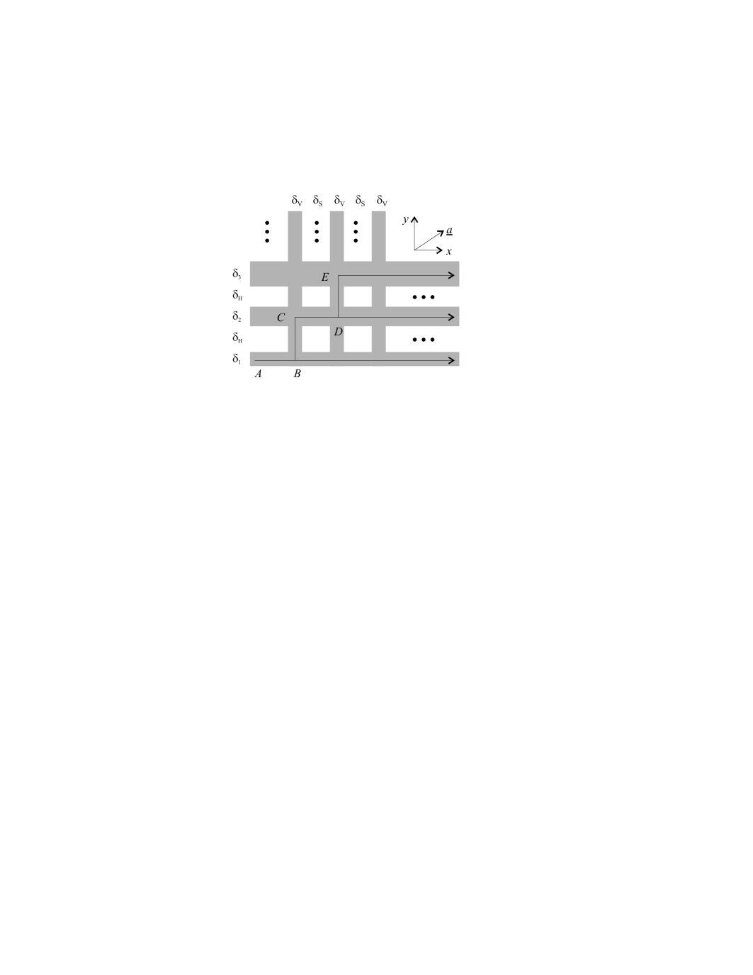
Figure 1:

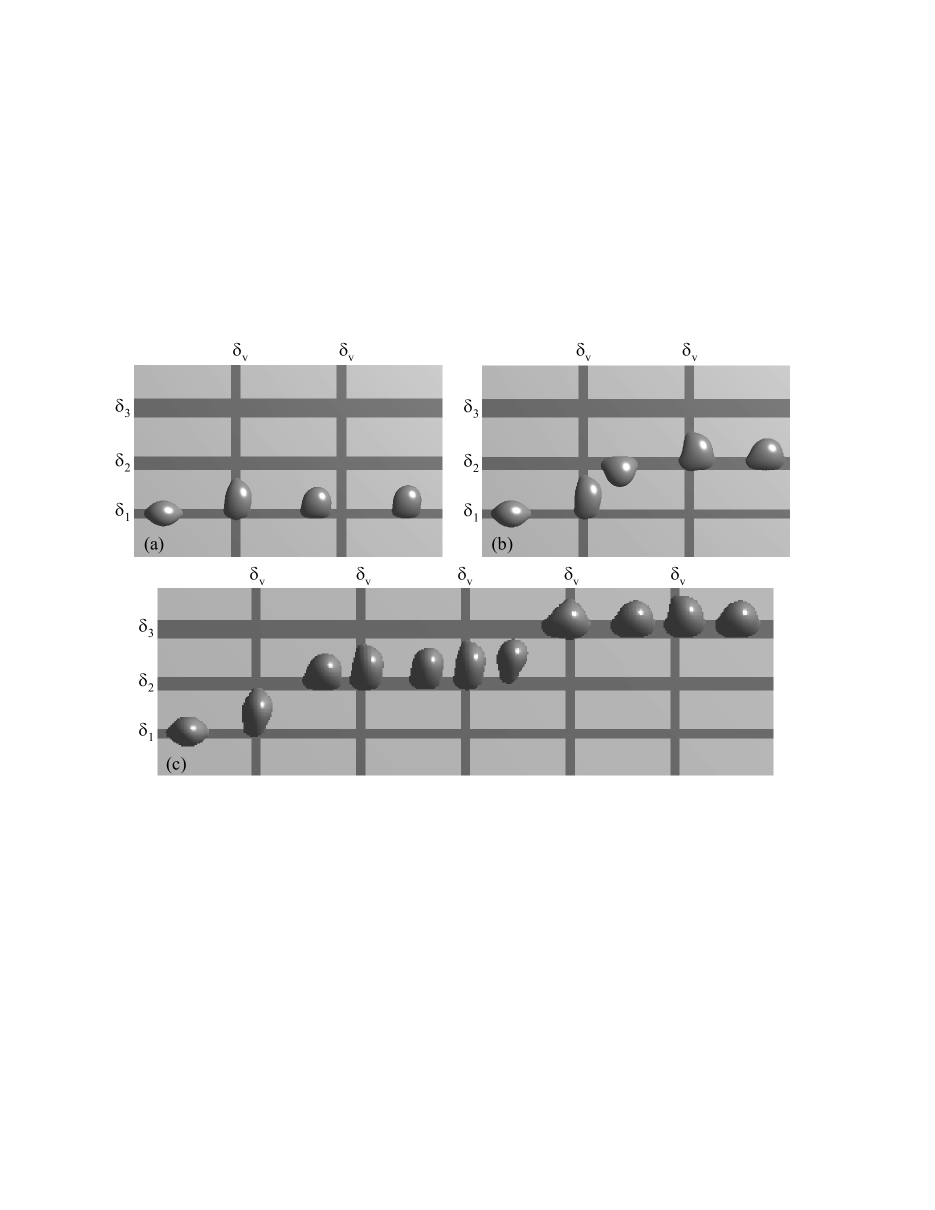
Figure 2:

.

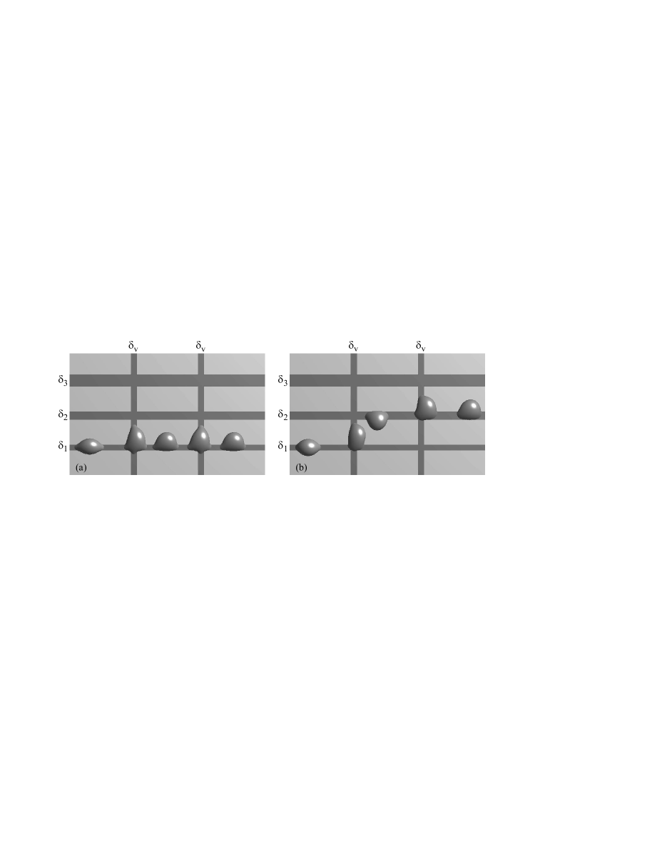
Figure 3:

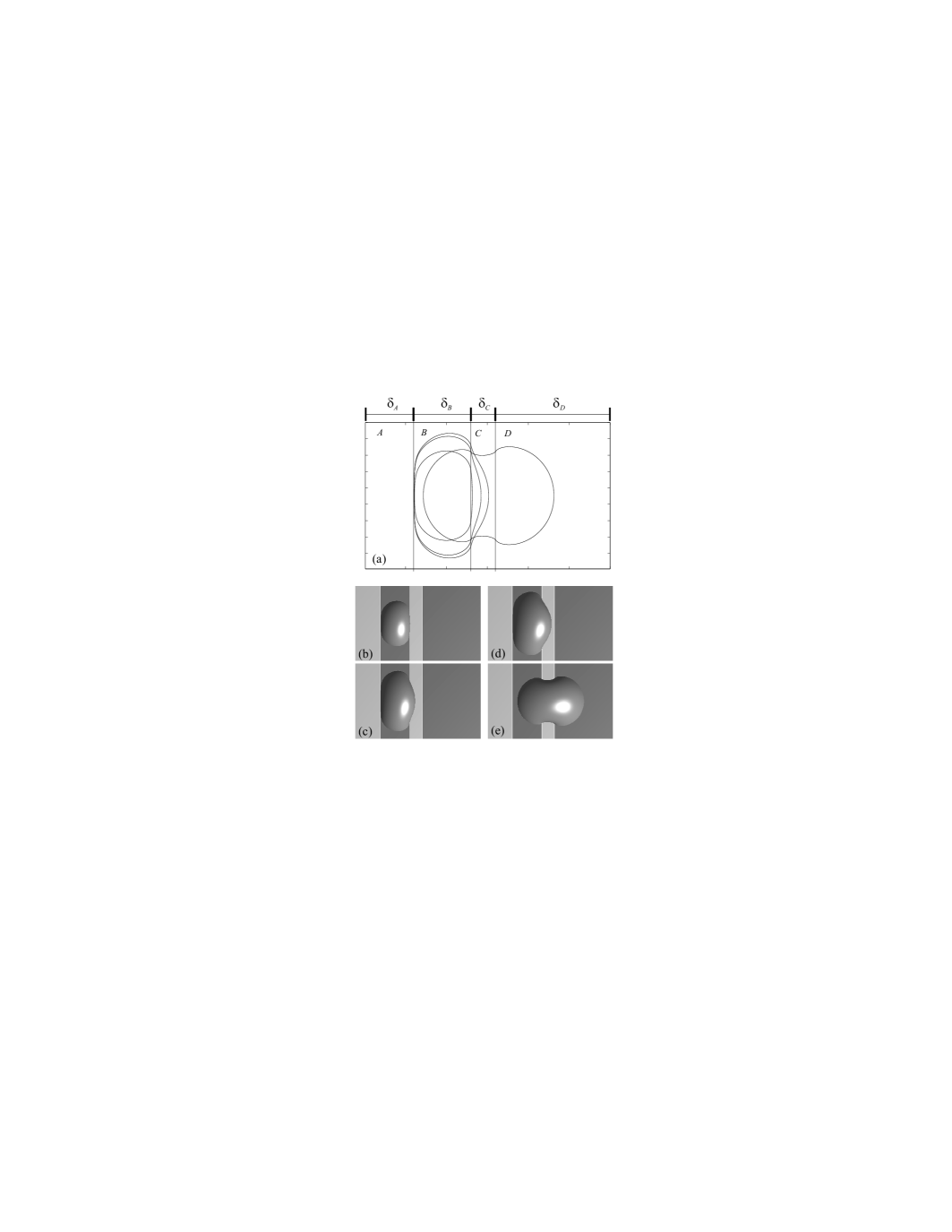
Figure 4:

.

References

- (1) Kusumaatmaja, H.; Léopoldès, J.; Dupuis A.; Yeomans, J. M. Europhys. Lett. 2006, 73, 740.
- (2) Léopoldès J.; Dupuis, A.; Yeomans, J. M. Langmuir 2003, 19, 9818.
- (3) Dupuis, A.; Yeomans, J. M. Fut. Gen. Comp. Sys. 2004, 20, 993.
- (4) Dupuis, A.; Léopoldès, J.; Bucknall, D. G.; Yeomans, J. M. Appl. Phys. Lett. 2005, 87, 024103.
- (5) Gau, G.; Hermingaus, H.; Lenz P.; Lipowsky, R. Science 1999, 283, 46.
- (6) Lenz P.; Lipowsky, R. Phys. Rev. Lett. 1998, 80, 1920.
- (7) Brinkmann, M.; Lipowsky, R. J. Appl. Phys. 2002, 92, 4296.
- (8) Darhuber, A. A.; Troian, S. M.; Miller, S. M.; Wagner, S. J. Appl. Phys. 2000, 87, 7768.
- (9) Darhuber, A. A.; Troian, S. M. Annu. Rev. Fluid Mech. 2005, 37, 425.
- (10) Mugele, F.; Klingner, A.; Buehrle, J.; Steinhauser, D.; Herminghaus, S. J. Phys.: Condens. Matter 2005, 17, S559.
- (11) Mugele, F.; Baret, J. C. J. Phys.:Condens. Matter 2005, 17, R705.
- (12) Blossey, R. Nature Materials 2003, 2, 301.
- (13) Parker, A. R.; Lawrence, C. R. Nature 2001, 414, 33.
- (14) Zhao, B.; Moore, J. S.; Beebe, D. J. Langmuir 2003, 19, 1873.
- (15) Zhao, B.; Moore, J. S.; Beebe, D. J. Science 2001, 291, 1023.
- (16) Handique, K.; Burke, D. T.; Mastrangelo, C. H.; Burns, M. A. Anal. Chem. 2000, 72, 4100.
- (17) Link, D. R.; Anna, S. L.; Weitz, D. A.; Stone, H. A. Phys. Rev. Lett. 2004, 92, 054503.
- (18) Squires, T. M.; Quake, S. Rev. Mod. Phys. 2005, 77, 977.
- (19) Kuksenok, O.; Jasnow, D.; Yeomans, J. M.; Balazs, A. C. Phys. Rev. Lett. 2003, 91, 108303.
- (20) Mo, G. C. H.; Kwok, D. Y. Appl. Phys. Lett. 88, 064103 (2006).
- (21) Dittrich, P. S.; Schwille, P. Annal. Chem. 2003, 75, 5767.
- (22) Fu, A. Y.; Chou, H-P; Spence, C.; Arnold, F. H.; Quake, S. R. Annal. Chem. 2002, 74, 2451.
- (23) Wang, M. M.; Tu, E.; Raymond, D. E.; Yang, J. M.; Zhang, H.; Hagen, N.; Dees, B.; Mercer, E. M.; Forster, A. H.; Kariv, I.; Marchand, P. J.; Butler, W. F. Nature Biotechnology 2005, 23, 83.
- (24) Ahn, K.; Kerbage, C.; Hunt, T. P.; Westervelt, R. M.; Link, D. R.; Weitz, D. A. Appl. Phys. Lett. 2006, 88, 024104.
- (25) Tan, Y. C.; Fisher, J. S.; Lee, A. I.; Cristini, V.; Lee, A. P. Lab Chip 2004, 4, 292.
- (26) Pollack, M. G.; Shenderov, A. D.; Fair, R. B. Lab Chip 2002, 2, 96.
- (27) Schwartz, J. A.; Vykoukal, J. V.; Gascoyne, P. R. C. Lab Chip 2004, 4, 11.
- (28) Sugiura, S.; Nakajima, M.; Iwamoto, S.; Seki, M. Langmuir 2001, 17, 5562.
- (29) Gañán-Calvo, A. M. Phys. Rev. Lett. 1998, 80, 285.
- (30) Anna, S. L.; Bontoux, N.; Stone, H. A. Appl. Phys. Lett. 2003, 82, 364.
- (31) Briant, A. J.; Wagner, A. J.; Yeomans, J. M. Phys. Rev. E 2004, 69, 031602.
- (32) Swift, M. R.; Orlandini, E.; Osborn, W. R.; Yeomans, J. M. Phys. Rev. E 1996, 54, 5041.
- (33) Succi, S. The Lattice Boltzmann Equation, For Fluid Dynamics and Beyond; Oxford University Press: 2001.
- (34) Cahn, J.W. J. Chem. Phys. 1977, 66, 3667.