Non-Markovian Lévy diffusion in nonhomogeneous media

Abstract

We study the diffusion equation with a position-dependent, power-law diffusion coefficient. The equation possesses the Riesz-Weyl fractional operator and includes a memory kernel. It is solved in the diffusion limit of small wave numbers. Two kernels are considered in detail: the exponential kernel, for which the problem resolves itself to the telegrapher’s equation, and the power-law one. The resulting distributions have the form of the Lévy process for any kernel. The renormalized fractional moment is introduced to compare different cases with respect to the diffusion properties of the system.

I Introduction

Diffusion processes are usually described in terms of either differential or fractional equations which contain a constant diffusion coefficient. In many physical problems, however, that coefficient depends on the position variable and such dependence is important lop . As a typical example can serve the transport in porous, inhomogeneous media and in plasmas. Modelling the aggregation of interacting particles must take into account nonlocal effects, since the particle mobility depends on the average density hol : the coalescence of particles results from long-range interactions (the Poisson-Smoluchowski paradigm) and the corresponding evolution equations contain a position-dependent coefficient. That modelling can be accomplished directly, via the non-local Fokker-Planck equation, in which the term with the space derivative is multiplied by a kernel and integrated over the position mal . A similar method, applicable to the Lévy processes, consists in the integrating over the Lévy index, with some kernel (the distributed order space fractional equation) che . The spatial inhomogeneity can be also taken into account as an external potential which may substantially change the diffusive properties of the stochastic system, in particular of the Lévy flights bro .

The Lévy distributions constitute the most general class of stable processes and the Gaussian distribution is their special case. One can expect that the Lévy (and non-Gaussian) distributions emerge in transport processes for which the observable values experience long jumps, e.g. due to the existence of long range correlations. The theory of the Lévy flights is applicable to problems from various branches of science and technology. Moreover, the handling of specific and realistic systems often requires taking into account both memory effects and inhomogeneity of the media. As a typical example of the nonhomogeneous problem can serve the diffusion in the porous media; they often display the fractal structure and the diffusion on the macro- and mesoscale can be expressed by a stochastic equation driven by the Lévy process par . In general, the transport in fractal media can be described by the fractional Fokker-Planck equation with a variable, position dependent, diffusion coefficient met3 ; met4 ; tar . The Lévy flights bring about the accelerated diffusion in the reaction-diffusion systems cas and the probability distribution for that process is expressed by the fractional Fisher-Kolmogorov equation. The Lévy processes are typical for problems of high complexity, in particular in biological systems wes where the fractal structures are also encountered. For example, the lipid diffusion in biomembranes has the characteristics of the Lévy process but it can no longer be regarded as Markovian. The theory of Nonnenmacher non takes into account the memory effects, as well as the fractal structure of the medium; the diffusion coefficient depends on the variable diameter of the holes in the solvent through which the molecules jump. The application of the Lévy processes is natural also in many social and environmental problems. Recently, it has been established bro1 that the people mobility, estimated by the bank notes circulation and studied in terms of the stochastic fractional equations, strongly depends on geographical and sociological conditions. Therefore, its study requires including position-dependent quantities. That problem is directly related to the spread of infectious diseases. It has been demonstrated in the example of the SARS epidemic and by means of percolation model simulations fuji that the disease can spread very rapidly. Usually one assumes that the infection probability at a given distance is Lévy distributed due to the long-range interactions but the process is local in time mol . On the other hand, the percolation model of the epidemics developed in Ref.jim is restricted to short-range interactions (is local in space) but it introduces the incubation times which obey the Lévy statistics and then the model is non-Markovian.

In Refs.kam1 ; sro1 , the master equation for a jumping process, stationary and Markovian, has been studied. That process is a version of the coupled continuous time random walk (CTRW), defined in terms of two probability distributions: the Poissonian waiting time distribution with the position-dependent jumping frequency and a jump-size distribution. The standard technique to handle such master equations is the Kramers-Moyal expansion which produces the Fokker-Planck equation for the Gaussian jumping size distribution and it yields correct results for large times and large distances uwa1 . For the Lévy distributed jumping size, the Fokker-Planck equation becomes the fractional diffusion equation, with the Riesz-Weyl fractional operator and the variable coefficient $D(x)$. Formally, it can be derived from the master equation by taking the Fourier transform and by neglecting the higher terms in the wave number expansion of the jumping-size distribution (the diffusion approximation) sro . The equation reads

$$\frac{\partial p(x,t)}{\partial t}=K^{\mu}\frac{\partial^{\mu}[D(x)p(x,t)]}{\partial|x|^{\mu}},$$ (1)

where $1<\mu<2$. Since the diffusion coefficient is just the jumping frequency, the medium inhomogeneity enters the problem via the $x$-dependent waiting time distribution. For the Gaussian case ($\mu=2$), all kinds of diffusion, both normal and anomalous, are predicted sro and they are determined by the jumping frequency.

The Eq.(1) can be regarded as a special case of a more general problem than the random walk and which traces back to the microscopic foundations of the nonequilibrium statistical mechanics. The well-known achievement of Zwanzig zwa was the derivation of the non-Markovian kinetic equation for the probability distribution in the space of macroscopic state variables. More precisely, by starting from the Liouville-von Neumann equation for the density operator $\rho$: $i\hbar\partial\rho/\partial t=[H,\rho]$, where $H$ is the Hamiltonian of the system, one can obtain the generalized master equation:

$$\frac{\partial P_{\xi}(t)}{\partial t}=\int_{0}^{t}dt^{\prime}\phi(t-t^{\prime})\sum_{\mu}[F_{\xi\mu}P_{\mu}(t^{\prime})-F_{\mu\xi}P_{\xi}(t^{\prime})],$$ (2)

where $P_{\xi}$ denotes the diagonal elements of the density matrix and $F_{\mu\xi}$ are the transition rates ken . Then the equation is non-Markovian and it contains the memory kernel $\phi(t)$. Markovian equations like (1) follow from the generalized master equation if the memory effects are negligible. However, usually this is not the case. We have already discussed the examples of the Lévy processes, with power-law tails of the distribution, which exhibit memory effects. In fact, the importance of these effects was realized a long time ago, e.g. in the description of the resonance transfer of the excitation energy between molecules ken . The detailed calculation for the anthracene molecules shows that the memory kernel is exponential and the generalized, nonlocal in time, master equation must be applied to get proper results for small times. One can expect that memory effects are still more pronounced for systems with the characteristic decay rate slower than exponential, that often happens for atomic and molecular systems bud . Stochastic dynamical processes are generally nonlocal in time due to the finite time of the interaction with the environment. Moreover, for a stochastic system which is coupled to a fractal heat bath via a random matrix interaction lut , the finite correlations emerge and its relaxation has to be described in terms of the generalized, non-Markovian Langevin equation, with the memory friction term kubo ; luc . Also the speed of transport is affected by the memory. In the non-Markovian CTRW processes it hampers the dynamics and such systems are subdiffusive met . Such processes are described by the generalized master equation, with a memory kernel, if the waiting time distribution possesses long, algebraic tails. That equation follows directly from the generalized Chapman-Kolmogorov equation which determines the probability distribution in the phase space metk ; metz .

By applying the nearest-neighbour approximation on the transition rates $F_{\mu\xi}$ and taking the continuum limit ken , one obtains from the Eq.(2) the non-Markovian Fokker-Planck equation. In the presence of long-range correlations, however, the nearest-neighbour approximation is no longer valid. If the transition rates are symmetric and distributed according to the Lévy statistics in the continuum limit, the Kramers-Moyal expansion produces the fractional derivative, instead of the Gaussian. Then, for the variable diffusion coefficient $D(x)$, the equation which corresponds to the Eq.(2) becomes

$$\frac{\partial p_{\gamma}(x,t)}{\partial t}=\int_{0}^{t}K_{\gamma}(t-t^{\prime}){\mathcal{L}}_{x}[p_{\gamma}(x,t^{\prime})]dt^{\prime},$$ (3)

where the operator

$${\mathcal{L}}_{x}=K^{\mu}\frac{\partial^{\mu}}{\partial|x|^{\mu}}D(x)$$ (4)

acts only on the $x$ variable. The parameter $\gamma$ measures the rate of the memory loss.

The Eq.(3) is of interest both from quantum and classical point of view. In the atomic and molecular physics e.g. in a few-modes spin boson model won and the random-matrix theory won1 , where the decay rate is slow, an equation analogous to the Eq.(3) can be applied. The operator ${\mathcal{L}}_{x}$ is then expressed in terms of the ”superoperator” which represents an instantaneous intervention of the environment over the system bud and it can assume a quite general form. In the classical context, the Eq.(3) has been discussed in Ref.sok ; the operator ${\mathcal{L}}_{x}$ has the Fokker-Planck form in this case, with the constant diffusion coefficient and a potential force.

In this paper we study the diffusion problem for systems which are driven by the Lévy distributed transition rate and for which both the medium inhomogeneity and the memory effects are important. We assume $D(x)=|x|^{-\theta}$ $(\theta>-1)$. The power-law form of the diffusion coefficient has been used to describe some physical phenomena, e.g. the transport of fast electrons in a hot plasma ved and the turbulent two-particle diffusion fuj . It is also used in theoretical analyses of the fractional Fokker-Planck equation len ; len1 ; kwo1 ; ass , e.g. as an ansatz for the problem of diffusion in the fractal media osh ; met3 ; met4 ; tar . Obviously, for the Markovian case $K_{\gamma}(t)=\delta(t)$, the Eq.(3) resolves itself to the Eq.(1).

In Sec.II we solve the fractional telegrapher’s equation which follows from the Eq.(3) for the case of the exponential memory kernel $K_{\gamma}(t)$. The solution for an arbitrary kernel, expressed in the form of the Laplace transform, is derived in Sec.III. Moreover, the case of the power-law kernel is solved in details. In Sec.IV we derive the fractional moments and discuss their application to the description of the diffusion process. The results presented in the paper are summarized in Sec.V.

II The exponential kernel

If the memory effects are weak, we can assume that the kernel $K_{\gamma}(t)$ decays exponentially. Then let us consider the following kernel:

$$K_{\gamma}(t)=\gamma e^{-\gamma t}~{}~{}~{}~{}~{}~{}~{}(\gamma>0)$$ (5)

which becomes the delta function in the limit $\gamma\to\infty$ (the Markovian case). In this case, the integral equation, Eq.(3), reduces itself to a differential equation. It can be derived by inserting the Eq.(5) to the Eq.(3) and by differentiating twice over time, in order to get rid of the integral. Finally, we get the following equation

$$\frac{\partial^{2}p_{\gamma}(x,t)}{\partial t^{2}}+\gamma\frac{\partial p_{\gamma}(x,t)}{\partial t}=K^{\mu}\gamma\frac{\partial^{\mu}[|x|^{-\theta}p_{\gamma}(x,t)]}{\partial|x|^{\mu}},$$ (6)

which is a generalized and fractional version of the well-known telegrapher’s equation. Originaly, the telegrapher’s equation, which is the hyperbolic one, has been introduced into the theory of the stochastic processes by Cattaneo catt in order to avoid infinitely fast propagation for very small times. Its fractional generalization describes e.g. a two-state process with the correlated noise metn and it predicts the inhanced diffusion in the limit of long time. On the other hand, in the case of the divergent second moment, the telegrapher’s equation with the Riesz-Weyl derivative results from the fractional Klein-Kramers equation for the Lévy distributed jumping size metz . In that equation, the parameter $\gamma$ has a sense of the damping constant in the corresponding Langevin equation.

In the diffusion limit of small wave numbers, the Markovian equation, Eq.(1), is satisfied by the Fox function $H_{2,2}^{1,1}$ sro . Since our main objective is to study the diffusion problem, we restrict also the present analysis to that limit. We will try to find the solution of the Eq.(6) in the same form as for the Markovian equation. Therefore we assume:

$$p_{\gamma}(x,t)=NaH_{2,2}^{1,1}\left[a|x|\left|\begin{array}[]{c}(a_{1},A_{1}),(a_{2},A_{2})\\ \\ (b_{1},B_{1}),(b_{2},B_{2})\end{array}\right.\right],$$ (10)

where the time dependence is restricted to the function $a(t)$ and $N$ is the normalization constant. The method of solution, described in Ref.sro , consists in the inserting of the Fourier transform of the expression (10) into the Fourier transformed Eq.(6). Then we determine the coefficients of the Fox function by demanding that the Eq.(6) should be satisfied in the diffusion limit, i.e. for small wave numbers. In fact, the latest assumption does not introduce any additional idealization since the equation itself is valid only in the diffusion limit.

We start with the Fourier transform of the Eq.(6); it reads

$$\frac{\partial^{2}{\widetilde{p}}_{\gamma}(k,t)}{\partial t^{2}}+\gamma\frac{\partial{\widetilde{p}}_{\gamma}(k,t)}{\partial t}=-K^{\mu}\gamma|k|^{\mu}{\mathcal{F}}[|x|^{-\theta}p_{\gamma}(x,t)].$$ (11)

The Fourier transform of the Fox function can be expressed also in terms of the Fox function (for the definition and some useful properties of the Fox functions see Ref.sro and references therein). Due to the multiplication rule, the product $|x|^{-\theta}p_{\gamma}(x,t)$ is the Fox function as well. Both sides of the Eq.(11) can now be expanded in series of fractional powers of $|k|$. We can satisfy the Eq.(11) by a suitable choice of the parameters of the function (10) and by neglecting the terms higher than $|k|^{\mu}$. The results are the following. The expansion of the functions on the lhs and rhs, respectively, reads: ${\widetilde{p}_{\gamma}}(k,t)\approx 1-Nh_{\mu}a^{-\mu}|k|^{\mu}$ and ${\mathcal{F}}[|x|^{-\theta}p_{\gamma}(x,t)]\approx Nh_{0}^{(\theta)}a^{\theta}$, with the following coefficients: $h_{0}^{(\theta)}=2(\mu+\theta)/(2+\theta)$ and $h_{\mu}=-2\frac{(\mu+\theta)^{2}}{\pi}\Gamma(-\mu)\Gamma(\mu+\theta)\cos(\mu\pi/2)\sin(\frac{\mu+\theta}{2+\theta}\pi)$. The vanishing of all other terms of the order less than $\mu$ is the necessary condition to satisfy the Eq.(11). The solution takes the form

$$p_{\gamma}(x,t)=NaH_{2,2}^{1,1}\left[a|x|\left|\begin{array}[]{l}(1-\frac{1-\theta}{\mu+\theta},\frac{1}{\mu+\theta}),(1-\frac{1-\theta}{2+\theta},\frac{1}{2+\theta})\\ \\ (\theta,1),(1-\frac{1-\theta}{2+\theta},\frac{1}{2+\theta})\end{array}\right.\right]$$ (15)

and the coefficients $b_{1}$ and $B_{1}$ are responsible for the distribution behaviour near $x=0$. $b_{1}$ and $B_{1}$ cannot be determined in the diffusive limit and they are meaningless from the point of view of the diffusion process; the values $\theta$ and $1$ we have assumed correspond to the jumping process, considered in Ref.sro . Generally, the Eq.(3) is satisfied by the function (15) for any choice of the coefficients $b_{1}$ and $B_{1}>0$, such that $b_{1}\to 0$ and $B_{1}\to 1$ for $\theta\to 0$. The normalization factor $N$ can be determined in a simple way from the formula $N=[2\chi(-1)]^{-1}$, where $\chi(-s)$ is the Mellin transform of the Fox function. A simple algebra yields

$$N=-\frac{\pi}{2}\left[\Gamma(1+\theta)\Gamma\left(-\frac{\theta}{\mu+\theta}\right)\sin\left(\frac{\theta}{2+\theta}\pi\right)\right]^{-1}.$$ (16)

Alternatively, since $|k|$ is small, we can express the Fourier transform of the solution as

$${\widetilde{p}_{\gamma}}(k,t)\approx 1-\sigma^{\mu}|k|^{\mu}\approx\exp(-\sigma^{\mu}|k|^{\mu}),$$ (17)

where

$$\sigma^{\mu}=K^{-\mu}\frac{(\mu+\theta)^{2}\Gamma(-\mu)\Gamma(\mu+\theta)\cos(\mu\pi/2)\sin(\frac{\mu+\theta}{2+\theta})}{\Gamma(1+\theta)\Gamma(-\frac{\theta}{\mu+\theta})\sin(\frac{\theta}{2+\theta}\pi)}\,a^{-\mu}.$$ (18)

The Eq.(17) means that the solution of Eq.(3) coincides with the Lévy process in the limit $k\to 0$. Then the solution (15) can be expressed in the form which is generic for any symmetric Lévy distribution sch :

$$p_{\gamma}(x,t)=\frac{1}{\mu\sigma}H_{2,2}^{1,1}\left[\frac{|x|}{\sigma}\left|\begin{array}[]{l}(1-1/\mu,1/\mu),(1/2,1/2)\\ \\ (0,1),(1/2,1/2)\end{array}\right.\right].$$ (22)

The formula (18) establishes the relation between the solutions (15) and (22). Those expressions are equivalent only in the limit $k\to 0$ and they behave differently for small $|x|$. We will demonstrate in Sec.III that the Lévy process is the solution of the Eq.(3) for any kernel. Therefore, the form (22) is quite universal and we apply it in the following. The problem is reduced in this way to evaluating the function $\sigma(t)$.

Now, the Eq.(11) becomes the ordinary differential equation:

$$\frac{1}{\gamma}\ddot{\xi}=-\dot{\xi}+K^{\mu}\frac{h_{0}^{(\theta)}}{h_{\mu}}\xi^{-\theta/\mu},$$ (23)

where $\xi(t)=a^{-\mu}$. We assume the following initial conditions: $\xi(0)=\dot{\xi}(0)=0$ which correspond to the condition $p_{\gamma}(x,0)=\delta(x)$. The Eq.(23) has the structure of the equation of motion with a ”friction term”, a positive ”driving force”, and a ”mass” $1/\gamma$. The meaning of the quantity $\xi$, the time evolution of which the Eq.(23) describes, remains to be determined. The variable $\xi$, as well as $\dot{\xi}$, rises with time and finally the balance of ”forces”, given by the equation

$$\dot{\xi}-K^{\mu}\frac{h_{0}^{(\theta)}}{h_{\mu}}\xi^{-\theta/\mu}=0,$$ (24)

is reached. Note that the above expression is equivalent to the Eq.(23) in the Markovian limit $\gamma\to\infty$. Therefore $p_{\gamma}(x,t)=p_{\infty}(x,t)=p(x,t)$ for $t\to\infty$. The solution of the Eq.(24) produces the result

$$a(t)=\left[K^{\mu}\frac{h_{0}^{(\theta)}}{h_{\mu}}\left(1+\frac{\theta}{\mu}\right)t\right]^{-1/(\mu+\theta)}~{}~{}~{}~{}~{}~{}~{}(t\to\infty)$$ (25)

which corresponds to the exact solution (for arbitrary time) for the Markovian limit, $p(x,t)$.

The case of the constant diffusion coefficient, $\theta=0$, is a particular case and it can be solved easily. The solution of the Eq.(23) leads to the following result

$$a(t)=\frac{1}{K}\left[-\frac{1}{\gamma}(1-e^{-\gamma t})+t\right]^{-1/\mu}.$$ (26)

For $\theta\neq 0$ and arbitrary time, the Eq.(23) can be solved by the numerical integration and the distribution $p_{\gamma}(x,t)$ determined from the Eq.(22). To evaluate the Fox function we use the general formula for its series expansion and then the Eq.(22) can be expressed in the computable form:

$$p_{\gamma}(x,t)=\frac{1}{\pi\sigma\mu}\sum_{n=0}^{\infty}\frac{\Gamma[1+(2n+1)/\mu]}{(2n+1)!!}(-1)^{n}\left(\frac{x}{\sigma}\right)^{2n}.$$ (27)

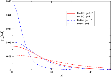
Figure 1: (Color online) Probability distributions for the case of the exponential kernel with $\mu=1.5$, calculated from the Eqs.(23), (18), and (27), for $t=50$. The initial condition is $p_{\gamma}(x,0)=\delta(x)$.

Fig.1 presents some exemplary probability distributions, so chosen to illustrate the influence of the memory on the time evolution. Since the series (27) is poorly convergent, the evaluating of the distribution for large $|x|$ required the quadruple computer precision uwa . The case with $\gamma=3$ is close to the Markovian one; a comparison with the case characterized by the long memory shows that the spread of the distribution slows down with the decreasing value of $\gamma$, i.e. for stronger memory (larger ”inertia” in the Eq.(23)). In the limit $t\to\infty$ the curves which correspond to different $\gamma$ values and the same $\theta$ – coincide.

III The general case

The description by means of the Eq.(3) with the exponential memory kernel does not apply to systems with long-time correlations and small decay rate. In the study of realistic systems one encounters a variety of forms of the kernel; some of them are very complex. It is typical for natural signals that they do not represent a simple kinetics, characterised by a unique Hurst exponent. Random processes which take into account the whole spectrum of the time-dependent Hurst exponents serve then as useful models. This concept, applied to the fractional equations formalism, leads to the integration over the order of differentiation (the distributed-order diffusion equation) che and the kernel assumes the integral form: $\int f(\alpha)t^{-\alpha}d\alpha$. Reactions in polymer systems are also described by using complicated kernels cher ; ban . Therefore, in this Section we consider the Eq.(3) for the case as general as possible. We will demonstrate that the solution in a closed form can be obtained for the arbitrary kernel.

The Eq.(3) has the structure of the Volterra integro-differential equation with the kernel which depends on the difference of its arguments. Therefore, methods using Laplace transforms are applicable. Following Sokolov sok , we apply a method of the integral decomposition which allows us to express the required solution by the solution of the corresponding Markovian equation (1). Let us define the function $T(\tau,t)$ by its Laplace transform:

$$T^{\star}(\tau,u)=\frac{1}{K_{\gamma}^{\star}}\exp\left(-\tau\frac{u}{K_{\gamma}^{\star}}\right).$$ (28)

If we know the function $T(\tau,t)$, the probability distribution $p_{\gamma}(x,t)$ can be obtained by a simple integration:

$$p_{\gamma}(x,t)=\int_{0}^{\infty}p(x,\tau)T(\tau,t)d\tau.$$ (29)

However, since the inversion of the Eq.(28) is difficult for any kernel, it is expedient to get rid of $T$. To achieve that, we take the Fourier transform from the Eq.(29) and eliminate the function $T(\tau,t)$ by using the definition (28). The final solution is of the form of the following Fourier-Laplace transform

$${\widetilde{p}}_{\gamma}^{\star}(k,u)=\frac{1}{K_{\gamma}^{\star}}{\widetilde{p}}^{\star}\left(k,\frac{u}{K_{\gamma}^{\star}}\right).$$ (30)

The above formalism can be applied for any kernel $K_{\gamma}$ and any operator ${\mathcal{L}}_{x}$; the main difficulty consists in inversion of the Laplace transforms.

First of all, we find that if the Markovian process $p(x,t)$ is Lévy distributed in the diffusion limit $k\to 0$, then the non-Markovian process is also the Lévy process in this limit. Indeed, the Fourier transform of the Markovian solution is given by the Eq.(17), where $\sigma(t)$ follows from the Eqs.(18) and (25). Then we take the Laplace transform from that expression and insert the result to the Eq.(30): ${\widetilde{p}}_{\gamma}^{\star}(k,u)=1/u-F^{\star}(u)|k|^{\mu}$. Finally, the inversion of the Laplace transform yields

$${\widetilde{p}}_{\gamma}(k,t)=1-F(t)|k|^{\mu},$$ (31)

which is just the Fourier representation of the Lévy distribution for small $|k|$. To get the function $F(t)$ we need to invert the Laplace transform

$$F^{\star}(u)=\frac{Nh_{\mu}}{K_{\gamma}^{\star}(u)}[a^{-\mu}]^{\star}(u/K_{\gamma}^{\star})$$ (32)

and we assume that this inverse transform exists. The solution is given by the Eq.(22), where $\sigma(t)=[F(t)]^{1/\mu}$.

We will consider two particular cases in detail. In the case of the exponential memory kernel (5), discussed already in Sec.II, we have $K_{\gamma}^{\star}(u)=\gamma/(u+\gamma)$ and the Eq.(30) produces the following result

$${\widetilde{p}}_{\gamma}^{\star}(k,u)=\frac{1}{u}-a_{0}\Gamma(1+\alpha)\gamma^{\alpha}|k|^{\mu}u^{-(\alpha+1)}(u+\gamma)^{-\alpha},$$ (33)

where $a_{0}=Nh_{\mu}^{1-\alpha}(K^{\mu}h_{0}^{(\theta)}\alpha/\mu)^{\alpha}$ and $\alpha=\mu/(\mu+\theta)$. The above expression cannot be inverted in closed form. However, if we are interested only in large times, the last term in the Eq.(33) can be expanded around $u=0$: $(u+\gamma)^{-\alpha}\approx\gamma^{-\alpha}-\alpha\gamma^{-(\alpha+1)}u$. Then the inversion of the Laplace transform yields

$${\widetilde{p}}_{\gamma}(k,t)=1-a_{0}|k|^{\mu}\left(t^{\alpha}-\frac{\alpha^{2}}{\gamma}t^{\alpha-1}\right)~{}~{}~{}~{}~{}~{}~{}(t\to\infty)$$ (34)

and this expression demonstrates how the solution $p_{\gamma}$ approaches its asymptotic, Markovian form. The final solution, valid for large $t$, is given by the Eq.(22) with $\sigma=[a_{0}(t^{\alpha}-\frac{\alpha^{2}}{\gamma}t^{\alpha-1})]^{1/\mu}$.

The other physically important kernel has the power-law form, with long tails:

$$K_{\gamma}(t)=\frac{t^{-\gamma}}{\Gamma(1-\gamma)}~{}~{}~{}~{}~{}(0<\gamma<1).$$ (35)

The equation (3) with the kernel (35) is usually presented as the fractional equation with the Riemann-Liouville derivative old – which is equivalent to the Caputo operator for a special choice of the initial conditions – in the following form

$$\frac{\partial p_{\gamma}(x,t)}{\partial t}={{}_{0}}D_{t}^{\gamma-1}{\mathcal{L}}_{x}[p_{\gamma}(x,t)].$$ (36)

The power-law kernels are used to describe subdiffusive relaxation e.g. in the framework of the CTRW met . They emerge also as a result of the coupling to the fractal heat bath via the random matrix interaction lut . To solve the Eq.(3) we follow the same procedure as for the exponential kernel. The Laplace transform of the Eq.(35) reads $K_{\gamma}^{\star}(u)=u^{\gamma-1}$ and the Eq.(30) takes the form

$${\widetilde{p}}_{\gamma}^{\star}(k,u)=\frac{1}{u}-a_{0}\Gamma(1+\alpha)\gamma^{\alpha}|k|^{\mu}u^{-2\alpha+\gamma\alpha-1}.$$ (37)

The inversion can be easily performed:

$${\widetilde{p}}_{\gamma}(k,t)=1-\frac{a_{0}\gamma^{\alpha}\Gamma(1+\alpha)}{\Gamma(2\alpha-\gamma\alpha+1)}|k|^{\mu}t^{2\alpha-\gamma\alpha}\equiv 1-F(t)|k|^{\mu}.$$ (38)

Clearly, the above solution does not converge with time to the Markovian asymptotics, $F(t)\sim t^{\alpha}$, in contrast to the case of the exponential kernel.

To conclude this Section, we want to mention yet another approach to the Eq.(3), which is a direct generalization of the method applied for the telegrapher’s equation in Sec.II. Inserting the expansion of the functions ${\widetilde{p}_{\gamma}}(k,t)$ and ${\mathcal{F}}[|x|^{-\theta}p_{\gamma}(x,t)]$ to the Eq.(3) confirms the finding that the solution can be expressed in terms of the Fox function $H_{2,2}^{1,1}$ and it is Lévy distributed. The resulting equation is a generalization of the Eq.(23) and it determines the function $\sigma(t)$:

$$\frac{d\xi}{dt}=K^{\mu}\frac{h_{0}^{(\theta)}}{h_{\mu}}\int_{0}^{t}K_{\gamma}(t-t^{\prime})\xi^{-\theta/\mu}dt^{\prime}.$$ (39)

Mathematically, the Eq.(39) has the form of the nonlinear Volterra integro-differential equation. Since the numerical inversion of the Laplace transforms is not always an easy task (methods are often unstable), the numerical solving of the Eq.(39) could be a useful alternative to the Eq.(31).

IV Diffusion

The diffusion process is usually characterized by the time dependence of the second moment of the probability distribution: if this dependence is linear in the limit of long time, the diffusion is called normal. There are many examples of physical systems for which the variance rises faster than linearly with time (hyperdiffusion), or slower (subdiffusion). Such behaviours are typical for transport in the disordered media bou and systems with traps and barriers. In the realm of dynamical systems, a substantial acceleration of the diffusion is caused by the presence of regular structures in the phase space zas . On the other hand, the subdiffusion appears in the non-Markovian version of CTRW, as a result of a non-Poissonian, power-law form of the waiting time distribution met .

When we enter the field of the Lévy processes, the situation becomes more complicated. The stochastic variable performs very long jumps and their size is limited only by the size of whole system. As a result, the second moment, as well as all moments of the order $\mu$ or higher, is divergent. Mathematically, that follows from the fact that the tail of the Lévy distribution is the power-law: $\sim|x|^{-(1+\mu)}$. Therefore, one cannot describe the diffusion process in terms of the position variance and some other quantity which could serve as an estimation of the speed of transport is needed. One possibility is to consider still the second moment but with the integration limits restricted to a time-dependent interval (the walker in the imaginary growing box) jes . On the other hand, one can derive the fractional moments of the order $\delta<\mu$.

By the derivation of the moments of the probability distribution $p_{\gamma}(x,t)$, Eq.(22), we utilize simple properties of the Mellin transform from the Fox function:

$$\langle|x|^{\delta}\rangle=2\int_{0}^{\infty}x^{\delta}p_{\gamma}(x,t)dx=\frac{2}{\mu}\sigma^{\delta}\chi(-\delta-1)=\frac{2}{\pi}\sigma^{\delta}\Gamma(\delta)\Gamma(1-\frac{\delta}{\mu})\sin(\delta\pi/2).$$ (40)

Let us consider two quantities: the renormalized moment of order $\mu$, defined by the following expression

$${\mathcal{M}}^{\mu}=\lim_{\epsilon\to 0^{+}}\epsilon\langle|x|^{\mu-\epsilon}\rangle=\frac{2}{\pi}\sigma^{\mu}\Gamma(\mu)\sin(\mu\pi/2),$$ (41)

where we applied the property: $\Gamma(x)\to 1/x$ for $x\to 0$, and then the fractional diffusion coefficient ${\mathcal{D}}^{(\mu)}(t)=\frac{1}{\Gamma(1+\mu)}\frac{1}{t}{\mathcal{M}}^{\mu}$. In the Markovian case, defined by the Eq.(1), the coefficient ${\mathcal{D}}^{(\mu)}$ is useful to classify the diffusion: for $\theta<0$ it rises with time, for $\theta>0$ it falls, and it converges to a constant for $\theta=0$ sro . That pattern is consistent with the diffusion properties, defined in the ordinary sense, of the Fokker-Planck equation $(\mu=2)$. Therefore, in the following we will name all kinds of the diffusion – the subdiffusion, the normal diffusion, and the superdiffusion – according to the time dependence of the coefficient ${\mathcal{D}}^{(\mu)}$.

We begin with the case of the exponential kernel. First we realize that, since $\sigma^{\mu}=Nh_{\mu}\xi$, the renormalized moment ${\mathcal{M}}^{\mu}$ is directly related to the variable $\xi$: ${\mathcal{M}}^{\mu}=\frac{2}{\pi}Nh_{\mu}\Gamma(\mu)\sin(\mu\pi/2)\xi$. Therefore, the interpretation of the Eq.(23) is straightforward: it describes the deterministic time evolution of the moment ${\mathcal{M}}^{\mu}$. The diffusion properties of the system remain unchanged, compared to the Markovian case, because in the limit $t\to\infty$ both solutions coincide. However, at small time the influence of the memory, which hampers both the spread of the distribution and the relaxation to the Markovian asymptotics, is visible. Fig.2 illustrates that effect for three values of $\theta$ which have different sign. The asymptotic, Markovian limit is achieved first for the subdiffusive case $\theta=0.4$.

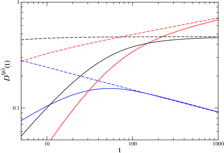
Figure 2: (Color online) The fractional diffusion coefficient for the case of the exponential kernel with $\gamma=0.05$ (solid lines) and $\gamma=3$ (dashed lines), as a function of time, obtained from numerical solving of the Eq.(23). Results for three values of $\theta$ are presented: $\theta=-0.2$ (upper lines for large $t$), $\theta=0$ (middle lines), and $\theta=0.4$ (lower lines); $\mu=1.5$.

For the case of the power law kernel we calculate the fractional diffusion coefficient by means of the Eq.(41); the quantity $\sigma^{\mu}(t)=F(t)$ is given by the Eq.(38). We obtain

$${\mathcal{D}}^{(\mu)}(t)=\frac{2a_{0}\gamma^{\alpha}\Gamma(1+\alpha)}{\pi\mu\Gamma(\alpha-\gamma\alpha+1)}\sin(\mu\pi/2)t^{2\alpha-\gamma\alpha-1}\sim t^{[\mu(1-\gamma)-\theta]/(\mu+\theta)}.$$ (42)

The diffusion properties of the system follow directly from the above formula. The influence of the parameter $\theta$, which quantifies the structure of the medium, is similar as in Markovian case sro : the larger is $\theta$ the weaker is diffusion. For $\theta\leq 0$, there is clearly the superdiffusion. For the positive $\theta$, the diffusion becomes weaker with $\theta$ and finally it turns to the subdiffusion; the critical value, which corresponds to the normal diffusion, is $\theta_{cr}=\mu(1-\gamma)$. On the other hand, if $0<\theta<\mu$, there is a critical value of $\gamma$ which separates the superdiffusion from the subdiffusion: $\gamma_{cr}=1-\theta/\mu$. For $\theta>\mu$ the motion is always subdiffusive. The parameter $\gamma$ measures the degree of the time nonlocality; it is the largest if $\gamma$ approaches 0. The diffusion speed grows if $\gamma$ diminishes because the system behaviour at large times becomes sensitive to the initial stages of the evolution when the distribution spreads rapidly. The latter conclusion shows that the memory can influence the diffusion in many ways: the non-Markovian CTRW predicts the weakening of the diffusion and it is just a consequence of the memory in the system met . However, in that case the time nonlocality invokes a trapping mechanism.

Note that the above properties, in particular the presence of a transition from the subdiffusion to the superdiffusion when changing the parameters of the system, still hold if one considers some other fractional moment of order $\delta<\mu$, instead of the renormalized moment ${\mathcal{M}}_{\mu}$.

For any kernel $K_{\gamma}$, except for the delta function and for the exponential kernel, the time evolution of the moment ${\mathcal{M}}_{\mu}$ is governed by the nonlocal equation (39) and the diffusion properties follow from its solution. In fact, looking for the full solution may be avoided in some cases: the kind of diffusion is already determined by the sign of the function $\ddot{\xi}(t)$ in the limit of long time.

V Summary and discussion

We have studied the diffusion process for the non-Markovian systems with the position-dependent diffusion coefficient, which involves Lévy flights and then the variance of the corresponding probability distribution is infinite. The integral equation for that problem contains the fractional Riesz-Weyl operator and the time-dependent memory kernel; the diffusion coefficient depends on the position in the algebraic, scaling way. The equation has been solved in terms of the Fox functions in the limit of small wave numbers. We have demonstrated that this solution represents the Lévy process for any memory kernel. The formal solution has been obtained in the closed form which involves the Laplace transform. The inversion of that transform may be a difficult task for the most of the kernels and then numerical methods have to be applied. Two forms of the kernel have been discussed in details: the exponential kernel, for which the problem resolves itself to the generalized telegrapher’s equation, and power-law one which is equivalent to the fractional equation with both the Riesz-Weyl operator and the Riemann-Liouville fractional operator. For the exponential kernel, the memory initially slows down the spread of the distribution but asymptotically the solution converges to that of the Markovian equation. The case with the power-law kernel reveals much more interesting behaviour. There is an interplay among all ingredients of the dynamics, in particular between the range of the memory $\gamma$ and the inhomogeneity parameter $\theta$, which can result in all kinds of the diffusion, both normal and anomalous. In order to make that classification possible, we have introduced the fractional diffusion coefficient, defined in terms of the renormalized moment of order $\mu$. This coefficient allows us to maintain the standard terminology of the anomalous diffusion also for the Lévy flights.

References

- (1) C. López, Phys. Rev. E 74, 012102 (2006).
- (2) D. D. Holm and V. Putkaradze, Phys. Rev. Lett. 95, 226106 (2005).
- (3) L. C. Malacarne, R. S. Mendes, E. K. Lenzi, and M. K. Lenzi, Phys. Rev. E 74, 042101 (2006).
- (4) A. V. Chechkin, R. Gorenflo, and I. M. Sokolov, Phys. Rev. E 66, 046129 (2002).
- (5) D. Brockmann and T. Geisel, Phys. Rev. Lett. 90, 170601 (2003).
- (6) M. Park, N. Kleinfelter, and J. H. Cushman, Phys. Rev. E 72, 056305 (2005).
- (7) R. Metzler, W. G. Glöckle, and T. F. Nonnenmacher, Physica A 211, 13 (1994).
- (8) R. Metzler and T. F. Nonnenmacher, J. Phys. A: Math. Gen. 30, 1089 (1997).
- (9) V. E. Tarasov, Chaos 15, 023102 (2005).
- (10) D. del-Castillo-Negrete, B. A. Carreras, and V. E. Lynch, Phys. Rev. Lett. 91, 018302 (2003).
- (11) B. J. West and W. Deering, Phys. Rep. 246, 1 (1994).
- (12) T. F. Nonnenmacher, Eur. Biophys. J. 16, 375 (1989).
- (13) D. Brockmann, L. Hufnagel, and T. Geisel, Nature 439, 462 (2006).
- (14) R. Fujie and T. Odagaki, Physica A 374, 843 (2007).
- (15) D. Mollison, J. R. Stat. Soc. Ser. B. Methodol. 39, 283 (1977).
- (16) A. Jiménez-Dalmaroni, Phys. Rev. E 74, 011123 (2006).
- (17) A. Kamińska and T. Srokowski, Phys. Rev. E 69, 062103 (2004).
- (18) T. Srokowski and A. Kamińska, Phys. Rev. E 70, 051102 (2004).
- (19) A more sophisticated approach offers the quasicontinuum approximation, developed for the Gaussian case, which relies on the Chapman-Enskong expansion and it takes into account the forth’s order term in the Kramers-Moyal expansion. See e.g. C. R. Doering, P. S. Hagan, and P. Rosenau, Phys. Rev. A 36, 985 (1987) and P. Rosenau, Phys. Rev. A 40, 7193 (1989).
- (20) T. Srokowski and A. Kamińska, Phys. Rev. E 74, 021103 (2006).
- (21) R. Zwanzig, Phys. Rev. 124, 983 (1961); R. Zwanzig, in Lectures in Theoretical Physics, ed. by W. E. Downs and J. Downs (Interscience, Boulder, Colo., 1961), Vol. III.
- (22) V. M. Kenkre and R. S. Knox, Phys. Rev. B 9, 5279 (1974).
- (23) A. A. Budini, Phys. Rev. A 69, 042107 (2004).
- (24) E. Lutz, Phys. Rev. E 64, 051106 (2001).
- (25) R. Kubo, M. Toda, and N. Hashitsume, Statistical Physics II (Springer-Verlag, Berlin, 1985).
- (26) J. Łuczka, Chaos, 15, 026107 (2005).
- (27) R. Metzler and J. Klafter, Phys. Rep. 339, 1 (2000).
- (28) R. Metzler and J. Klafter, J. Phys. Chem. B 104, 3851 (2000); Phys. Rev. E 61, 6308 (2000).
- (29) R. Metzler, Phys. Rev. E 62, 6233 (2000).
- (30) V. Wong and M. Gruebele, Chem. Phys. 284, 29 (2002).
- (31) V. Wong and M. Gruebele, Phys. Rev. A 63, 022502 (2001).
- (32) I. M. Sokolov, Phys. Rev. E 66, 041101 (2002).
- (33) A. A. Vedenov, Rev. Plasma Phys. 3, 229 (1967).
- (34) H. Fujisaka, S. Grossmann, and S. Thomae, Z. Naturforsch. Teil A 40, 867 (1985).
- (35) E. K. Lenzi, R. S. Mendes, J. S. Andrade, Jr., L. R. da Silva, and L. S. Lucena, Phy. Rev. E 71, 052101 (2005).
- (36) E. K. Lenzi, R. S. Mendes, Kwok Sau Fa, L. R. da Silva, and L. S. Lucena, J. Math. Phys. 45, 3444 (2004).
- (37) P. C. Assis, Jr., R. P. de Souza, P. C. da Silva, L. R. da Silva, L. S. Lucena, and E. K. Lenzi, Phys. Rev. E 73, 032101 (2006).
- (38) Kwok Sau Fa and E. K. Lenzi, Phys. Rev. E 67, 061105 (2003).
- (39) B. O’Shaughnessy and I. Procaccia, Phys. Rev. Lett. 54, 455 (1985).
- (40) G. Cattaneo, Atti. Sem. Mat. Fis. Univ. Modena 3, 83 (1948).
- (41) R. Metzler and T. F. Nonnenmacher, Phys. Rev. E 57, 6409 (1998).
- (42) W. R. Schneider, in: S. Albeverio, G. Casati, D. Merlini (Eds.), Stochastic Processes in Classical and Quantum Systems, Lecture Notes in Physics, Vol. 262, Springer, Berlin, 1986.
- (43) To determine the tails of the distribution, one can use the expansion in the negative powers of .
- (44) B. J. Cherayil, J. Chem. Phys. 97, 2090 (1992).
- (45) T. Bandyopadhyay and S. K. Ghosh, J. Chem. Phys. 116, 4366 (2002).
- (46) K. B. Oldham and J. Spanier, The Fractional Calculus, (Academic Press, San Diego, 1974).
- (47) J.-P. Bouchaud and A. Georges, Phys. Rep. 195, 12 (1990).
- (48) G.M. Zaslavsky, Phys. Rep. 371, 461 (2002).
- (49) S. Jespersen, R. Metzler, and H. C. Fogedby, Phys. Rev. E 59, 2736 (1999).