Formation of molecules and entangled atomic pairs from atomic BEC due to Feshbach resonance

Abstract

Bose-Einstein condensate (BEC) is considered under conditions of Feshbach resonance in two-atom collisions due to a coupling of atomic pair and resonant molecular states. The association of condensate atoms can form a molecular BEC, and the molecules can dissociate to pairs of entangled atoms in two-mode squeezed states. Both entanglement and squeezing can be applied to quantum measurements and information processing.

The processes in the atom-molecule quantum gas are analyzed using two theoretical approaches. The mean-field one takes into account deactivating collisions of resonant molecules with other atoms and molecules, neglecting quantum fluctuations. This method allows analysis of inhomogeneous systems, such as expanding BEC. The non-mean-field approach — the parametric approximation — takes into account both deactivation and quantum fluctuations. This method allows determination of optimal conditions for formation of molecular BEC and describes Bose-enhanced dissociation of molecular BEC, as well as entanglement and squeezing of the non-condensate atoms.

Introduction

Recent developments in the field of Bose-Einstein condensation of dilute atomic gases are described in review articles PW98 ; DGPS99 ; CBY01 ; RCNB04 ; Yukalov04 and a book PS03 . One of the last accomplishments in this field is the formation of molecular Bose-Einstein condensate (BEC) from an atomic one HKMWCNG03 ; MKHCNG04 ; DVMR03 ; DVMR04 ; XMACMK03 ; MAXCK04 and from a quantum-degenerate Fermi gases JILARTBJ03 ; JILAGRJ03 ; RiceSPH03 ; RiceC03 ; ENSB04 ; InnsJ03 ; InnsJ03b ; MITZ03 ; MITK04 . These experiments used the effect of Feshbach resonance (see Ref. TTHK99 ), appearing in multichannel scattering when the collision energy of an atomic pair lies in the vicinity of the energy of a bound (molecular) state in a closed channel. An analog of this effect — the confinement induced resonance – appears in scattering under tight cylindrical confinement (see Refs. O98 ; BMO03 ; MBO04 ). A cooperative effect of the confinement and closed channels has been considered in Ref. Y05 .

Feshbach resonance allows control of BEC properties by tuning the elastic scattering length, as has been proposed in Refs. Tiesinga ; Fedichev1996a ; Bohn1997a . The open and closed channels can be coupled by resonant optical fields Fedichev1996a ; Bohn1997a or by hyperfine interaction Tiesinga , using the Zeeman effect for the energy detuning control. A coherent formation of molecules due to such coupling schemes has been considered in Refs. TTHK99 ; JBBS98 ; Javanainen1998 ; DKH98 ; TTCHK99 . The experimental realization of the scattering length control IASMSK98 ; SIAMSK99 ; C00 has demonstrated a drastic condensate loss when the resonance was approached. This loss has been attributed to two loss mechanisms: a deactivation of the temporarily formed molecules in inelastic collisions with atoms and molecules (see Refs. TTHK99 ; YBJW99 ; AV99 ) and a dissociation of the molecules resulting in the formation of non-condensate atoms (see Refs. AV99 ; MTJ00 ; YBJW00 ; GGR01 ; PM01 ; HPW01 ). Secondary collisions of the relatively hot deactivation products can lead to an additional loss (see Refs. YBJW99 ; GS99 ; SMASRB01 ).

Many-body effects on the formation of molecules can be described in a mean-field approach by a set of coupled Gross-Pitaevskii equations GP for the atomic and molecular mean fields (see Ref. TTHK99 ). The coupled fields form a hybrid atom-molecule condensate. Deactivation losses can be introduced into this approach by adding imaginary non-linear terms. A derivation of such equations is presented in Sec. II below. The mean field approach has been used for description of atom-molecule oscillations TTHK99 ; TTCHK99 ; Heinzen2000a , allowing analytical solutions for some time-dependent models IMCGJ04 ; ICN04 . This approach describes also the effects of self-trapping and soliton formation Cusack2001a ; VKD04 , vorticity AOKJ02 , and expansion YB04 of hybrid atom-molecule condensates.

The second loss mechanism — the dissociation of molecules onto non-condensate atoms — has been described by a two-body theory in Ref. MTJ00 and introduced as additional loss terms into the many-body mean-field equations in Ref. YBJW00 . Both these approaches forbid the dissociation in a backward sweep, when the molecular state crosses the atomic ones in a downward direction. This manner, proposed in Ref. MTJ00 , has been used in experiments HKMWCNG03 -MAXCK04 . However, the dissociation can proceed even in a backward sweep, and correct description of this process requires more comprehensive theories. On a two-body level it can be described as a so-called “counterintuitive” transition counter_int . Apart from this, the dissociation of molecular BEC demonstrates quantum many-body effects beyond the mean-field approach, such as Bose-enhancement YB03 ; YB03j . The effects of deactivation and dissociation losses are non-additive (see Ref. YBJW00 ).

The atomic pairs produced by dissociation are formed in two-mode squeezed states which are entangled YB03 . Squeezed states are characterized by noise reduction, and can be applied in communications and measurements. Two-mode squeezed states have the property of relative number squeezing (see Ref. RGB02 ), which is important for atomic interferometry. Entangled states of a decomposable system cannot be expressed as a product of the component states, and can be used in quantum computing and communications (see Refs. DBB02 ; DB04 .) An entanglement measure has been considered in Refs. YMPL03 ; YPRL03 . Some aspects of the entanglement have been considered within two-body theory of dissociation of individual molecules in Ref. OK01 , but the analysis of many-body effects requires a theory treating the non-condensate atoms as quantum fluctuations.

Several theoretical methods are available for a more correct treatment of the many-body non-mean-field effects. A numerical solution of stochastic differential equations has been used in this context in Refs. PM01 ; HOP01 ; Hope01 ; HO01 ; OPC01 ; KD02 ; KOD04 ; SSK06 . The role of quantum statistics of the initial state has been investigated by this method in Refs. OP03 ; OP04 ; Olsen04 ; OBC04 . A direct solution of the many-body Schrödinger Javanainen1999a and Liouville von-Neumann equations VYA01 has been applied only to a small number of atomic modes (maximum two, in Ref. MV02 ). A special time-independent case of a single atomic mode allows an exact solution in terms of the algebraic Bethe ansatz LZMG03 . Apart from this, non-mean field effects of a periodic potential M04 and of the directional emission of correlated atomic pairs VM02 have been analyzed.

The prominent many-body quantum effects, such as entanglement, squeezing, and Bose-enhancement, can de described by methods taking into account second-order correlations. In the Hartree-Fock-Bogoliubov formalism of Refs. HPW01 ; KH02 , the mean field equations are complemented by equations for the normal and anomalous densities of atomic fluctuations. The macroscopic quantum dynamics approach KB02 considers the molecules as two-atom bound states, incorporating actual interatomic potentials. The system dynamics is described by an infinite set of equations for non-commutative cummulants. The first-order cummulant approach, applied to atom-molecule systems in Refs. KGB03 ; GKGB04 ; KGG04 ; GKGTJ04 ; GKB05 , keeps the cummulants corresponding to mean fields and anomalous densities. This truncation allows to express the contribution of quantum fluctuations in terms of two-body transition matrix. The resulting dynamic equations are simpler then the Hartree-Fock-Bogoliubov ones, allowing analyses of spatially inhomogeneous systems. The truncation neglecting the cummulants corresponding to normal density is justified under conditions of majority of current experiments. However, it leads to the loss of some quantum effects, such as Bose-enhancement (see Sec. III.7). These effects could be taken into account in higher-order cummulant approaches. Such approach incorporating third-order correlations has been developed in Ref. Koehler02 for pure atomic gas.

The theoretical approaches of Refs. PM01 ; HPW01 ; HOP01 -GKB05 did not take into account the effects of deactivating collisions. The present chapter describes the parametric approximation — a non-mean-field formalism in which the damping effects are incorporated (see Sec. III). This approach has been applied to the case of a single atomic mode in Refs. VYA01 ; YBJ02 , where analytical solutions have been obtained (see also Sec. III.6 and Ref. KS03 ), to the formation of instabilities in pure atomic BEC in Ref. Y02 , and to multimode atom-molecule quantum gases in Refs. YB04 ; YB03 ; YB03j . When the deactivating collisions are neglected, the parametric approximation becomes equivalent to the Hartree-Fock-Bogoliubov approach of Refs. HPW01 ; KH02 (see Sec. III.5, where Hartree-Fock-Bogoliubov equations involving deactivation are also derived).

This chapter presents applications of the mean field and parametric approximations to the description of condensate losses (Sec. IV), formation of molecules (Sec. V), and production of entangled atoms (Sec. VI). The results demonstrate the importance of both non-mean-field and dumping effects for a correct description of processes in atom-molecule quantum Bose gases. A different situation takes place in the case of molecular BEC formed from Fermi atoms, where the deactivation can be neglected due to Pauli blocking (see Refs. P03 ; PSS04 ; PSS05 ). For a theory of molecular formation from quantum-degenerate Fermi gases, which is not presented here, see Refs. PVB04 ; CGKJ04 ; TV04 . Production of entangled fermionic pairs has been analyzed in Ref. Kheruntsyan06 .

A system of units in which Planck’s constant is $\hbar=1$ is used below.

I Second-quantized description of hybrid atom-molecule gases

The effect of Feshbach resonance appears when the collision energy of a pair of similar atoms of type A in an open channel is close to the energy of a bound state A${}_{2}\left(m\right)$ in the closed channel (see Fig. 1). The temporary formation and dissociation of the resonant (Feshbach) molecular state A${}_{2}\left(m\right)$ can be described by the reversible reaction

$$\text{A + A }\rightleftarrows\text{ A}_{2}\left(m\right).$$ (I.1)

Although a resonance can be related to several closely-spaced bound states, this chapter considers a case of a non-degenerate resonant state, well separated from other bound states. This state is described by the field annihilation operator $\hat{\psi}_{m}\left({\bf r}\right)$, while the atoms are described by the operator $\hat{\psi}_{a}\left({\bf r}\right)$. The Hamiltonian for the free fields can be written in the form

$$\hat{H}_{\text{free}}=\int d^{3}r\hat{\psi}^{{\dagger}}_{a}\left({\bf r}\right)\hat{H}_{a}\hat{\psi}_{a}\left({\bf r}\right)+\int d^{3}r_{m}\hat{\psi}^{{\dagger}}_{m}\left({\bf r}_{m}\right)\hat{H}_{m}\hat{\psi}_{m}\left({\bf r}_{m}\right),$$ (I.2)

where

$$\hat{H}_{a}={1\over 2m}\hat{{\bf p}}^{2}+V_{a}\left({\bf r}\right)+\epsilon_{a},\qquad\hat{H}_{m}={1\over 4m}\hat{{\bf p}}^{2}_{m}+V_{m}\left({\bf r}_{m}\right)$$ (I.3)

are the Hamiltonians for the noninteracting atoms and molecules in the representation of first quantization. Here $m$ is the atom mass, $V_{a}\left({\bf r}\right)$ and $V_{m}\left({\bf r}_{m}\right)$ are, respectively, the atomic and molecular trap potentials as functions of the position ${\bf r}$ of the atomic (or ${\bf r}_{m}$ of the molecular) center of mass. The time-dependent Zeeman shift

$$\epsilon_{a}\left(t\right)=-{1\over 2}\mu\left(B\left(t\right)-B_{0}\right)$$ (I.4)

of the atom in an external magnetic field $B\left(t\right)$ is counted from half the energy of the resonant molecular state (which is fixed as the zero energy point). Here

$$\mu=2\mu_{a}-\mu_{m},$$ (I.5)

$\mu_{a}$ and $\mu_{m}$ are the magnetic moments of the atom and the resonant molecule, respectively, and $B_{0}$ is the resonance value of $B$ in the free space (when $V_{a}=V_{m}=0$).

Figure 1: Schematic description of channel potentials and molecular states. The dashed line marks the open channel threshold.

Since the atoms and molecules are treated here as independent particles, the interaction responsible for the atom-molecule coupling [reaction (I.1)] can be written in the general form

$$\hat{V}_{h}=\int d^{3}rd^{3}r^{\prime}V_{h}\left({\bf r}-{\bf r}^{\prime}\right)\hat{\psi}^{{\dagger}}_{m}\left({{\bf r}+{\bf r}^{\prime}\over 2}\right)\hat{\psi}_{a}\left({\bf r}\right)\hat{\psi}_{a}\left({\bf r}^{\prime}\right),$$ (I.6)

in which the molecule preserves the position of the center of mass. Although the interaction is localized within a range of atomic size, negligibly small compared to the condensate size and the relevant de Broglie wavelengths, the use of a zero-range interaction would lead to a divergence in the ensuing calculations. Therefore we keep this interaction as a finite-range function $V_{h}\left({\bf r}-{\bf r}^{\prime}\right)$ of the interatomic distance.

The resonance bound state A${}_{2}\left(m\right)$ is generally an excited rovibrational state, belonging to non-ground states of the fine and hyperfine structures (see Fig. 1). This state can be deactivated by an exoergic collision with a third atom of the condensate TTHK99 ; YBJW99 ; AV99 ; YBJW00 ,

$$\mathrm{A}_{2}(m)+\text{A}\rightarrow\text{A}_{2}(d)+\text{A , }$$ (I.7)

bringing the molecule down to a lower state A${}_{2}\left(d\right)$ (see Fig. 1), while releasing kinetic energy to the relative motion of the reaction products. Although the collision occurs with a vanishingly small kinetic energy, rates of such inelastic processes remain finite at near-zero energies Forrey99 ; SCHHL02 ; MAXCK04 . A variant of this process, involving deactivation by a collision with another molecule (rather than an atom), of the type

$$\mathrm{A}_{2}(m)+\mathrm{A}_{2}(m)\rightarrow\text{A}_{2}\left(d\right)+\text{A}_{2}\left(u\right).$$ (I.8)

would require a significant molecular density to be effective. The two molecules emerge in two states A${}_{2}\left(d\right)$ and A${}_{2}\left(u\right)$ (see Fig. 1), where A${}_{2}\left(u\right)$ can be a bound molecular state above A${}_{2}\left(d\right)$, or a continuum state of a dissociating molecule. The reaction can take place as long as the corresponding internal energies $E_{d}$ and $E_{u}$ obey the inequality $E_{d}+E_{u}\leq 0$. A particularly effective reaction of type (I.8) would occur in the near-resonant case, in which $0<E_{u}<|E_{d}|$. A typical example, common in VV-relaxation, is that of $v+v\rightarrow\left(v+1\right)+\left(v-1\right)$ (where $v$ is the vibrational quantum number of the state $m$). In this example, the kinetic energy is provided by the vibrational anharmonicity.

The products of reactions (I.7) and (I.8) are described by the annihilation operators $\hat{\psi}_{d}\left({\bf r}\right)$ and $\hat{\psi}_{u}\left({\bf r}\right)$, respectively, for each of the states A${}_{2}\left(d\right)$ and A${}_{2}\left(u\right)$ . The Hamiltonians of free fields can be represented as

$$\hat{H}_{d,u}=\int d^{3}r_{m}\hat{\psi}^{{\dagger}}_{d,u}\left({\bf r}_{m}\right)\left({1\over 4m}\hat{{\bf p}}^{2}_{m}+E_{d,u}\right)\hat{\psi}_{d,u}\left({\bf r}_{m}\right),$$ (I.9)

where the trap potentials and Zeeman shifts can be neglected compared to the transition energies $E_{d,u}$. The deactivating collisions (I.7) and (I.8) are described, respectively, by the following interactions

$$\hat{V}_{d}=\int d^{3}rd^{3}r_{m}d_{d}\left(|{\bf r}-{\bf r}_{m}|\right)\hat{\psi}^{{\dagger}}_{a}\left({\bf r}\right)\hat{\psi}^{{\dagger}}_{d}\left({\bf r}_{m}\right)\hat{\psi}_{a}\left({{\bf r}+2{\bf r}{}_{m}\over 3}\right)\hat{\psi}_{m}\left({{\bf r}+2{\bf r}{}_{m}\over 3}\right)$$ (I.10)

$$\hat{V}_{ud}=\int d^{3}r_{1}d^{3}r_{2}d_{ud}\left(|{\bf r}_{1}-{\bf r}_{2}|\right)\hat{\psi}^{{\dagger}}_{u}\left({\bf r}_{1}\right)\hat{\psi}^{{\dagger}}_{d}\left({\bf r}_{2}\right)\hat{\psi}_{m}\left({{\bf r}_{1}+{\bf r}{}_{2}\over 2}\right)\hat{\psi}_{m}\left({{\bf r}_{1}+{\bf r}{}_{2}\over 2}\right),$$ (I.11)

where $d_{d}$ and $d_{ud}$ are the respective interaction functions in first quantization. The elastic collisions between atoms and molecules are described by the interaction term

$$\hat{V}_{el} = \int d^{3}r\biggl{[}{U{}_{a}\over 2}\hat{\psi}^{+}_{a}\left({\bf r}\right)\hat{\psi}^{+}_{a}\left({\bf r}\right)\hat{\psi}_{a}\left({\bf r}\right)\hat{\psi}_{a}\left({\bf r}\right)+{U{}_{m}\over 2}\sum\limits_{\alpha,\alpha^{\prime}}\hat{\psi}^{+}_{\alpha}\left({\bf r}\right)\hat{\psi}^{+}_{\alpha^{\prime}}\left({\bf r}\right)\hat{\psi}_{\alpha^{\prime}}\left({\bf r}\right)\hat{\psi}_{\alpha}\left({\bf r}\right)$$ (I.12)

$$+U_{am}\sum\limits_{\alpha}\hat{\psi}^{+}_{a}\left({\bf r}\right)\hat{\psi}^{+}_{\alpha}\left({\bf r}\right)\hat{\psi}_{\alpha}\left({\bf r}\right)\hat{\psi}_{a}\left({\bf r}\right)\biggr{]},\qquad\alpha,\alpha^{\prime}{}=m,u,d$$

including terms proportional to the zero-momentum atom-atom, molecule-molecule, and atom-molecule elastic scattering lengths ($a_{a}$, $a_{m}$, and $a_{am}$, respectively),

$$U_{a}={4\pi\over m}a_{a},\quad U_{m}={2\pi\over m}a_{m},\quad U_{am}={3\pi\over m}a_{am}.$$ (I.13)

The different numerical factors in the numerators reflect the different reduced masses.

Finally, the total Hamiltonian of the atom-molecule gas is represented as the sum of free field Hamiltonians and interactions related to all collision processes taken into account,

$$\hat{H}=\hat{H}_{\text{free}}+\hat{V}_{h}+\hat{V}^{{\dagger}}_{h}+\sum\limits_{d}\left(\hat{H}_{d}+\hat{V}_{d}+\hat{V}^{{\dagger}}_{d}\right)+\sum\limits_{u}\hat{H}_{u}+\sum\limits_{u,d}\left(\hat{V}_{ud}+\hat{V}^{{\dagger}}_{ud}\right)+\hat{V}_{el}.$$ (I.14)

The Hamiltonian was described above in the Schrödinger picture using the coordinate representation. The momentum representation is more suitable for homogeneous systems. It can also be used for an approximate analysis of inhomogeneous systems in the local density approximation. The operator equations of motion in the Heisenberg picture will be used below for the analysis of non-mean-field effects. The Heisenberg field operator in the momentum representation $\hat{\Psi}_{\alpha}\left({\bf p},t\right)$ is related to the corresponding Schrödinger operator in the coordinate representation $\hat{\psi}_{\alpha}\left({\bf r}\right)$ as

$$\hat{\Psi}_{\alpha}\left({\bf p},t\right)=\left(2\pi\right)^{-3/2}\int d^{3}re^{-i{\bf p}{\bf r}}\hat{\Omega}^{-1}\hat{\psi}_{\alpha}\left({\bf r}\right)\hat{\Omega},$$ (I.15)

where the time evolution operator $\hat{\Omega}$ satisfies the equation

$$i{\partial\over\partial t}\hat{\Omega}=\hat{H}\hat{\Omega}.$$ (I.16)

As a result, the transformed Hamiltonian can be expressed in terms of the field operators in the momentum representation as

$$\hat{\tilde{H}} = \hat{\Omega}^{-1}\hat{H}\hat{\Omega}=\int d^{3}p\Biggl{\{}\left[{p{}^{2}\over 2m}+\epsilon_{a}\left(t\right)\right]\hat{\Psi}^{{\dagger}}_{a}\left({\bf p},t\right)\hat{\Psi}_{a}\left({\bf p},t\right)$$ (I.17)

$$+{p{}^{2}\over 4m}\hat{\Psi}^{{\dagger}}_{m}\left({\bf p},t\right)\hat{\Psi}_{m}\left({\bf p},t\right)+\sum\limits_{\alpha=u,d}\left[{p{}^{2}\over 4m}-E_{\alpha}\right]\hat{\Psi}^{{\dagger}}_{\alpha}\left({\bf p},t\right)\hat{\Psi}_{\alpha}\left({\bf p},t\right)\Biggr{\}}+$$

$$+\hat{\tilde{V}}_{h}+\hat{\tilde{V}}^{{\dagger}}_{h}+\sum\limits_{d}\left(\hat{\tilde{V}}_{d}+\hat{\tilde{V}}^{{\dagger}}_{d}\right)+\sum\limits_{u,d}\left(\hat{\tilde{V}}_{ud}+\hat{\tilde{V}}^{{\dagger}}_{ud}\right),$$

where the interaction operators are represented as

$$\hat{\tilde{V}}_{h}=\left(2\pi\right)^{-3/2} \int d^{3}pd^{3}p^{\prime}\tilde{d}_{h}\left({\bf p}-{\bf p}^{\prime}\right)\hat{\Psi}^{{\dagger}}_{m}\left({\bf p}+{\bf p}^{\prime},t\right)\hat{\Psi}_{a}\left({\bf p},t\right)\hat{\Psi}_{a}\left({\bf p}^{\prime},t\right)$$ (I.18)

$$\hat{\tilde{V}}_{d}=\left(2\pi\right)^{-3/2} \int d^{3}p^{\prime}d^{3}p_{d}d^{3}p_{m}\tilde{d}_{d}\left({\bf p}_{d}-2{\bf p}^{\prime}\right)\hat{\Psi}^{{\dagger}}_{a}\left({\bf p}^{\prime},t\right)\hat{\Psi}^{{\dagger}}_{d}\left({\bf p}_{d},t\right)$$ (I.19)

$$\times\hat{\Psi}_{m}\left({\bf p}_{m},t\right)\hat{\Psi}_{a}\left({\bf p}^{\prime}+{\bf p}_{d}-{\bf p}_{m},t\right)$$

$$\hat{\tilde{V}}_{ud}=\left(2\pi\right)^{-3/2} \int d^{3}p_{m}d^{3}p_{d}d^{3}p_{u}\tilde{d}_{ud}\left({\bf p}_{u}-{\bf p}_{d}\right)\hat{\Psi}^{{\dagger}}_{u}\left({\bf p}_{u},t\right)\hat{\Psi}^{{\dagger}}_{d}\left({\bf p}_{d},t\right)$$ (I.20)

$$\times\hat{\Psi}_{m}\left({\bf p}_{m},t\right)\hat{\Psi}_{m}\left({\bf p}_{u}+{\bf p}_{d}-{\bf p}_{m},t\right),$$

with

$$\tilde{d}_{h}\left(p\right)=\int d^{3}\rho V_{h}\left(\rho\right)\exp\left(-i{\bf p}\bm{\rho}/2\right)$$ (I.21)

$$\tilde{d}_{d}\left(p\right)=\left(2\pi\right)^{-3/2}\int d^{3}\rho d_{d}\left(\rho\right)\exp\left(-i{\bf p}\bm{\rho}/3\right)$$ (I.22)

$$\tilde{d}_{ud}\left(p\right)=\left(2\pi\right)^{-3/2}\int d^{3}\rho d_{ud}\left(\rho\right)\exp\left(-i{\bf p}\bm{\rho}/2\right).$$ (I.23)

The transformation of the elastic collision terms is not presented here as the latter can be neglected in the analysis of non-mean-field effects below, carried out in the momentum representation.

II Mean field approximation

II.1 Trial function

Mean field equations can be derived by a variational method (see Refs. BR86 ; EDCB96 ) using a trial function in the form of a coherent state. This approach is applicable to the description of macroscopically occupied states, such as the atomic and resonant molecular states in the system considered here. However, “dump” states — “hot” products of the deactivating reactions (I.7) and (I.8) — are formed in a wide energy spectrum, escape the trap very fast, and therefore have low occupation. The form of Eqs. (I.10) and (I.11) demonstrates that the resulting atoms and molecules are formed in these reactions as correlated pairs. These reasons suggest the following choice of a trial function (see Ref. YBJW00 ),

$$|\Phi\rangle= \Bigl{[}1+\int d^{3}rd^{3}r_{m}\sum\limits_{d}\varphi_{d}\left({\bf r},{\bf r}_{m},t\right)\hat{\psi}^{+}_{a}\left({\bf r}\right)\hat{\psi}^{+}_{d}\left({\bf r}_{m}\right)$$ (II.1)

$$+\int d^{3}r_{1}d^{3}r_{2}\sum\limits_{u,d}\varphi_{ud}\left({\bf r}_{1},{\bf r}_{2},t\right)\hat{\psi}^{+}_{u}\left({\bf r}_{1}\right)\hat{\psi}^{+}_{d}\left({\bf r}_{2}\right)\Bigr{]}|\varphi_{0},\varphi_{m}\rangle.$$

It contains a coherent state

$$|\varphi_{0},\varphi_{m}\rangle=\exp\Bigl{\{}\int d^{3}r\bigl{[}\varphi_{0}\left({\bf r},t\right)\hat{\psi}^{+}_{a}\left({\bf r}\right)+\varphi_{m}\left({\bf r},t\right)\hat{\psi}^{+}_{m}\left({\bf r}\right)\bigr{]}\Bigr{\}}|0\rangle,$$ (II.2)

formed by a product of exponential operators, involving atomic ($\varphi_{0}$) and molecular ($\varphi_{m}$) condensate states, and operating on the vacuum state $|0\rangle$. The linear factor preceding it in Eq. (II.1) includes the fields $\varphi_{d}\left({\bf r},{\bf r}_{2},t\right)$ and $\varphi_{ud}\left({\bf r}_{1},{\bf r}_{2},t\right)$, which are the correlated dump states of the products in reactions (I.7) and (I.8), respectively. Another constraint, that follows from the large energy difference between the dump states and the resonant state, is the condition

$$\int d^{3}r\varphi^{*}_{0}\left({\bf r},t\right)\varphi_{d}\left({\bf r},{\bf r}_{m},t\right)=0$$ (II.3)

[see discussion following Eq. (II.11) for justification].

The trial wavefunction (II.1) can now be substituted into a variational functional (see Refs. BR86 ; EDCB96 )

$$\int\limits^{\infty}_{-\infty}dt{\langle\Phi|i{\partial\over\partial t}-\hat{H}|\Phi\rangle\over\langle\Phi|\Phi\rangle}.$$ (II.4)

In the mean-field calculations one can use the approximation of zero-range interaction $V_{h}\left({\bf r}-{\bf r}^{\prime}\right)=g\delta\left({\bf r}-{\bf r}^{\prime}\right)$, and represent the atom-molecule coupling $\hat{V}_{h}$ [see Eq. (I.6)] in the simpler form

$$\hat{V}_{h}=g\int d^{3}r\hat{\psi}^{+}_{m}\left({\bf r}\right)\hat{\psi}_{a}\left({\bf r}\right)\hat{\psi}_{a}\left({\bf r}\right).$$ (II.5)

The parameter $g$ is related to integral of $V_{h}\left(\rho\right)$ and to the peak value of $\tilde{d}_{h}\left(p\right)$ [see Eq. (I.21)] as

$$g=\int d^{3}\rho V_{h}\left(\rho\right)=\tilde{d}_{h}\left(0\right).$$ (II.6)

The interactions responsible for the deactivating collisions (I.7) and (I.8) are kept as finite-range functions of the distance between the reaction products [see Eqs. (I.10) and (I.11)].

Neglecting terms of the order of $\varphi^{3}_{d}$ and $\varphi^{3}_{u}$, and taking into account Eq. (II.3), the use of a standard variational procedure (see Ref. EDCB96 ) then leads to a set of coupled equations for the atomic ($\varphi_{0}$) and molecular ($\varphi_{m}$) condensate fields (or “wavefunctions”), as well as for the dump states ($\varphi_{d}$ and $\varphi_{ud}$):

$$i\dot{\varphi}_{0}\left({\bf r},t\right)= \left(\hat{H}_{a}+U_{a}|\varphi_{0}\left({\bf r},t\right)|^{2}+U_{am}|\varphi_{m}\left({\bf r},t\right)|^{2}\right)\varphi_{0}\left({\bf r},t\right)$$ (II.7a)

$$+2g^{*}\varphi^{*}_{0}\left({\bf r},t\right)\varphi_{m}\left({\bf r},t\right)+Q\left({\bf r},t\right)\varphi^{*}_{m}\left({\bf r},t\right)$$

$$i\dot{\varphi}_{m}\left({\bf r},t\right)= \left(\hat{H}_{m}+U_{am}|\varphi_{0}\left({\bf r},t\right)|^{2}+U_{m}|\varphi_{m}\left({\bf r},t\right)|^{2}\right)\varphi_{m}\left({\bf r},t\right)$$ (II.7b)

$$+g\varphi^{2}_{0}\left({\bf r},t\right)+Q\left({\bf r},t\right)\varphi^{*}_{0}\left({\bf r},t\right)+Q_{m}\left({\bf r},t\right)\varphi^{*}_{m}\left({\bf r},t\right)$$

$$i\dot{\varphi}_{d}\left({\bf r}_{1},{\bf r}_{2},t\right)= \left({1\over 2m}\hat{{\bf p}}^{2}_{1}+{1\over 4m}\hat{{\bf p}}^{2}_{2}-E_{d}\right)\varphi_{d}\left({\bf r}_{1},{\bf r}_{2},t\right)$$ (II.7c)

$$+d_{d}\left(|{\bf r}_{1}-{\bf r}_{2}|\right)\varphi_{0}\left({{\bf r}_{1}+2{\bf r}{}_{2}\over 3},t\right)\varphi_{m}\left({{\bf r}_{1}+2{\bf r}{}_{2}\over 3},t\right)$$

$$i\dot{\varphi}_{ud}\left({\bf r}_{1},{\bf r}_{2},t\right)= \left({1\over 4m}\hat{{\bf p}}^{2}_{1}+{1\over 4m}\hat{{\bf p}}^{2}_{2}-E_{u}-E_{d}\right)\varphi_{ud}\left({\bf r}_{1},{\bf r}_{2},t\right)$$ (II.7d)

$$+d_{ud}\left(|{\bf r}_{1}-{\bf r}_{2}|\right)\varphi^{2}_{m}\left({{\bf r}_{1}+{\bf r}{}_{2}\over 2},t\right),$$

where

$$Q\left({\bf r},t\right) = \int d^{3}r_{1}d^{3}r_{2}\sum\limits_{d}d^{*}_{d}\left(|{\bf r}_{1}-{\bf r}_{2}|\right)\varphi_{d}\left({\bf r}_{1},{\bf r}_{2},t\right)\delta\left({\bf r}-{{\bf r}_{1}+2{\bf r}{}_{2}\over 3}\right)$$ (II.8)

$$Q_{m}\left({\bf r},t\right) = 2\int d^{3}r_{1}d^{3}r_{2}\sum\limits_{u,d}d^{*}_{ud}\left(|{\bf r}_{1}-{\bf r}_{2}|\right)\varphi^{*}_{m}\left({\bf r},t\right)\varphi_{ud}\left({\bf r}_{1},{\bf r}_{2},t\right)\times\delta\left({\bf r}-{{\bf r}_{1}+{\bf r}{}_{2}\over 2}\right).$$

II.2 Dump state elimination

The procedure used in Ref. YBJW00 to eliminate the dump states is similar to the Weisskopf-Wigner method in the theory of spontaneous emission (see Ref. Agarwal ). Equation (II.7c) is of the form of a Schrödinger equation for two free particles with a source (the last term in the right-hand side). Such an equation can be solved by applying the Green’s function method for free particles, with the result

$$\varphi_{d}\left({\bf r}_{1},{\bf r}_{2},t\right)=-{i\over\left(2\pi\right){}^{6}}\int\limits^{t}_{-\infty}dt^{\prime}\int d^{3}Pd^{3}pd^{3}\rho d^{3}Rd_{d}\left(\rho\right)\varphi_{m}\left({\bf R},t^{\prime}\right)\varphi_{0}\left({\bf R},t^{\prime}\right)e^{-i{\bf p}\bm{\rho}-i{\bf P}{\bf R}}$$

$$\times\exp\left[-i\left({P{}^{2}\over 6m}+{3p{}^{2}\over 4m}-E_{d}-i0\right)\left(t-t^{\prime}\right)+i{\bf P}{{\bf r}_{1}+2{\bf r}{}_{2}\over 3}+i{\bf p}\left({\bf r}_{1}-{\bf r}_{2}\right)\right].$$ (II.10)

Here ${\bf R}$ is the center-of-mass position of the three-atom system, $\bm{\rho}$ is the radius vector of the reaction products, and ${\bf P}$, ${\bf p}$ are the corresponding momenta. Since $\varphi_{m}\left({\bf R},t\right)$ and $\varphi_{0}\left({\bf R},t\right)$ are condensate wavefunctions, the Fourier transform of their product [the integral over ${\bf R}$ in Eq. (II.10)] vanishes if $P>1/b$, where $b\sim\left(m\omega_{\text{trap}}\right)^{-1/2}$ is a characteristic size of the condensate and $\omega_{\text{trap}}$ is the trap frequency. Therefore $P^{2}/\left(6m\right)<\omega_{\text{trap}}$ is negligible compared to $E_{d}\gg\omega_{\text{trap}}$. This fact allows us also to neglect the time dependence of $\varphi_{m}\left({\bf R},t\right)$ and $\varphi_{0}\left({\bf R},t\right)$ in the integration over $t^{\prime}$, and thus obtain the simplified expression

$$\varphi_{d}\left({\bf r}_{1},{\bf r}_{2},t\right)= -{1\over\left(2\pi\right){}^{3}}\varphi_{0}\left({{\bf r}_{1}+2{\bf r}{}_{2}\over 3},t\right)\varphi_{m}\left({{\bf r}_{1}+2{\bf r}{}_{2}\over 3},t\right)$$ (II.11)

$$\times\int d^{3}pd^{3}\rho{d_{d}\left(\rho\right)\exp\left[i{\bf p}\left({\bf r}_{2}-{\bf r}_{1}-\bm{\rho}\right)\right]\over 3p^{2}/\left(4m\right)-E_{d}-i0}.$$

The atom-molecule pair is thus formed with a momentum of relative motion

$$P_{d}=\sqrt{4mE_{d}/3}.$$ (II.12)

The function $\varphi_{d}\left({\bf r}_{1},{\bf r}_{2},t\right)$ is a rapidly oscillating function of the coordinates, and therefore condition (II.3) is justified.

Substituting Eqs. (II.11) and (I.22) into Eqs. (II.8) one obtains

$$Q\left({\bf r},t\right)=-\left(\delta_{a}+ik_{a}/2\right)\varphi_{0}\left({\bf r},t\right)\varphi_{m}\left({\bf r},t\right),$$ (II.13)

where

$$\delta_{a}+i{k{}_{a}\over 2}=\sum\limits_{d}\int d^{3}p{|\tilde{d}_{d}\left(3p\right)|{}^{2}\over 3p^{2}/\left(4m\right)-E_{d}-i0}.$$ (II.14)

Using the well-known identity $\left(x-i0\right)^{-1}={\cal P}x^{-1}+i\pi\delta\left(x\right)$, where ${\cal P}$ denotes the Cauchy principal part of the integral, allows us to obtain explicit expressions for $k_{a}$ and $\delta_{a}$,

$$k_{a}={4\pi^{2}m\over 3}\sum\limits_{d}P_{d}\left|\tilde{d}_{d}\left(3P_{d}\right)\right|^{2}$$ (II.15)

$$\delta_{a}={16\pi m\over 3}\sum\limits_{d}{\cal P}\int\limits^{\infty}_{0}dp{p^{2}|\tilde{d}_{d}\left(3p\right)|{}^{2}\over p^{2}-P{}^{2}_{d}}.$$ (II.16)

A similar analysis, starting from Eq. (II.7d), gives

$$Q_{m}\left({\bf r},t\right)=-\left(\delta_{m}+ik_{m}\right)\varphi^{2}_{m}\left({\bf r},t\right),$$ (II.17)

where

$$k_{m}=8\pi^{2}m\sum\limits_{u,d}P_{ud}\left|\tilde{d}_{ud}\left(2P_{ud}\right)\right|^{2}$$ (II.18)

$$\delta_{m}=16\pi m\sum\limits_{u,d}{\cal P}\int\limits^{\infty}_{0}dp{p^{2}|\tilde{d}_{ud}\left(2p\right)|{}^{2}\over p^{2}-P{}^{2}_{ud}},$$ (II.19)

$P_{ud}=\sqrt{2m\left(E_{u}+E_{d}\right)}$, and $\tilde{d}_{ud}$ is defined by Eq. (I.23). Substituting Eqs. (II.13) and (II.17) into Eqs. (II.7a) and (II.7b) one finally obtains a pair of coupled Gross-Pitaevskii equations (see Ref. GP )

$$i\dot{\varphi}_{0}=\left(\hat{H}_{a}+U_{a}|\varphi_{0}|^{2}+U_{am}|\varphi_{m}|^{2}\right)\varphi_{0}+2g^{*}\varphi^{*}_{0}\varphi_{m}-\left(\delta_{a}+ik_{a}/2\right)|\varphi_{m}|^{2}\varphi_{0}$$ (II.20a)

$$i\dot{\varphi}_{m}=\left(\hat{H}_{m}+U_{am}|\varphi_{0}|^{2}+U_{m}|\varphi_{m}|^{2}\right)\varphi_{m}+g\varphi^{2}_{0}$$

$$-\left[\left(\delta_{a}+ik_{a}/2\right)|\varphi_{0}|^{2}+\left(\delta_{m}+ik_{m}\right)|\varphi_{m}|^{2}\right]\varphi_{m}.$$ (II.20b)

The parameters $\delta_{a}$, $k_{a}$, $\delta_{m}$, and $k_{m}$, which are expressed in terms of $\tilde{d}_{d}$ and $\tilde{d}_{ud}$ [see Eqs. (II.15), (II.16), (II.18), and (II.19)], describe the shift and the width of the resonance due to the deactivating collisions with atoms and molecules, respectively. The parameters $k_{a}$ and $k_{m}$ are the corresponding rate constants. The shifts $\delta_{a}$ and $\delta_{m}$ can be incorporated in the interactions $U_{am}$ and $U_{m}$, respectively.

In the case of a time-independent magnetic field and large resonant detuning, and neglecting the decay described by the imaginary terms, Eqs. (II.20a) and (II.20b) can be reduced to a single Gross-Pitaevskii equation with an effective scattering length $a_{a}\left[1-\Delta/\left(B-B_{0}\right)\right]$. The phenomenological resonance strength $\Delta$ can be measured in experiments or obtained from two-body scattering calculations. It is related to the atom-molecule coupling constant $g$ of Eq. (II.5) as

$$|g|^{2}=2\pi|a_{a}|\mu\Delta/m,$$ (II.21)

from which the value of $g$ can be deduced, given $\Delta$.

The atom-molecule coupling terms in Eqs. (II.20a) and (II.20b) are proportional to the atomic mean field $\varphi_{0}$. Therefore the dissociation of molecules into the atomic vacuum ($\varphi_{0}=0$) is forbidden. In the absence of molecule-molecule collisions ($k_{m}=0$) a pure molecular BEC is a stationary solution of the mean-field equations. This solution is, nevertheless, unstable, and a proper description of the dissociation requires the use of a non-mean-field theory, taking into account atomic field fluctuations (see Sec. III below).

In experiments with a trapped BEC the kinetic energy terms in Eqs. (II.20a) and (II.20b), arising from $\hat{H}_{a}$ and $\hat{H}_{m}$ [see Eq. (I.3)], can be generally neglected according to the Thomas-Fermi approximation (see Ref. TF ). In this case $\varphi_{0}\left({\bf r},t\right)$ and $\varphi_{m}\left({\bf r},t\right)$ depend on ${\bf r}$ only parametrically and Eqs. (II.20a) and (II.20b) are reduced to a set of ordinary differential equations in $t$. A different situation takes place in the case of an expanding BEC considered below in Sec. II.3.

When the kinetic energy terms are neglected, the system can be described by a set of real equations, similar to the optical Bloch equations (see Ref. YBJW00 ) for the new real variables, the atomic and molecular “populations” (condensate densities)

$$n_{0}\left({\bf r},t\right)=|\varphi_{0}\left({\bf r},t\right)|^{2},\quad n_{m}\left({\bf r},t\right)=|\varphi_{m}\left({\bf r},t\right)|^{2},$$ (II.22)

and “coherencies”

$$u\left({\bf r},t\right)=2\text{Re}\left(g\varphi^{2}_{0}\left({\bf r},t\right)\varphi^{*}_{m}\left({\bf r},t\right)\right),\qquad v\left({\bf r},t\right)=-2\text{Im}\left(g\varphi^{2}_{0}\left({\bf r},t\right)\varphi^{*}_{m}\left({\bf r},t\right)\right).$$ (II.23)

Equations (II.20a) and (II.20b) lead to the following equations of motion for the new variables,

$$\dot{n}_{0}\left({\bf r},t\right) = 2v\left({\bf r},t\right)-2\Gamma_{a}\left({\bf r},t\right)n_{0}\left({\bf r},t\right)$$ (II.24a)

$$\dot{n}_{m}\left({\bf r},t\right) = -v\left({\bf r},t\right)-2\Gamma_{m}\left({\bf r},t\right)n_{m}\left({\bf r},t\right)$$ (II.24b)

$$\dot{v}\left({\bf r},t\right) = D\left({\bf r},t\right)u\left({\bf r},t\right)-\left[2\Gamma_{a}\left({\bf r},t\right)+\Gamma_{m}\left({\bf r},t\right)\right]v\left({\bf r},t\right)$$ (II.24c)

$$+2|g|^{2}n_{0}\left({\bf r},t\right)\left[4n_{m}\left({\bf r},t\right)-n_{0}\left({\bf r},t\right)\right]$$

$$\dot{u}\left({\bf r},t\right) = -D\left({\bf r},t\right)v\left({\bf r},t\right)-\left[2\Gamma_{a}\left({\bf r},t\right)+\Gamma_{m}\left({\bf r},t\right)\right]u\left({\bf r},t\right).$$ (II.24d)

Here

$$D\left({\bf r},t\right)=2\epsilon_{a}\left(t\right)+V\left(r\right)+\left(2U_{a}-U_{am}+\delta_{a}\right)n_{0}\left({\bf r},t\right)$$

$$+\left(2U_{am}-2\delta_{a}-U_{m}+\delta_{m}\right)n_{m}\left({\bf r},t\right)$$ (II.25)

$$V\left({\bf r}\right)=2V_{a}\left({\bf r}\right)-V_{m}\left({\bf r}\right),$$

and

$$\Gamma_{a}\left({\bf r},t\right)={1\over 2}k_{a}n_{m}\left({\bf r},t\right),\qquad\Gamma_{m}\left({\bf r},t\right)={1\over 2}k_{a}n_{0}\left({\bf r},t\right)+k_{m}n_{m}\left({\bf r},t\right).$$ (II.26)

A form of such equations similar to the vector form of the optical Bloch equations is derived in Ref. VYA01 .

II.3 Expanding Bose-Einstein condensate

Consider an atomic BEC confined in a harmonic trap potential

$$V_{a}\left({\bf r}\right)={m\over 2}\sum\limits^{3}_{j=1}\omega^{2}_{j}r^{2}_{j}.$$ (II.27)

In the Thomas-Fermi regime, when the kinetic energy is negligible compared to the chemical potential $\epsilon_{0}$, the atomic mean field can be described by the stationary Thomas-Fermi solution (see Ref. TF )

$$\varphi_{TF}\left({\bf r}\right)=N^{-1/2}_{0}\left(n_{\text{peak}}-{m\over 2U{}_{a}}\sum\limits^{3}_{j=1}\omega^{2}_{j}r^{2}_{j}\right)^{1/2},n_{\text{peak}}=\left({15m^{3}\omega_{1}\omega_{2}\omega_{3}N{}_{0}\over 128\pi^{2}\sqrt{2\pi}}\right)^{2/5}a^{-3/5}_{a},$$ (II.28)

where $N_{0}$ is the initial number of atoms, $n_{\text{peak}}$ is the peak density, and $\epsilon_{0}=U_{a}n_{\text{peak}}$.

An expanding BEC is formed when the atomic trap containing the BEC is turned off. The following expansion of pure atomic BEC has been considered in Refs. expan . In this case a solution of the single Gross-Pitaevskii equation

$$i\dot{\varphi}_{0}\left({\bf r},t\right)=\left[-{1\over 2m}\nabla^{2}+U_{a}|\varphi_{0}\left({\bf r},t\right)|^{2}\right]\varphi_{0}\left({\bf r},t\right)$$ (II.29)

can be represented in the form

$$\varphi_{0}\left({\bf r},t\right)=A\left(t\right)\Phi_{0}\left(\bm{\rho},t\right)e^{i}{}^{S},$$ (II.30)

using the scaled coordinates

$$\rho_{j}=r_{j}/b_{j}\left(t\right),1\leq j\leq 3,$$ (II.31)

a scaling factor

$$A\left(t\right)=\left(b_{1}\left(t\right)b_{2}\left(t\right)b_{3}\left(t\right)\right)^{-1/2},$$ (II.32)

and the phase

$$S\left({\bf r},t\right)=m\sum\limits^{3}_{j=1}r^{2}_{j}{\dot{b}_{j}\left(t\right)\over 2b_{j}\left(t\right)}+S_{0}\left(t\right)$$ (II.33)

which incorporates most of the contribution of the kinetic energy.

The initial conditions at the start of the expansion $t=t_{\exp}$ are $b_{j}\left(t_{\exp}\right)=1$, $\dot{b}_{j}\left(t_{\exp}\right)=0$, $S_{0}\left(t_{\exp}\right)=0$, and $\Phi_{0}\left(\bm{\rho},t_{\exp}\right)=\varphi_{0}\left(\bm{\rho},t_{\exp}\right)=\varphi_{TF}\left(\bm{\rho}\right)$. Substitution of Eq. (II.30) into Eq. (II.29) leads to the following equation for the transformed mean field $\Phi_{0}\left(\bm{\rho},t\right)$

$$i\dot{\Phi}_{0}\left(\bm{\rho},t\right)=\left[-{1\over 2m}\sum\limits^{3}_{j=1}{1\over b{}^{2}_{j}}{\partial{}^{2}\over\partial\rho{}^{2}_{j}}+\dot{S}_{0}+{m\over 2}\sum\limits^{3}_{j=1}\ddot{b}_{j}b_{j}\rho^{2}_{j}+A^{2}\left(t\right)U_{a}|\Phi_{0}\left(\bm{\rho},t\right)|^{2}\right]\Phi_{0}\left(\bm{\rho},t\right).$$ (II.34)

Following Ref. expan let us take the scales $b_{j}$ as solutions of the set of equations

$$\ddot{b}_{j}\left(t\right)=\omega^{2}_{j}A^{2}\left(t\right)/b_{j}\left(t\right)$$ (II.35)

and $\dot{S}_{0}\left(t\right)=-\epsilon_{0}A^{2}\left(t\right)$. As has been shown in Ref. expan the residual kinetic energy terms can be neglected in the Thomas-Fermi regime and Eq. (II.34) is satisfied by the stationary Thomas-Fermi solution $\Phi_{0}\left(\bm{\rho},t\right)=\varphi_{TF}\left(\bm{\rho}\right)$.

Solutions of Eq. (II.35) (see Ref. expan ) demonstrate that the expansion is ballistic after acceleration during a time interval $t\sim\min\left(\omega^{-1}_{j}\right)$. In experiments the expansion is started at a large detuning, when the molecular occupation is negligibly small. The resonance is approached and the molecules are formed when the density is substantially reduced. Therefore the terms proportional to $U_{m}$, $U_{am}$, $\delta_{a}$, $\delta_{m}$, and $V_{m}\left({\bf r}\right)$ in Eq. (II.20) can be neglected. Since the molecules are formed at the ballistic stage of the expansion and inherit the velocity of the atoms they are formed from, the molecular field can be represented in the form

$$\varphi_{m}\left({\bf r},t\right)=A\left(t\right)\Phi_{m}\left(\bm{\rho},t\right)e^{2i}{}^{S}.$$ (II.36)

Substitution of Eqs. (II.30) and (II.36) into Eq. (II.20) leads to the following set of coupled equations for the transformed mean fields (see Ref. YB04 ):

$$i\dot{\Phi}_{0}\left(\bm{\rho},t\right) = \left[\epsilon_{a}\left(t\right)-{i\over 2}A^{2}\left(t\right)k_{a}|\Phi_{m}\left(\bm{\rho},t\right)|^{2}\right]\Phi_{0}\left(\bm{\rho},t\right)+2A\left(t\right)g^{*}\Phi^{*}_{0}\left(\bm{\rho},t\right)\Phi_{m}\left(\bm{\rho},t\right)$$ (II.37)

$$+A^{2}\left(t\right)\left(U_{a}|\Phi_{0}\left(\bm{\rho},t\right)|^{2}-\epsilon_{0}+{m\over 2}\sum\limits^{3}_{j=1}\omega^{2}_{j}\rho^{2}_{j}\right)\Phi_{0}\left(\bm{\rho},t\right)$$

$$i\dot{\Phi}_{m}\left(\bm{\rho},t\right) = -iA^{2}\left(t\right)\biggl{[}{1\over 2}k_{a}|\Phi_{0}\left(\bm{\rho},t\right)|^{2}+k_{m}|\Phi_{m}\left(\bm{\rho},t\right)|^{2}\biggr{]}\Phi_{m}\left(\bm{\rho},t\right)+A\left(t\right)g\Phi^{2}_{0}\left(\bm{\rho},t\right)$$ (II.38)

$$-A^{2}\left(t\right)\left(\epsilon_{0}-m\sum\limits^{3}_{j=1}\omega^{2}_{j}\rho^{2}_{j}\right)\Phi_{m}\left(\bm{\rho},t\right)$$

The residual kinetic energy terms can be neglected in the Thomas-Fermi regime as well as in the case of a pure atomic BEC. The loss processes and atom-molecule transitions distort $\Phi_{0}\left(\bm{\rho},t\right)$ from the Thomas-Fermi shapes, leading to additional energy shift compared to the pure atomic case [the last term in Eq. (II.37)]. This shift, as well as the one expressed by the last term in Eq. (II.38), is, however, of the order of $A^{2}\left(t\right)\epsilon_{0}$, and can only lead to a negligibly small shift of the resonance. Thus, an analysis of an expanding hybrid atom-molecule BEC can be reduced to the solution of a set of ordinary differential equations (II.37) and (II.38). The parametric dependence on $\bm{\rho}$ arises from the inhomogeneous Thomas-Fermi initial conditions for $\Phi_{0}\left(\bm{\rho},t\right)$ expressed by Eq. (II.28).

III Parametric approximation

III.1 Dump state elimination

Consider an atom-molecule homogeneous quantum gas described by the second-quantized Hamiltonian (I.17). Let the initial state of the atomic field at $t=t_{0}$ be a coherent state of zero kinetic energy

$$\hat{\Psi}_{a}\left({\bf p},t_{0}\right)|\text{in}\rangle=\left(2\pi\right)^{3/2}\varphi_{0}\left(t_{0}\right)\delta\left({\bf p}\right)|\text{in}\rangle,$$ (III.1)

where $|\varphi_{0}\left(t_{0}\right)|^{2}=n_{a}\left(t_{0}\right)$ is the initial atomic density and $|$in$\rangle$ is the time-independent state vector in the Heisenberg picture. A pair of condensate atoms forms a molecule of zero kinetic energy. Therefore the resonant molecules can be represented by a mean field $\varphi_{m}\left(t\right)$ as

$$\langle\text{in}|\hat{\Psi}_{m}\left({\bf p},t\right)|\text{in}\rangle=\left(2\pi\right)^{3/2}\varphi_{m}\left(t\right)\delta\left({\bf p}\right),$$ (III.2)

where $|\varphi_{m}\left(t\right)|^{2}=n_{m}\left(t\right)$ is the molecular condensate density. This approach therefore takes into account the time dependence of the molecular mean field, but neglects fluctuations of the molecular field due to a Feshbach coupling of non-condensate atoms.

The outcome of atom-molecule and molecule-molecule deactivating collisions is introduced, as in the mean field theory of the previous section, by adding the molecular dump states. The elimination of these states in a second-quantized description should, however, be done in a different way (see Ref. YB03 ). It is similar to the Heisenberg-Langevin formalism of quantum optics (see Refs. SZ97 ; BR97 ), but takes into account the nonlinearity of the collisional damping.

The Hamiltonian (I.17) yields the following equations of motion for the the annihilation operators $\hat{\Psi}_{a}\left({\bf p},t\right)$ of the atomic field and $\hat{\Psi}_{d}\left({\bf p},t\right)$ of the molecular dump states,

$$i\dot{\hat{\Psi}}_{a}\left({\bf p},t\right)=\left[{p{}^{2}\over 2m}+\epsilon_{a}\left(t\right)\right]\hat{\Psi}_{a}\left({\bf p},t\right)$$

$$+2\left(2\pi\right)^{-3/2}\int d^{3}p^{\prime}\tilde{d}_{h}\left({\bf p}-{\bf p}^{\prime}\right)\hat{\Psi}^{{\dagger}}_{a}\left({\bf p}^{\prime},t\right)\hat{\Psi}_{m}\left({\bf p}+{\bf p}^{\prime},t\right)$$

$$+\left(2\pi\right)^{-3/2}\sum\limits_{d}\int d^{3}p^{\prime}d^{3}p_{d}\tilde{d}^{*}_{d}\left({\bf p}_{d}-2{\bf p}^{\prime}\right)\hat{\Psi}^{{\dagger}}_{m}\left({\bf p}^{\prime}+{\bf p}_{d}-{\bf p},t\right)\hat{\Psi}_{a}\left({\bf p}^{\prime},t\right)\hat{\Psi}_{d}\left({\bf p}_{d},t\right)$$

$$+\left(2\pi\right)^{-3/2}\sum\limits_{d}\int d^{3}p_{d}d^{3}p_{m}\tilde{d}_{d}\left({\bf p}_{d}-2{\bf p}\right)\hat{\Psi}^{{\dagger}}_{d}\left({\bf p}_{d},t\right)\hat{\Psi}_{m}\left({\bf p}_{m},t\right)\hat{\Psi}_{a}\left({\bf p}+{\bf p}_{d}-{\bf p}_{m},t\right)$$

(III.3)

$$i\dot{\hat{\Psi}}_{d}\left({\bf p}_{d},t\right)=\left[{p{}^{2}_{d}\over 4m}-E_{d}\right]\hat{\Psi}_{d}\left({\bf p}_{d},t\right)$$

$$+\left(2\pi\right)^{-3/2}\int d^{3}p^{\prime}d^{3}p_{m}\tilde{d}_{d}\left({\bf p}_{d}-2{\bf p}^{\prime}\right)\hat{\Psi}^{{\dagger}}_{a}\left({\bf p}^{\prime},t\right)\hat{\Psi}_{m}\left({\bf p}_{m},t\right)\hat{\Psi}_{a}\left({\bf p}^{\prime}+{\bf p}_{d}-{\bf p}_{m},t\right)$$

$$+\left(2\pi\right)^{-3/2}\sum\limits_{u}\int d^{3}p_{m}d^{3}p_{u}\tilde{d}_{ud}\left({\bf p}_{u}-{\bf p}_{d}\right)\hat{\Psi}^{{\dagger}}_{u}\left({\bf p}_{u},t\right)\hat{\Psi}_{m}\left({\bf p}_{m},t\right)\hat{\Psi}_{m}\left({\bf p}_{u}+{\bf p}_{d}-{\bf p}_{m},t\right)$$

(III.4)

The atom and the molecule emerging from the deactivation event (I.7) depart with momenta $p_{d}\geq P_{d}$ [see Eq. (II.12)]. The deactivation energy $E_{d}$ substantially exceeds characteristic energies of atoms formed by dissociation of the condensate molecules, allowing us to discriminate two groups of atoms, with momenta above and below $\min\left(P_{d}\right)$, respectively. [This assumption is equivalent to the condition (II.3).] Equations (III.3) and (III.4) give the following equation of motion for the product of the field operators (with $p_{d}\geq\min\left(P_{d}\right)$)

$$i{\partial\over\partial t}\left[\hat{\Psi}_{d}\left({\bf p}_{d},t\right)\hat{\Psi}_{a}\left({\bf p}-{\bf p}_{d},t\right)\right] \approx\left[{p{}^{2}_{d}\over 4m}+{\left({\bf p}_{d}-{\bf p}\right){}^{2}\over 2m}-E_{d}\right]\hat{\Psi}_{d}\left({\bf p}_{d},t\right)\hat{\Psi}_{a}\left({\bf p}-{\bf p}_{d},t\right)$$ (III.5)

$$+\tilde{d}_{d}\left(3{\bf p}_{d}-2{\bf p}\right)\hat{\Psi}_{a}\left({\bf p},t\right)\varphi_{m}\left(t\right),$$

where $\epsilon_{a}$ is neglected as small compared to $E_{d}$, and the molecular field operator $\hat{\Psi}_{m}\left({\bf p},t\right)$ is replaced by the mean field $\varphi_{m}\left(t\right)$ [see Eq. (III.2)]. The source term in Eq. (III.5) arises from the commutation of field operators upon normal ordering, while the terms containing the dump field operators are neglected here. Substitution of the solution of Eq. (III.5) and the molecular mean field (III.2) into Eq. (III.3) gives the following integro-differential equation

$$i\dot{\hat{\Psi}}_{a}\left({\bf p},t\right)=\left[{p{}^{2}\over 2m}+\epsilon_{a}\left(t\right)\right]\hat{\Psi}_{a}\left({\bf p},t\right)+2\tilde{d}^{*}_{h}\left(2p\right)\varphi_{m}\left(t\right)\hat{\Psi}^{{\dagger}}_{a}\left(-{\bf p},t\right)$$

$$-i\varphi^{*}_{m}\left(t\right)\int\limits^{t}_{t{}_{0}}dt^{\prime}K\left(t-t^{\prime}\right)\varphi_{m}\left(t^{\prime}\right)\hat{\Psi}_{a}\left({\bf p},t^{\prime}\right)+i\hat{F}\left({\bf p},t\right)$$ (III.6)

with a kernel

$$K\left(t-t^{\prime}\right)=\sum\limits_{d}\int d^{3}p_{d}|\tilde{d}_{d}\left(3{\bf p}_{d}-2{\bf p}\right)|^{2}\exp\left[-i\left({p{}^{2}_{d}\over 4m}+{\left({\bf p}_{d}-{\bf p}\right){}^{2}\over 2m}-E_{d}\right)\left(t-t^{\prime}\right)\right],$$ (III.7)

and a quantum noise source

$$\hat{F}\left({\bf p},t\right)=-i\varphi^{*}_{m}\left(t\right)\sum\limits_{d}\int d^{3}p_{d}\tilde{d}^{*}_{d}\left(3{\bf p}_{d}-2{\bf p}\right)\hat{\Psi}_{d}\left({\bf p}_{d},t_{0}\right)\hat{\Psi}_{a}\left({\bf p}-{\bf p}_{d},t_{0}\right)$$

$$\times\exp\left[-i\left({p{}^{2}_{d}\over 4m}+{\left({\bf p}_{d}-{\bf p}\right){}^{2}\over 2m}-E_{d}\right)\left(t-t_{0}\right)\right].$$ (III.8)

As in the Heisenberg-Langevin formalism, commutators of the quantum noise are related to the kernel by a fluctuation-dissipation theorem, except that here this relation involves averages of the commutators,

$$\langle\text{in}|\left[\hat{F}\left({\bf p},t\right),\hat{F}^{{\dagger}}\left({\bf p}^{\prime},t^{\prime}\right)\right]|\text{in}\rangle=\varphi^{*}_{m}\left(t\right)\varphi_{m}\left(t^{\prime}\right)K\left(t-t^{\prime}\right)\delta\left({\bf p}-{\bf p}^{\prime}\right).$$ (III.9)

In the Markovian approximation, the kernel is assumed to be sharply peaked at $t=t^{\prime}{}$, so that

$$K\left(t-t^{\prime}{}\right)={1\over 2}k_{a}\delta\left(t-t^{\prime}{}\right),$$ (III.10)

where the deactivation rate coefficient $k_{a}$ is defined by Eq. (II.15). An expression of the kernel by Eq. (III.10) implies that the system retains no memory of its history. The equation of motion for the atomic field then attains the Heisenberg-Langevin form

$$i\dot{\hat{\Psi}}_{a}\left({\bf p},t\right)=\left[{p{}^{2}\over 2m}+\epsilon_{a}\left(t\right)-i{k{}_{a}\over 2}|\varphi_{m}\left(t\right)|^{2}\right]\hat{\Psi}_{a}\left({\bf p},t\right)+2g^{*}\varphi_{m}\left(t\right)\hat{\Psi}^{{\dagger}}_{a}\left(-{\bf p},t\right)+i\hat{F}\left({\bf p},t\right),$$ (III.11)

where $\tilde{d}_{h}\left(p\right)$ is replaced by its maximal value $\tilde{d}_{h}\left(0\right)=g$ [see Eq. (II.6)]. The shift associated with the deactivating collisions $\delta_{a}$ [see Eq. (II.16)] can be neglected compared to other energy scales in real physical situations. The quantum noise source $\hat{F}\left({\bf p},t\right)$ is $\delta$-correlated in the Markovian approximation, obeying

$$\langle\text{in}|\left[\hat{F}\left({\bf p},t\right),\hat{F}^{{\dagger}}\left({\bf p}^{\prime},t^{\prime}\right)\right]|\text{in}\rangle=k_{a}|\varphi_{m}\left(t\right)|^{2}\delta\left(t-t^{\prime}\right)\delta\left({\bf p}-{\bf p}^{\prime}\right).$$ (III.12)

The Markovian approximation is applied only to deactivating collisions, while the description of the association-dissociation processes remains non-Markovian.

III.2 Atomic field representation

Equation (III.11) is a linear inhomogeneous operator equation. Consider at first a solution of the corresponding homogeneous equation. Linear operator equations can be solved as $c$-number ones. A general solution can be expressed as

$$\hat{\Psi}_{a}\left({\bf p},t\right)=C\left(t\right)\left[\hat{\Psi}\left({\bf p},t_{0}\right)\psi_{c}\left(p,t\right)+\hat{\Psi}^{{\dagger}}\left(-{\bf p},t_{0}\right)\psi_{s}\left(p,t\right)\right],$$ (III.13)

in terms of the creation and annihilation operators at the initial time $t=t_{0}$ and the solutions $\psi_{c,s}\left(p,t\right)$ of the corresponding $c$-number equations

$$i\dot{\psi}_{c,s}\left(p,t\right)=\left[{p{}^{2}\over 2m}+\epsilon_{a}\left(t\right)\right]\psi_{c,s}\left(p,t\right)+2g^{*}\varphi_{m}\left(t\right)\psi^{*}_{s,c}\left(p,t\right),$$ (III.14)

given the initial conditions $\psi_{c}\left(p,t_{0}\right)=1$, $\psi_{s}\left(p,t_{0}\right)=0$. Equation (III.14) as well as the functions $\psi_{c,s}\left(p,t\right)$ are independent of the ${\bf p}$ direction. The factor $C\left(t\right)$ takes into account the imaginary term in Eq. (III.11),

$$C\left(t\right)=\exp\left(-\int\limits^{t}_{t{}_{0}}dt_{1}{k{}_{a}\over 2}|\varphi_{m}\left(t_{1}\right)|^{2}\right).$$ (III.15)

A general method for solving inhomogeneous equations is the variation of constants in the solution of the corresponding homogeneous equations. Following this method, let us replace the field operators at $t=t_{0}$, which play the role of constants in the solution (III.13), by unknown time-dependent operators $\hat{A}\left({\bf p},t\right)$, representing the atomic field operator in the form

$$\hat{\Psi}_{a}\left({\bf p},t\right)=C\left(t\right)\left[\hat{A}\left({\bf p},t\right)\psi_{c}\left(p,t\right)+\hat{A}^{{\dagger}}\left(-{\bf p},t\right)\psi_{s}\left(p,t\right)\right].$$ (III.16)

The initial conditions at $t=t_{0}$ require that

$$\hat{A}\left({\bf p},t_{0}\right)=\hat{\Psi}_{a}\left({\bf p},t_{0}\right).$$ (III.17)

Substitution of Eq. (III.16) into Eq. (III.11) leads to the equation

$$\dot{\hat{A}}\left({\bf p},t\right)\psi_{c}\left(p,t\right)+\dot{\hat{A}}^{{\dagger}}\left(-{\bf p},t\right)\psi_{s}\left(p,t\right)=\hat{F}\left({\bf p},t\right)C^{-1}\left(t\right),$$ (III.18)

which, together with its hermitian conjugate, form a system of linear equations for $\dot{\hat{A}}\left({\bf p},t\right)$ and $\dot{\hat{A}}^{{\dagger}}\left(-{\bf p},t\right)$ with the determinate

$$|\psi_{c}\left(p,t\right)|^{2}-|\psi_{s}\left(p,t\right)|^{2}=1,$$ (III.19)

as one can prove by using of Eq. (III.14). As a result, the operator $\hat{A}\left({\bf p},t\right)$ can be expressed in the form

$$\hat{A}\left({\bf p},t\right)=\hat{\Psi}_{a}\left({\bf p},t_{0}\right)+\int\limits^{t}_{t{}_{0}}{dt{}_{1}\over C\left(t_{1}\right)}\bigl{[}\psi^{*}_{c}\left(p,t_{1}\right)\hat{F}\left({\bf p},t_{1}\right)-\psi_{s}\left(p,t_{1}\right)\hat{F}^{{\dagger}}\left(-{\bf p},t_{1}\right)\bigr{]}.$$ (III.20)

The reactions (I.7) of deactivating collisions thus contribute to the description of the atomic field operator both the factor $C\left(t\right)$ in Eq. (III.16) and the second term, containing the quantum noise, in Eq. (III.20). The factor $C\left(t\right)$ describes the decay due to deactivating collisions, while the quantum noise provides for maintaining the correct commutation relations of the atomic field operators (in an average sense) as

$$\langle\text{in}|\left[\hat{\Psi}_{a}\left({\bf p},t\right),\hat{\Psi}^{{\dagger}}_{a}\left({\bf p}^{\prime},t\right)\right]|\text{in}\rangle=\delta\left({\bf p}-{\bf p}^{\prime}\right).$$ (III.21)

III.3 The atomic mean field and correlation functions

Physical observables are expressed in terms of averages of the field operators and their products. The atomic field operator includes a contribution proportional to the quantum noise $\hat{F}\left({\bf p},t\right)$ [see Eqs. (III.11) and (III.20)]. Since the initial state (described by the state vector $|$in$\rangle$) does not contain the molecules A${}_{2}\left(d\right)$ and atoms with momenta $p>P_{d}$, the definition (III.8) of $\hat{F}\left({\bf p},t\right)$ leads to the following zero-valued averages

$$\langle\text{in}|\hat{F}\left({\bf p},t\right)|\text{in}\rangle=\langle\text{in}|\hat{F}\left({\bf p},t\right)\hat{F}\left({\bf p}^{\prime}{},t^{\prime}{}\right)|\text{in}\rangle=\langle\text{in}|\hat{F}^{{\dagger}}\left({\bf p},t\right)\hat{F}\left({\bf p}^{\prime}{},t^{\prime}{}\right)|\text{in}\rangle=0.$$ (III.22)

Averages of products of the quantum noise and atomic field operators are zero-valued as well.

The commutation relation (III.12) thus gives

$$\langle\text{in}|\hat{F}\left({\bf p},t\right)\hat{F}^{{\dagger}}\left({\bf p}^{\prime},t^{\prime}\right)|\text{in}\rangle=k_{a}|\varphi_{m}\left(t\right)|^{2}\delta\left(t-t^{\prime}\right)\delta\left({\bf p}-{\bf p}^{\prime}\right).$$ (III.23)

The average of the atomic field operator is determined by Eqs. (III.1), (III.20), and (III.16) as

$$\langle\text{in}|\hat{\Psi}_{a}\left({\bf p},t\right)|\text{in}\rangle=\left(2\pi\right)^{3/2}\varphi_{0}\left(t\right)\delta\left({\bf p}\right),$$ (III.24)

where

$$\varphi_{0}\left(t\right)=C\left(t\right)\left[\psi_{c}\left(0,t\right)\varphi_{0}\left(t_{0}\right)+\psi_{s}\left(0,t\right)\varphi^{*}_{0}\left(t_{0}\right)\right]$$ (III.25)

is the atomic condensate mean field.

The averages of the quantum noise lead to the following expressions for the two-atom correlation functions

$$\langle\text{in}|\hat{\Psi}^{{\dagger}}_{a}\left({\bf p},t\right)\hat{\Psi}_{a}\left({\bf p}^{\prime},t\right)|\text{in}\rangle=\left(2\pi\right)^{3}n_{0}\left(t\right)\delta\left({\bf p}\right)\delta\left({\bf p}^{\prime}\right)+n_{s}\left(p,t\right)\delta\left({\bf p}-{\bf p}^{\prime}\right)$$ (III.26)

$$\langle\text{in}|\hat{\Psi}_{a}\left({\bf p},t\right)\hat{\Psi}_{a}\left({\bf p}^{\prime},t\right)|\text{in}\rangle=\left(2\pi\right)^{3}m_{0}\left(t\right)\delta\left({\bf p}\right)\delta\left({\bf p}^{\prime}\right)+m_{s}\left(p,t\right)\delta\left({\bf p}+{\bf p}^{\prime}\right),$$ (III.27)

where

$$n_{0}\left(t\right)=|\varphi_{0}\left(t\right)|^{2}$$ (III.28)

is the condensate density,

$$n_{s}\left(p,t\right)=|\psi_{s}\left(p,t\right)|^{2}\left[1+\eta_{s}\left(p,t\right)\right]+|\psi_{c}\left(p,t\right)|^{2}\eta_{s}\left(p,t\right)-2\text{Re}\left[\psi^{*}_{s}\left(p,t\right)\psi_{c}\left(p,t\right)\eta_{c}\left(p,t\right)\right]$$ (III.29)

is the momentum spectrum of the non-condensate atoms, and

$$m_{0}\left(t\right) = \varphi^{2}_{0}\left(t\right)$$

$$m_{s}\left(p,t\right) = \psi_{s}\left(p,t\right)\psi_{c}\left(p,t\right)\left[1+2\eta_{s}\left(p,t\right)\right]-\psi^{2}_{c}\left(p,t\right)\eta_{c}\left(p,t\right)-\psi^{2}_{s}\left(p,t\right)\eta^{*}_{c}\left(p,t\right)$$

are the anomalous densities of the condensate and non-condensate atoms. The functions

$$\eta_{s}\left(p,t\right)=k_{a}C^{2}\left(t\right)\int\limits^{t}_{t{}_{0}}{dt^{\prime}\over C^{2}\left(t^{\prime}\right)}|\varphi_{m}\left(t^{\prime}\right)\psi_{s}\left(p,t^{\prime}\right)|^{2}$$

(III.31)

$$\eta_{c}\left(p,t\right)=k_{a}C^{2}\left(t\right)\int\limits^{t}_{t{}_{0}}{dt^{\prime}\over C^{2}\left(t^{\prime}\right)}|\varphi_{m}\left(t^{\prime}\right)|^{2}\psi_{s}\left(p,t^{\prime}\right)\psi^{*}_{c}\left(p,t^{\prime}\right)$$

describe the contribution of quantum noise.

The atomic density

$$n_{a}\left(t\right)=\left(2\pi\right)^{-3}\int d^{3}p_{1}d^{3}p_{2}\exp\left[i\left({\bf p}_{2}-{\bf p}_{1}\right){\bf r}\right]\langle\text{in}|\hat{\Psi}^{{\dagger}}_{a}\left({\bf p}_{1},t\right)\hat{\Psi}_{a}\left({\bf p}_{2},t\right)|\text{in}\rangle$$ (III.32)

then appears to be ${\bf r}$-independent, and comprises the sum

$$n_{a}\left(t\right)=n_{0}\left(t\right)+n_{s}\left(t\right)$$ (III.33)

of the densities of condensate atoms $n_{0}\left(t\right)$ [see Eq. (III.28)], and of non-condensate (entangled) atoms $n_{s}\left(t\right)$ in a wide spectrum of kinetic energies $E=p^{2}/\left(2m\right)$,

$$n_{s}\left(t\right)=\int dE\tilde{n}_{s}\left(E,t\right),$$ (III.34)

where the energy spectrum $\tilde{n}_{s}\left(E,t\right)$ is related to the momentum spectrum $n_{s}\left(p,t\right)$ [see Eq. (III.29)] as

$$\tilde{n}_{s}\left(E,t\right)={mp\over 2\pi{}^{2}}n_{s}\left(p,t\right).$$ (III.35)

III.4 The molecular field

The equation of motion for the molecular field operator $\hat{\Psi}_{m}\left({\bf p},t\right)$ is obtained by a procedure of dump field elimination which is similar to the one presented in Sec. III.1 for the atomic field. After substitution of the solution of Eq. (III.5), and a similar equation for the product $\hat{\Psi}_{d}\left({\bf p}_{d},t\right)\hat{\Psi}_{u}\left({\bf p}_{u},t\right)$, the operator equation of motion attains the form:

$$i\dot{\hat{\Psi}}_{m}\left({\bf p}_{m},t\right)={p{}^{2}_{m}\over 4m}\hat{\Psi}_{m}\left({\bf p}_{m},t\right)+\left(2\pi\right)^{-3/2}\int d^{3}p\tilde{d}_{h}\left(2{\bf p}-{\bf p}_{m}\right)\hat{\Psi}_{a}\left({\bf p},t\right)\hat{\Psi}_{a}\left({\bf p}_{m}-{\bf p},t\right)$$

$$-i\left(2\pi\right)^{-3/2}\int\limits^{t}_{t{}_{0}}dt^{\prime}\int d^{3}pK\left(t-t^{\prime}\right)\hat{\Psi}^{{\dagger}}_{a}\left({\bf p}-{\bf p}_{m},t\right)\hat{\Psi}_{a}\left({\bf p},t^{\prime}\right)\varphi_{m}\left(t^{\prime}{}\right)$$

$$-i\left(2\pi\right)^{3/2}\int\limits^{t}_{t{}_{0}}dt^{\prime}K_{m}\left(t-t^{\prime}\right)\varphi^{*}_{m}\left(t\right)\varphi^{2}_{m}\left(t^{\prime}{}\right)\delta\left({\bf p}_{m}\right)+i\hat{F}_{a}\left({\bf p},t\right)+i\hat{F}_{m}\left({\bf p},t\right),$$ (III.36)

where the kernel $K_{m}\left(t-t^{\prime}\right)$ pertains to molecule-molecule deactivating collisions (I.8). In the Markovian approximation it is approximated by $K_{m}\left(t-t^{\prime}{}\right)=k_{m}\delta\left(t-t^{\prime}{}\right)$ where the deactivation rate $k_{m}$ is defined by Eq. (II.18). The quantum noise sources $\hat{F}_{a}\left({\bf p},t\right)$ and $\hat{F}_{m}\left({\bf p},t\right)$, related to atom-molecule and molecule-molecule deactivation, vanish on mean-field averaging like $\hat{F}\left({\bf p},t\right)$ [see Eq. (III.22)]. The right-hand side of the resulting equation is proportional to $\delta\left({\bf p}_{m}\right)$ by virtue of Eqs.  (III.26) and (III.27), thus securing the consistency of Eq.  (III.2). Taking into account Eq. (III.10) we obtain the equation of motion for the molecular mean field

$$i\dot{\varphi}_{m}\left(t\right)=gm_{0}\left(t\right)+{1\over 2\pi{}^{2}}\int\limits^{\infty}_{0}p^{2}dp\tilde{d}_{h}\left(2{\bf p}\right)m_{s}\left(p,t\right)-i\left({k{}_{a}\over 2}n_{a}\left(t\right)+k_{m}|\varphi_{m}\left(t\right)|^{2}\right)\varphi_{m}\left(t\right),$$ (III.37)

where the the anomalous densities of the condensate and non-condensate atoms, $m_{0}\left(t\right)$ and $m_{s}\left(p,t\right)$, are defined by Eq. (LABEL:Anden) and the atomic density $n_{a}$ is defined by Eq. (III.33). These equations can describe the spontaneous dissociation of molecules into the atomic vacuum ($m_{0}=0$) due to the term in Eq. (III.37) proportional to $m_{s}$.

Equation (III.37) cannot be solved with a constant $\tilde{d}_{h}\left({\bf p}\right)$ due to the divergence of the integral over $p$. It can be seen from asymptotic behavior of the anomalous density $m_{s}\left(p,t\right)$ as $p\rightarrow\infty$. In this limit the solutions of Eq. (III.14) can be approximated as

$$\psi_{c}\left(p,t\right)\sim\exp\left(-i{p{}^{2}\over 2m}\left(t-t_{0}\right)\right)$$

(III.38)

$$\psi_{s}\left(p,t\right)\sim-{2mg{}^{*}\over p{}^{2}}\left[\varphi_{m}\left(t\right)\exp\left(i{p{}^{2}\over 2m}\left(t-t_{0}\right)\right)-\varphi_{m}\left(t_{0}\right)\exp\left(-i{p{}^{2}\over 2m}\left(t-t_{0}\right)\right)\right],$$

leading to

$$m_{s}\left(p,t\right)\sim-{2mg{}^{*}\over p{}^{2}}\varphi_{m}\left(t\right)$$

and hence to an asymptotically non-decreasing integrand in Eq. (III.37). Following Ref. HPW01 let us introduce a momentum cut-off $p_{c}$, setting $\tilde{d}_{h}\left(2{\bf p}\right)=g$ for $p<p_{c}$ and $\tilde{d}_{h}\left(2{\bf p}\right)=0$ otherwise, where $g$ is defined by Eq. (II.21). The integral term in Eq. (III.37) tends to $E_{m}\varphi_{m}$ in the limit $p_{c}\rightarrow\infty$ with $E_{m}=-{m\over\pi{}^{2}}|g|^{2}p_{c}$. Substituting renormalized functions

$$\varphi_{m}\left(t\right)\leftarrow\varphi_{m}\left(t\right)\exp\left(-iE_{m}t\right),\qquad\psi_{c,s}\left(p,t\right)\leftarrow\psi_{c,s}\left(p,t\right)\exp\left(-{i\over 2}E_{m}t\right)$$

$$\epsilon_{a}\left(t\right)\leftarrow\epsilon_{a}\left(t\right)+{1\over 2}E_{m}$$

into Eqs. (III.14) and (III.37) one obtains a non-divergent equation for the molecular mean field

$$i\dot{\varphi}_{m}\left(t\right)=gm_{0}\left(t\right)+{1\over 2\pi{}^{2}}\int\limits^{p{}_{c}}_{0}dp\left[p^{2}gm_{s}\left(p,t\right)+2m|g|^{2}\varphi_{m}\left(t\right)\right]$$

$$-i\left({k{}_{a}\over 2}n_{a}\left(t\right)+k_{m}|\varphi_{m}\left(t\right)|^{2}\right)\varphi_{m}\left(t\right),$$ (III.39)

while Eq. (III.14) retains its form. A numerical solution of Eqs. (III.14) on a grid of values of $p$, combined with Eq. (III.39), is consistently sufficient for elucidating the dynamics of the system.

Numerical calculations and a qualitative analysis can be made more convenient by using dimensionless variables. Let the time and momentum be rescaled to

$$\tilde{t}=|g|\sqrt{n}t,\qquad\tilde{p}=\left(m|g|\right)^{-1/2}n^{-1/4}p,$$ (III.40)

where the density scale

$$n=n_{a}\left(t_{0}\right)+2n_{m}\left(t_{0}\right)$$ (III.41)

is determined in terms of the initial atomic and molecular densities. The scale for all energies is thus $|g|\sqrt{n}$. The deactivation rate coefficients are rescaled to

$$\tilde{k}_{a,m}={\sqrt{n}\over|g|}k_{a,m}.$$ (III.42)

The equation of motion for the rescaled molecular mean field attains the form

$$i\dot{\tilde{\varphi}}_{m}\left(\tilde{t}\right)=\tilde{m}_{0}\left(\tilde{t}\right)+\sigma\int\limits^{\tilde{p}{}_{c}}_{0}d\tilde{p}\left[\tilde{p}^{2}\tilde{m}_{s}\left(\tilde{p},t\right)+2\tilde{\varphi}_{m}\left(\tilde{t}\right)\right]$$

$$-i\left[{\tilde{k}{}_{a}\over 2}\tilde{n}_{0}\left(\tilde{t}\right)+{\tilde{k}{}_{a}\over 2}\sigma\int\limits^{\tilde{p}{}_{c}}_{0}d\tilde{p}\tilde{p}^{2}\tilde{n}_{s}\left(\tilde{p},t\right)+\tilde{k}_{m}|\tilde{\varphi}_{m}\left(\tilde{t}\right)|^{2}\right]\tilde{\varphi}_{m}\left(\tilde{t}\right),$$ (III.43)

where the rescaled densities $\tilde{n}_{0}$, $\tilde{n}_{s}$, $\tilde{m}_{0}$, and $\tilde{m}_{s}$ are determined by the same equations as the non-rescaled ones, but expressed in terms of rescaled parameters. The dimensionless coefficient $\sigma$ is given by

$$\sigma={\left(m|g|\right){}^{3/2}\over 2\pi^{2}n{}^{1/4}}=\left[{\left(|a_{a}|m\mu\Delta\right){}^{3}\over 2\pi^{5}n}\right]^{1/4},$$ (III.44)

expressed in terms of the resonance strength and initial densities. The contribution of non-condensate atoms (atomic field fluctuations) to Eq. (III.43) is proportional to $\sigma$ and, therefore, increases with the resonance strength and is suppressed by high densities. In contrast, the role of fluctuations in a pure atomic gas increases with the density, according to the Bogoliubov theory (see Ref. DGPS99 ).

III.5 Relation to the Hartree-Fock-Bogoliubov approach

The parametric approximation takes into account second order correlations of the atomic field. The Hartree-Fock-Bogoliubov approach of Ref. HPW01 takes into account the atomic field correlations to the same order, but neglects the relaxation due to deactivating collisions. It consists of a solution of the equations of motion for the atomic and molecular condensate mean fields $\varphi_{a}\left(t\right)$ and $\varphi_{m}\left(t\right)$, as well as the normal and anomalous densities of the non-condensate atoms, $n_{s}\left(p,t\right)$ and $m_{s}\left(p,t\right)$. A conventional derivation of the Hartree-Fock-Bogoliubov equations is based on the Heisenberg equation of motion for the atomic field operator. Use of the Heisenberg-Langevin equation (III.11) allows to include the relaxation process. The definitions of $\varphi_{a}\left(t\right)$, $n_{s}\left(p,t\right)$, and $m_{s}\left(p,t\right)$ [Eqs. (III.25), (III.29), and (LABEL:Anden), respectively] in a combination with Eqs. (III.14) and (LABEL:etacs) lead, after some algebra, to the following equations of motion,

$$i\dot{\varphi}_{0}\left(t\right)=\left[\epsilon_{a}\left(t\right)-{i\over 2}k_{a}|\varphi_{m}\left(t\right)|^{2}\right]\varphi_{0}\left(t\right)+2g^{*}\varphi^{*}_{0}\left(t\right)\varphi_{m}\left(t\right)$$

$$\dot{n}_{s}\left(p,t\right)=-4\text{Im}\left[g\varphi^{*}_{m}\left(t\right)m_{s}\left(p,t\right)\right]-k_{a}|\varphi_{m}\left(t\right)|^{2}n_{s}\left(p,t\right)$$ (III.45)

$$i\dot{m}_{s}\left(p,t\right)=\left[{p{}^{2}\over m}+2\epsilon_{a}\left(t\right)-ik_{a}|\varphi_{m}\left(t\right)|^{2}\right]m_{s}\left(p,t\right)+2g^{*}\varphi_{m}\left(t\right)\left[1+2n_{s}\left(p,t\right)\right].$$

When the deactivating collisions are neglected ($k_{a}=k_{m}=0$), these equations, in combination with (III.37) are just the momentum representation of the Hartree-Fock-Bogoliubov equations used in HPW01 and nothing else, leaving the present approach mathematically equivalent to the Hartree-Fock-Bogoliubov one. In the absence of relaxation we have $\eta_{c,s}\left(p,t\right)=0$ and the normal and anomalous densities are expressed as

$$n_{s}\left(p,t\right)=|\psi_{s}\left(p,t\right)|^{2},\qquad m_{s}\left(p,t\right)=\psi_{s}\left(p,t\right)\psi_{c}\left(p,t\right).$$ (III.46)

Therefore a solution of equations for $\psi_{c,s}\left(p,t\right)$ has some benefits for numerical calculations due to less variation of these functions compared to $n_{s}\left(p,t\right)$ and $m_{s}\left(p,t\right)$. Moreover, Eq. (III.14) is much easier to analyze, and can even produce analytical solutions in some situations.

III.6 Exactly soluble models

Consider the dissociation of a molecular BEC neglecting deactivating collisions ($k_{a}=k_{m}=0$) and the depletion of the molecular field in comparison to its initial value, so that one can approximately assume $\varphi_{m}=$const. In this case the various atomic ${\bf p}$-modes become decoupled and Eq. (III.11) can be solved separately for each mode. The resulting equations

$$i\dot{\hat{\Psi}}_{a}\left({\bf p},t\right)=\epsilon_{p}\left(t\right)\hat{\Psi}_{a}\left({\bf p},t\right)+2\tilde{g}^{*}\hat{\Psi}^{{\dagger}}_{a}\left(-{\bf p},t\right),$$ (III.47)

where $\epsilon_{p}\left(t\right)={p{}^{2}\over 2m}+\epsilon_{a}\left(t\right)$ and $\tilde{g}=g\varphi^{*}_{m}$, are similar to the equations for non-adiabatic transitions in two-state systems (see Refs. ChildMCT ; NU84 ; DO88 ; Akulin05 ). However, here we have a transition between the atom creation operators $\hat{\Psi}^{{\dagger}}_{a}\left(-{\bf p},t\right)$ and the annihilation (or hole-creation) one $\hat{\Psi}_{a}\left({\bf p},t\right)$. Thus, a transition from a hole to an atom corresponds to the formation of an atomic pair as a result of molecular dissociation. Since the field operators are non-hermitian, the many-body non-adiabatic transition problem (in contrast to a single-body problem involving a single molecule) has an antihermitian coupling matrix, leading to complex adiabatic energies.

The atomic field operator can be expressed in the form (III.13) with $C=1$. The equations of motion for the coefficients $\psi_{c,s}\left(p,t\right)$ can be represented as

$$i\dot{\psi}_{c,s}\left(p,t\right)=\epsilon_{p}\left(t\right)\psi_{c,s}\left(p,t\right)+2\tilde{g}^{*}\psi^{*}_{s,c}\left(p,t\right),$$ (III.48)

leaving the initial conditions unchanged,

$$\psi_{c}\left(p,t_{0}\right)=1,\qquad\psi_{s}\left(p,t_{0}\right)=0.$$ (III.49)

The first-order coupled equations (III.48) for $\psi_{c}\left(p,t\right)$ and $\varphi_{s}\left(p,t\right)$ can be transformed to second-order uncoupled equations

$$\ddot{\psi}_{c,s}\left(p,t\right)+\left(\epsilon^{2}_{p}\left(t\right)-4|\tilde{g}|^{2}+i\dot{\epsilon}_{p}\left(t\right)\right)\psi_{c,s}\left(p,t\right)=0,$$ (III.50)

with the same initial conditions (III.49) for the two solutions, augmented by initial conditions for the derivatives,

$$\dot{\psi}_{c}\left(t_{0}\right)=-i\epsilon_{p}\left(t_{0}\right),\qquad\dot{\psi}_{s}\left(t_{0}\right)=-2i\tilde{g}^{*},$$ (III.51)

derivable from Eqs. (III.48) at $t=t_{0}$. The solutions $\psi_{c}\left(p,t\right)$ and $\varphi_{s}\left(p,t\right)$ can be expressed in terms of a pair of conventionally selected independent solutions of Eq. (III.50) $\psi_{1}\left(t\right)$ and $\psi_{2}\left(t\right)$, treated as “standard solutions”, in the form

$\psi_{c}\left(t\right)={i\over W\{\psi_{1},\psi_{2}\}}\left[\left(\epsilon\left(t_{0}\right)\psi_{2}\left(t_{0}\right)-i\dot{\psi}_{2}\left(t_{0}\right)\right)\psi_{1}\left(t\right)-\left(\epsilon\left(t_{0}\right)\psi_{1}\left(t_{0}\right)-i\dot{\psi}_{1}\left(t_{0}\right)\right)\psi_{2}\left(t\right)\right]$

$$\psi_{s}\left(t\right)={2ig{}^{*}\over W\{\psi_{1},\psi_{2}\}}\left[\psi_{2}\left(t_{0}\right)\psi_{1}\left(t\right)-\psi_{1}\left(t_{0}\right)\psi_{2}\left(t\right)\right],$$ (III.52)

where

$$W\{\psi_{1},\psi_{2}\}=\psi_{1}\dot{\psi}_{2}-\psi_{2}\dot{\psi}_{1}$$ (III.53)

is the Wronskian of the standard solutions.

Consider at first a case of a time-independent energy $\epsilon_{p}=$const. The standard solutions are $\psi_{1,2}\left(t\right)=\exp\left(\pm\kappa t\right)$ with

$$\kappa=\sqrt{4|\tilde{g}|^{2}-\epsilon{}^{2}_{p}},$$ (III.54)

and $\psi_{c,s}$ attain the form (see Ref. VYA01 )

$$\psi_{c}\left(p,t\right)=\cosh\kappa\left(t-t_{0}\right)-i{\epsilon{}_{p}\over\kappa}\sinh\kappa\left(t-t_{0}\right),\qquad\psi_{s}\left(p,t\right)=-i{2\tilde{g}\over\kappa}\sinh\kappa\left(t-t_{0}\right).$$ (III.55)

The modes with $\epsilon_{p}<2|\tilde{g}|$, or real $\kappa$, are unstable and grow exponentially at sufficiently long times. This growth is related to Bose enhanced dissociation and is similar to the amplification of spontaneous radiation in laser-active media, where the parameter $\kappa$ plays the role of the amplification coefficient. A similar solution has been obtained for a parametric oscillator in quantum optics, see Ref. BR97 .

If a time-dependent $\epsilon_{p}\left(t\right)$ has a real zero, the energies of the hole and atom cross and we face a many-body curve-crossing problem (an analog of a single-body curve crossing involving a single molecule, see Refs. ChildMCT ; NU84 ; DO88 ; Akulin05 ). The simplest curve crossing model is the linear one with a time dependence $\epsilon_{p}\left(t\right)=-\beta t$, $\beta>0$ (see Ref. YBJ02 ). The second-order equation (III.50) attains in this case the form of a parabolic cylinder equation (see Ref. Abramovitz )

$$\ddot{\psi}_{c,s}\left(p,t\right)+\left(\beta^{2}t^{2}-4|\tilde{g}|^{2}-i\beta\right)\psi_{c,s}\left(p,t\right)=0,$$ (III.56)

and the standard solutions are expressed in terms of the parabolic cylinder function (see Ref. YBJ02 ). In the limit $t_{0}\rightarrow-\infty$, $t\rightarrow\infty$, the number of non-condensate atoms formed by the spontaneous process can be written as

$$n_{s}\left(p,t\right)\approx\left(1-e^{-2\pi\lambda}\right)e^{2\pi\lambda},$$ (III.57)

where

$\lambda=2|\tilde{g}|^{2}/\beta.$

The parameter $\lambda$ is nothing else but the Landau-Zener exponent (see Refs. ChildMCT ; NU84 ; DO88 ; Akulin05 ), since the coupling of states, according to Eq. (III.47), is $2\tilde{g}$ and the slope of the two-atom energy is $2\beta$.

The first factor in Eq. (III.57) is the familiar Landau-Zener probability, while the second one describes an amplification of the spontaneous dissociation due to Bose-enhancement. As in Eq. (III.55) this amplification is reminiscent of lasing, and the exponent can be interpreted as a product of a characteristic crossing time ($\tilde{g}/\beta$) and an “amplification coefficient” $\tilde{g}$.

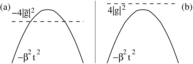
Figure 2: Scattering on a parabolic potential barrier corresponding to the many-body crossing (a, barrier penetration) vs. single-body crossing (b, above-barrier reflection). The dashed line marks the “collision” energy.

A distinction between Eq. (III.57) and the Landau-Zener probability can be clarified by interpretation of the crossing as scattering on a parabolic potential barrier. Indeed Eq. (III.56) can be represented in the form of one-dimensional stationary Schrödinger equation

$$-\ddot{\psi}_{c,s}\left(p,t\right)-\left(\beta^{2}t^{2}-i\beta\right)\psi_{c,s}\left(p,t\right)=-4|\tilde{g}|^{2}\psi_{c,s}\left(p,t\right),$$ (III.58)

where the time plays a role of a coordinate and the “energy’${}^{\prime}{}-4|\tilde{g}|^{2}$ is negative and lies below the the barrier (see Fig. 2a). The sign of the energy is a consequence of antihermiticity of the coupling matrix [see discussion following to Eq. (III.47)]. A single-body curve crossing problem has a hermitian coupling matrix. It can be described by the same Schrödinger equation (III.58) but the energy has an opposite sign and lies above the barrier (see Fig. 2b). Therefore the many-body problem corresponds to barrier penetration with exponentially small penetration probability and large reflection in contrast to large penetration and exponentially small reflection corresponding to single-body crossing. This leads to the replacement of the negative exponents by positive ones, and yields Eq. (III.57) in place of the Landau-Zener formula.

The method of Ref. YBJ02 has been applied to a case of heteronuclear molecules in Ref. KS03 . Exact solutions for some other shapes of $\epsilon_{a}\left(t\right)$ have been obtained using the theory of quantum integrals of motion (see Refs. DM89 and references therein).

III.7 Bose-enhancement and normal density

The effect of Bose enhancement is mathematically expressed as exponentially growing solutions of the equations of motion for the atomic field. Due to equivalence of the parametric approximation and Hartree-Fock-Bogoliubov approach, Eqs. (III.45) have in this case exponentially growing solutions as well. With the neglect of deactivating collisions and of depletion of the molecular field, and for $\epsilon_{p}=$const, the equations for the anomalous and normal densities attain the form of a system of inhomogeneous linear differential equations,

$$i\dot{m}_{s}\left(p,t\right)=2\epsilon_{p}m_{s}\left(p,t\right)+2\tilde{g}^{*}\left[1+2n_{s}\left(p,t\right)\right]$$ (III.59)

$$i\dot{n}_{s}\left(p,t\right)=2\tilde{g}^{*}m^{*}_{s}\left(p,t\right)-2\tilde{g}m_{s}\left(p,t\right).$$ (III.60)

The corresponding homogeneous system has solutions $\sim\exp\left(\pm\kappa t\right)$. The unstable modes with $\epsilon_{p}<2|\tilde{g}|$, or real $\kappa$ [see Eq. (III.54)] demonstrate exponential growth.

Some approximate approaches are based on the neglect of the normal density $n_{s}\left(p,t\right)=0$. In this case Eq. (III.59) has only an oscillating solution $\sim\exp\left(\pm 2i\epsilon_{p}t\right)$ and can not describe the effect of Bose enhancement. As a result such approximations met little success in some situations (see Ref. MSJ02 ). The normal density have to be taken into account also for a correct description of the squeezing of non-condensate atoms (see Sec. VI). Nevertheless, the justified neglect of the normal density in the first-order cummulant approach of Refs. KGB03 ; GKGB04 ; KGG04 ; GKGTJ04 ; GKB05 leads to significant simplification of resulting equations and allows for the description of effects of spatial inhomogeneity beyond the local density approximation. The normal density could be taken into account in higher-order cummulant approaches.

IV Loss of ultracold atoms

The effect of Feshbach resonance in ultracold atomic collisions has been observed at first accompanied by a dramatic loss of trap population when the magnetic field was tuned to the vicinity of the resonance. Such loss has been observed both with atomic BEC IASMSK98 ; SIAMSK99 ; C00 and with ultracold thermal gases M02 .

These experiments can be generally divided to two categories, called in the pioneer MIT works IASMSK98 ; SIAMSK99 as ”slow sweep” and ”fast sweep” ones. In the fast sweep experiments the magnetic field has been ramped through the resonance, while in the slow sweep ones the ramp has been stopped short of crossing. The experiments of the second kind use generally slower ramp speed than the fast sweep ones, or even a static magnetic field, although the principal difference between the two kinds of experiments is the presence or absence of resonance crossing.

The atomic loss is mainly attributed to two loss mechanisms. The first one is a collision-induced deactivation process, such as (I.7) and (I.8) TTHK99 ; YBJW99 ; YBJW00 , undergone by the temporarily formed molecular BEC. The second mechanism involves the molecular dissociation induced by crossing to non-condensate atomic states AV99 ; MTJ00 ; YBJW00 . The effects of the loss mechanisms are non-additive (see Ref. YBJW00 ). An additional loss can be produced by secondary collisions of the relatively hot products of the reactions (I.7) and (I.8) with condensate atoms (see Refs. YBJW99 ; GS99 ; SMASRB01 ).

IV.1 Deactivation loss mechanism

This loss mechanism is included in the mean field approach discussed in Sec. II. Certain properties of the loss process can be described by analytical expressions, obtained from Eq. (II.24), whenever the following “fast decay” conditions hold (see Ref. YBJW00 ):

$$\mu\dot{B}\ll\Gamma_{m}\left(D+\Gamma^{2}_{m}/D\right),\quad\Gamma_{m}\gg\Gamma_{a}$$ (IV.1a)

$$D^{2}+\Gamma^{2}_{m}\gg 6|g|^{2}n_{0}.$$ (IV.1b)

For definitions consult Eqs. (II.25) and (II.26). These conditions mean that the relaxation of $n_{m}$, $v$, and $u$ is much faster compared to that of $n_{0}$ and to the rate of change of the energy, caused by the magnetic field with a ramp speed $\dot{B}$. Therefore the values of the fast variables can be related to a given value of the atomic condensate density $n_{0}$, using a quasi-stationary approximation, by

$$u\sim-{D\over\Gamma{}_{m}}v,\qquad v\sim-{2|g|^{2}n^{2}_{0}\Gamma{}_{m}\over D^{2}+\Gamma{}^{2}_{m}},\qquad n_{m}\sim{|g|^{2}n{}^{2}_{0}\over D^{2}+\Gamma{}^{2}_{m}},$$ (IV.2)

and the condition (IV.1b) leads to $n_{m}\ll n_{0}$. As a result, a single non-linear rate equation for the atomic density can be extracted. When terms proportional to the atomic and molecular densities in $D$ [see Eq. (II.25)] are neglected, the resulting rate equation is

$$\dot{n}_{0}\left({\bf r},t\right)=-{3|g|^{2}k_{a}n^{3}_{0}\left({\bf r},t\right)\over\left[2\epsilon_{a}\left(t\right)+V\left({\bf r}\right)\right]^{2}+\left[k_{a}n_{0}\left({\bf r},t\right)/2\right]{}^{2}}.$$ (IV.3)

(The neglected terms in $D$ effectively add an extra shift to the resonance, but its contribution is hardly noticed in the present problem.)

Equation (IV.3) has a form analogous to the Breit-Wigner expression for resonant scattering in the limit of zero-momentum collisions (see Refs. MTJ00 ; YB03b ). In the Breit-Wigner sense one can interpret $k_{a}n_{0}$ as the width of the decay channel, while the width of the input channel is proportional to $|g|^{2}$. This observation establishes a link between the macroscopic approach used here and microscopic approaches that treat the loss rate as a collision process. However, the right-hand side of Eq. (IV.3) is four times smaller than the usual Breit-Wigner expression. A factor of ${3\over 2}$ is associated with the loss of a third condensate atom in the reaction (I.7), while an additional factor of ${1\over 6}$ is associated with the effects of quantum statistics (see Refs. KSS85 ; B97 ).

IV.1.1 Approaching the resonance

Very close to resonance the behavior of Eq. (IV.3) effectively attains a 1-body form linear in $n$. But as long as we stay out of this narrow region, by obeying the “off-resonance” condition ,

$$k_{a}n\left({\bf r},t\right)\ll|V\left({\bf r}\right)-\mu B\left(t\right)|,$$ (IV.4)

we can write Eq. (IV.3) (to a very good approximation) in the 3-body form

$$\dot{n}_{0}=-3K_{3}\left({\bf r},t\right)n^{3}_{0},\qquad K_{3}={2\pi|a_{a}|k_{a}\Delta\over m\mu\left[B\left(t\right)-B_{0}-V\left({\bf r}\right)/\mu\right]{}^{2}}.$$ (IV.5)

The three-body rate coefficient $K_{3}$ is defined here according to conventional chemical notation. It is three times less then the one in Refs. YBJW99 ; YBJW00 ; SIAMSK99 . The dependence of Eq. (IV.5) on the scattering length $a_{a}$ follows from Eq. (II.21).

The above results are obtained neglecting the atomic transport described by the kinetic energy terms in Eq. (II.20). This approximation is valid while the characteristic times are small compared to the trap periods. A different situation takes place in the slow-sweep experiments IASMSK98 ; SIAMSK99 , where the characteristic sweep times are large compared to the trap periods, and the atomic transport has time to restore the Thomas-Fermi distribution. In this case the averaging of Eq. (IV.5) over the distribution (II.28) leads to the following rate equation

$$\dot{\bar{n}}=-3{50\over 21}K_{3}\left({\bf r},t\right)\bar{n}^{3}$$ (IV.6)

for the mean BEC density $\bar{n}\left(t\right)={2\over 5}n_{\text{peak}}\left(t\right)$.

When the magnetic field ramp is assumed to vary linearly in time, starting at $t_{0}$ and ending at $t$, and Eq. (IV.4) applies throughout the ramp motion (i.e., by avoiding passage through the resonance as in the slow sweep experiments), this rate equation can be solved analytically as,

$$\bar{n}\left(t\right)=\bar{n}\left(t_{0}\right)\left[1+{200\over 7}\pi|a_{a}|k_{a}\bar{n}^{2}\left(t_{0}\right)\Delta{t-t{}_{0}\over m\mu\dot{B}^{2}t_{0}t}\right]^{-1/2},$$ (IV.7)

where $\dot{B}$ is the magnetic-field ramp speed and the extrapolated time of reaching exact resonance is chosen to be $t=0$, so that both $t$ and $t_{0}$ have the same sign. A similar expression for the homogeneous case has been presented in Refs. YBJW99 ; YBJW00 . Figure 3 demonstrates a reasonably good agreement between the model and experimental data of Ref. SIAMSK99 for the 907 G resonance in ²³Na. The model uses the parameter values $\Delta=0.98$ G, $a_{a}=3.4$ nm, and $\mu=3.65\mu_{B}$, calculated in Ref. MTJ00 , and $k_{a}=5.5\times 10^{-11}$cm${}^{3}/$s, measured in Ref. MAXCK04 , and does not contain adjustable parameters.

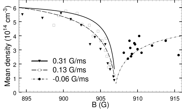
Figure 3: The surviving mean density (see Eq. (IV.7) vs. the stopping value of the magnetic field. The resonance was approached from below with two ramp speeds, 0.13 G/s and 0.31 G/s, or from above, with the ramp speed -0.06 G/s. These are compared with the experimental results SIAMSK99 (squares, triangles and circles).

IV.1.2 Passing through the resonance

The off-resonance approximation of Eqs. (IV.4) and (IV.5) does not hold very close to resonance, and is therefore inapplicable to the description of the fast-sweep experiment, in which the Zeeman shift is swept rapidly through the resonance, causing dramatic losses. Nevertheless, the fast decay approximation (IV.1) may still be valid. A simple analytical expression can then be derived for the condensate loss on passage though the resonance if, in addition, the magnetic field variation lasts long enough to reach the “asymptotic” condition

$$\mu\delta B\gg k_{a}n_{0},$$ (IV.8)

where $\delta B$ is the total change in $B$ accumulated over the sweep. This condition allows the extension of the ramp starting and stopping times to $\mp\infty$.

One can now evaluate the variation of $n_{0}\left({\bf r},t\right)$ in the infinite time interval $\left(-\infty,\infty\right)$. Let us rewrite Eq. (IV.3) in the form

$${dn_{0}\left({\bf r},t\right)\over n^{2}_{0}\left({\bf r},t\right)}=-{3k_{a}n_{0}\left({\bf r},t\right)|g|{}^{2}\over\left(\mu\dot{B}t\right)^{2}+\left(k_{a}n_{0}\left({\bf r},t\right)/2\right){}^{2}}dt,$$ (IV.9)

where $V\left({\bf r}\right)$ is removed by our choice of the origin on the time scale. We then integrate the left-hand side with respect to $n_{0}$ from $n_{0}\left({\bf r},-\infty\right)$ to $n_{0}\left({\bf r},\infty\right)$ and the right-hand side with respect to $t$ from $-\infty$ to $\infty$, considering $n_{0}$ as a well-defined function of $t$. The latter integral may be evaluated by using the residue theorem, closing the integration contour by an arc of infinite radius in the upper half-plane. The integral along this arc vanishes according to the asymptotic behavior of $n_{0}$ (see Ref. YBJW00 ).

The final result does not depend on $k_{a}$ and has the form (valid for all positions ${\bf r}$)

$$n_{0}\left({\bf r},\infty\right)={n_{0}\left({\bf r},-\infty\right)\over 1+sn_{0}\left({\bf r},-\infty\right)},\qquad s={6\pi|g|{}^{2}\over\mu|\dot{B}|}={12\pi^{2}|a_{a}|\over m}{\Delta\over|\dot{B}|}.$$ (IV.10)

The product $sn_{0}$ in Eq. (IV.10) would be proportional to the Landau-Zener exponent for the transition between the condensate and the resonant molecular states whose energies cross due to the time variation of the magnetic field, if one could keep the coupling strength $g\varphi_{0}$ constant. However, for the non-linear curve crossing problem represented by Eq. (II.20), the Landau-Zener formula is replaced by Eq. (IV.10), which predicts a lower crossing probability, since the coupling strength $g\varphi_{0}$ decreases, along with the decrease of the condensate density during the process. The transition probability in the Landau-Zener model with relaxation, obtained in Ref. DOS76 , is given by the same Landau-Zener formula, as in the absence of the relaxation, and is independent of the relaxation rate as well as Eq. (IV.10). However, unlike the Landau-Zener formula, Eq. (IV.10) is applicable only at strong relaxation, when the fast decay approximation is valid.

The asymptotic result (IV.10) describes the decay of the condensate density. Assuming a homogeneous initial density within the trap, Eq. (IV.10) applies also to the loss of the total population $N_{0}\left(t\right)=\int n_{0}\left({\bf r},t\right)d^{3}r$. An asymptotic expression for the total population can also be found when the homogeneous distribution is replaced by the Thomas-Fermi one [see Eq. (II.28)]. In this case, given $n_{\text{peak}}$ is the maximum initial density in the center of the trap, one obtains

$${N_{0}\left(\infty\right)\over N_{0}\left(-\infty\right)}={15\over 2sn{}_{\text{peak}}}\left({1\over 3}+{1\over sn{}_{\text{peak}}}-{1\over 2sn{}_{\text{peak}}}\sqrt{1+{1\over sn{}_{\text{peak}}}}\ln{\sqrt{1+{1\over sn{}_{\text{peak}}}}+1\over\sqrt{1+{1\over sn{}_{\text{peak}}}}-1}\right).$$ (IV.11)

Figure 4: Schematic illustration of transitions between atomic and molecular condensates and non-condensate atoms on a forward sweep.

IV.2 Dissociation loss

The consideration above did not include the decay of the resonant molecular state by transferring atoms to excited (discrete) trap states or to higher-lying non-trapped (continuum) states. In a forward sweep, when the molecular state crosses the atomic ones upwards (see Fig. 4), this process can be described by curve-crossing theory as a sequence of two-state crossings.

Consider the system in a normalization box of volume ${\cal V}$. The number of states of a pair of atoms with momenta ${\bf p}$ and $-{\bf p}$ per unit of the energy $\epsilon=p^{2}/m$ of their relative motion is

$$\nu_{\epsilon}={{\cal V}\over 4\pi{}^{2}}m^{3/2}\epsilon^{1/2}.$$ (IV.12)

Due to the time variation of the magnetic field, the molecular state crosses at the time $t$ the atomic pair state with the energy $\epsilon=-2\epsilon_{a}\left(t\right)=\mu\left(B\left(t\right)-B_{0}\right)$, altogether crossing $\nu_{\epsilon}\mu\dot{B}$ such states per unit time. If the depletion of the molecular field during each crossing can be neglected, the crossings can be described by the many-body curve-crossing model of Sec. III.6. The number of atoms formed by each crossing is determined by Eq. (III.57), with

$$\lambda={8\pi|a_{a}|\Delta\over m|\dot{B}|}n_{m}.$$ (IV.13)

Therefore, the loss rate of the molecular population is

$$\dot{N}_{m}=-{1\over 2}\left(1-e^{-2\pi\lambda}\right)e^{2\pi\lambda}\nu_{\epsilon}\mu\dot{B}.$$ (IV.14)

If the molecular density is small enough, such that $\lambda\ll 1$, one obtains a loss rate of the molecular density

$$\dot{n}_{m}\approx-2\Gamma_{\text{dis}}n_{m},\qquad\Gamma_{\text{dis}}=|a_{a}\mu|\Delta\sqrt{m\mu\left(B\left(t\right)-B_{0}\right)},$$ (IV.15)

which is proportional to the dissociation width $\Gamma_{\text{dis}}$. The same result can be obtained by using of Landau-Zener theory (see Ref. YBJW00 ). Therefore one can account for the decay of the resonant molecular state into excited trap states by adding a term $-i\Gamma_{\text{dis}}\varphi_{m}$ to the right hand side of Eq. (II.20b). This approach is in good agreement with the parametric approximation only whenever (a) the variation of the molecular field during each crossing is negligible; and (b) $\lambda\ll 1$ and the quantum effect of Bose enhancement, described by the positive-exponential factor in Eq. (IV.14), is negligible (see Secs.  III.6 and III.7). These conditions are obeyed with the parameters used in the calculations of Ref. YBJW00 for the Na resonances , the results of which are confirmed by using the parametric approximation. For example, Fig. 5 compares the two approximate methods for the Na resonance at 853 G with the strength $\Delta\approx 9.5$ mG (see Ref. MTJ00 , other parameters having the same values as for the 907 G resonance presented at the end of Sec. IV.1.1).

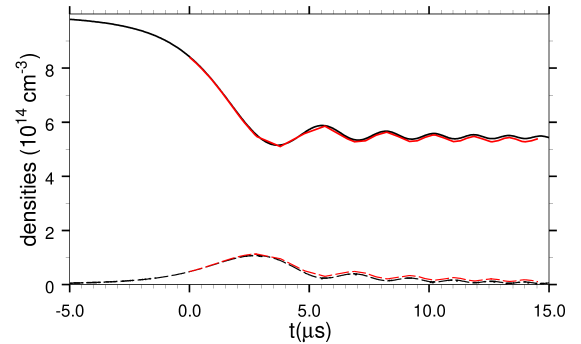
Figure 5: Time dependence of the densities of the atomic (solid lines) and molecular (dashed lines) condensates calculated for the Na resonance at 853 G using the parametric approximation (black lines) and the mean-field approach taking into account the dissociation width $\Gamma_{\text{dis}}$ (red lines).

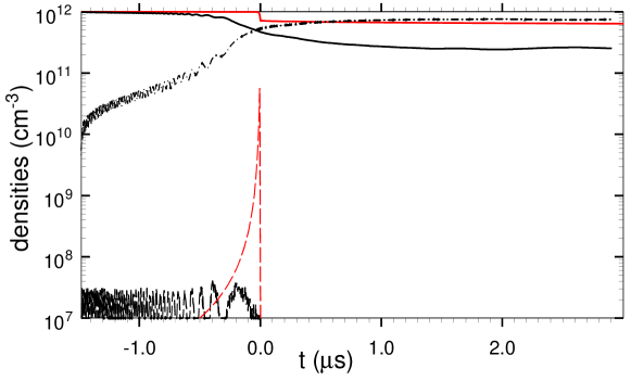
Figure 6: Time dependence of the densities of the atomic (solid lines) and molecular (dashed lines) condensates calculated for the ⁸⁵Rb resonance using the parametric approximation (black lines) and the mean-field approach taking into account the dissociation width $\Gamma_{\text{dis}}$ (red lines). The dot-dashed line plots the density of non- condensate atoms calculated using the parametric approximation. The ramp speed is $\dot{B}=5$ G/ms.

However, under other conditions the two methods produce different results. Figure 6 compares them for a case of ⁸⁵Rb resonance (see Ref. YB03j ). The values of $\Delta=11$ G, $B_{0}=154.9$ G, and $a_{a}=-450$ (in atomic units) are taken from Ref. D02 , and the value of $\mu=-2.23\mu_{\text{B}}$ is taken from Ref. KH02 . The condensate loss calculated with the parametric approximation is more then two times higher then the one calculated with the mean field approach. The main loss mechanism is the Bose-enhanced crossing to the non-condensate atomic states. The Bose-enhanced dissociation drastically reduces the molecular condensate density, compared to the mean field results, leading to the suppression of deactivation losses (the total density of condensate and non-condensate atoms remaining almost unchanged and the results are insensitive to deactivation rates for $k_{a},k_{m}<10^{-8}$cm${}^{3}/$s). As a result, the parametric approximation demonstrates a much better agreement with the experimental data than the mean field results (see Fig. 7). The drastic increase of loss at slower sweeps is actually related to the effect of Bose-enhancement, as demonstrated by the plot for the maximal value of the non-condensate state occupation $n_{s}\left(p,t\right)$ in Fig. 7. The disagreement between the parametric approximation and the experimental data at intermediate ramp speeds can be related to fluctuations of the molecular field and higher-order correlations of the atomic field neglected in both theories.

Figure 7: Loss of atomic condensate (solid line) and maximal non-condensate state occupation (dashed line) as a function of inverse ramp speed calculated using the parametric approximation in comparison with the experimental data by Cornish et al. C00 (circles). The dot-dashed and dotted lines demonstrate, respectively, the results of mean-field calculations taking into account the dissociation width $\Gamma_{\text{dis}}$ and without this account for $k_{a}=2\times 10^{-9}$ cm${}^{3}/$s.

It is interesting that the inclusion of the dissociation loss mechanism reduces the total loss (cf. the dotted and dot-dashed lines in Fig.. 7). This paradoxical result has the following explanation. The coupling to non-condensate atom continuum shifts the molecular state energy (above the continuum threshold the shift is imaginary and proportional to the width). The energy-dependent shift effectvely accelerates the sweep, reducing the probability of crossing from the atomic to molecular BEC. For weaker resonances, when the crossing probability remains almost unchanged, an additional effect becomes most prominent (see Ref. YBJW00 ). The atom-molecule deactivation (I.7) leads to the loss of three condensate atoms per each resonant molecule formed, while the dissociation leads to the loss of only two condensate atoms. Therefore, the inclusion of dissociation losses transfers flow from the deactivation (I.7) to the dissociation, thus reducing the number of condensate atoms lost per each resonant molecule formed. By the same reason in a case of small dissociation loss, the increase of molecule-molecule deactivation rate coefficient reduces the total loss (see calculations for Na in Ref. YBJW00 ).

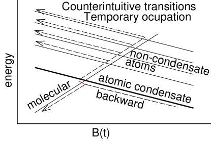
Figure 8: Schematic illustration of transitions between atomic and molecular condensates and non-condensate atoms on a backward sweep.

V Formation of molecules

In the experiments HKMWCNG03 ; MKHCNG04 ; DVMR03 ; DVMR04 ; XMACMK03 ; MAXCK04 diatomic molecules have been formed by sweeping the Zeeman shift through resonance in a backward direction, so that the molecular state crossed the atomic ones downwards (see Fig. 8). This led to the transfer of population from the lowest atomic (condensate) state to the molecular state, as had been proposed in Ref. MTJ00 . In a backward sweep, unlike the forward one (see Fig. 4), the transitions to non-condensate atomic states are forbidden in semiclassical Landau-Zener-type theories (see Refs. ChildMCT ; NU84 ; DO88 ; Akulin05 ) as the second crossing, from the molecular to a non-condensate atomic state, precedes in time the first one, from the atomic to the molecular condensate state. Nevertheless, quantum theory allows the non-condensate states to be populated temporarily by so-called “counterintuitive transitions” (see Ref. counter_int ), which are most notable in strong resonances or at low densities (see Ref. YB03 ). The molecules are also lost due to deactivating collisions with atoms or other molecules (I.7) and (I.8). Therefore, an adequate analysis of molecular formation requires a quantum many-body theory that takes into account relaxation, such as the parametric approximation.

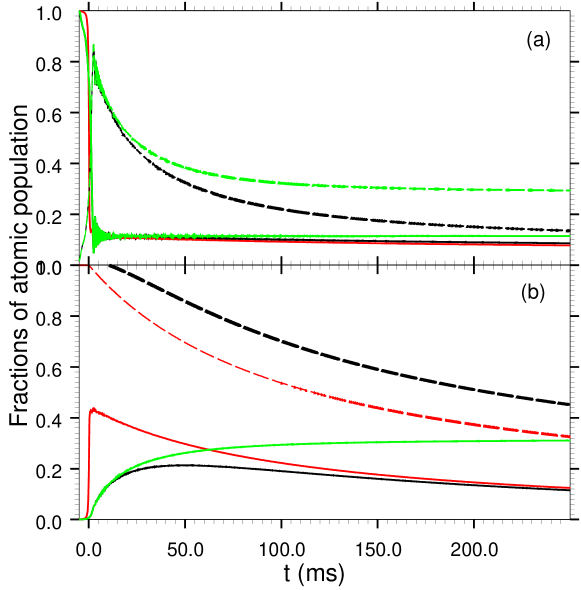
Figure 9: Results of calculations for the 1007 G resonance in ⁸⁷Rb using the parametric approximation with deactivation (black lines) and without it (green lines). The red lines plot the mean-field results. Part (a) presents the fractions of the atomic populations surviving in the condensate form (solid lines) and converted to non-condensate atoms (dashed lines). The fractions of atomic population converted to molecules are plotted by the solid lines in the part (b), while the dashed lines plot the sum of all atomic and twice molecular populations. All plots are calculated for the initial atomic density $10^{11}$ cm^-3 and the ramp speed of 1 G/s in a backward sweep.

Figure 9 compares various approximations for the case of the 1007 G resonance in ⁸⁷Rb. The parameter values $\Delta=0.2$ G and $a_{a}=99$ atomic units have been measured in Ref. VDEMR03 , $\mu=2.8\mu_{B}$ has been calculated in Ref. M02 , and $k_{a}=7\times 10^{-11}$ cm${}^{3}/$s has been estimated in Ref. YB03b . The molecule-molecule deactivation rate coefficient is estimated here as $k_{m}=10^{-10}$cm${}^{3}/$s.

The results of calculations using the parametric approximation demonstrate that the temporary non-condensate atom population persists during a time comparable to the deactivation time. This population substantially reduces the maximal molecular density and shifts the maximum time compared to the mean-field results. This difference is less pronounced in the case of the weaker 685 G resonance (see Fig. 10), with $\Delta=17$ mG, $\mu=1.4\mu_{\text{B}}$ (see Ref. M02 , other parameters are the same as for the 1007 G resonance).

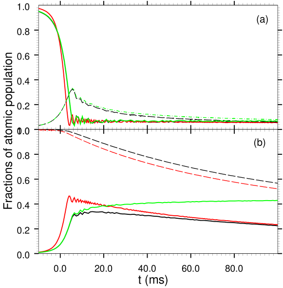
Figure 10: Same as in Fig. 9, but for the 685 G resonance in ⁸⁷Rb and the ramp speed of 0.05 G/s.

Figures 9 and 10 contain also results of parametric calculations neglecting the deactivation losses ($k_{a}=k_{m}=0$). In this case the molecular density increases monotonically in time due to the association of non-condensate atoms, while the atomic density remains almost unchanged.

The conversion efficiency $2\max\left(n_{m}\left(t\right)\right)/n_{0}\left(t_{0}\right)$ is determined by a concurrence of three processes: the association of the atomic condensate and the two loss processes — the dissociation of the molecular BEC onto non-condensate atoms and the deactivation by inelastic collisions. A qualitative behavior of the conversion efficiency can be analyzed using the rescaled equation Eq. (III.43). The first term in the right-hand side is related to association, the second one — to dissociation, and the rest — to deactivation. The problem depends on the parameter $\sigma$ [see Eq. (III.44)], the scaled deactivation rate coefficients $\tilde{k}_{a,m}$, and a scaled ramp speed, which can be expressed as $\left(sn\right)^{-1}$ in terms of the parameter $s$ defined in Eq. (IV.10). Given the rescaled ramp speed, an increase of the resonance strength $\Delta$ increase the parameter $\sigma$ [see Eq. (III.44)] and, therefore, the dissociation term in Eq. (III.43), but decrease the deactivation rates proportional to $\tilde{k}_{a,m}$ [see Eq. (III.42)]. A decrease of the atomic density has the same effect.

The part of associated atomic condensate increases with decrease of the ramp speed, saturating at values of $sn\sim 1$ [see Eq. (IV.10) and the following discussion]. The molecular loss is proportional to the time and, therefore, it is inverse proportional to the ramp speed. This leads to the existence of an optimal ramp speed $\dot{B}\propto n\Delta$.

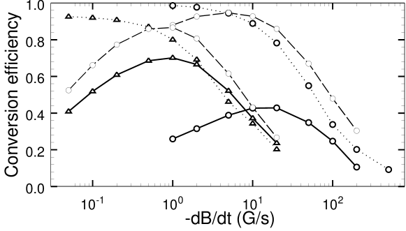
Figure 11: Conversion efficiency as a function of the ramp speed calculated for the 1007 G (circles) and 685 G (triangles) resonances in ⁸⁷Rb with the initial atomic density of $10^{12}$ cm^-3 using the parametric approximation with deactivation (solid lines) and without it (dotted lines). The dashed lines plot the mean-field results.

This qualitative analysis is confirmed by results of numerical calculations (see Figs. 11 and 12). The maximum in the ramp-speed dependence is not reproduced by calculations neglecting the deactivation. The mean-field calculations predict the maximum, but overestimate the conversion efficiency and provide a slower optimal ramp speed, especially for the stronger resonance (see Fig. 11). The conversion efficiency at the optimal ramp speed decreases at high densities due to deactivation and at low densities due to non-condensate atom population (see Fig. 12), reaching a maximum at the density $10^{12}$ cm^-3 for the weaker 685 G resonance. In the case of the stronger 1007 G, resonance the non-condensate atom population is the dominant loss process in the full range of densities considered here, and the conversion efficiency remains almost unchanged, slightly increasing with the density.

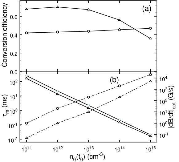
Figure 12: (a) conversion efficiency and (b) the lifetime of the molecular condensate $\tau_{m}$ (solid lines) at the optimal ramp speed $\left(dB/dt\right)_{\text{opt}}$ (dashed lines), all plotted as functions of the initial atomic density $n_{0}\left(t_{0}\right)$, calculated with the parametric approximation, for the resonances at 1007 G (circles) and 685 G (triangles) in ⁸⁷Rb.

The low density required for a more effective conversion can be achieved by the use of expanding condensates, as in experiments HKMWCNG03 ; MKHCNG04 ; DVMR03 ; DVMR04 . In the ⁸⁷Rb experiments DVMR03 ; DVMR04 , the magnetic field ramp was started after a preliminary expansion interval $t_{p}\geq 2$ ms, following the switching off of the trap. In this case the analysis can be satisfactorily carried out by using the mean-field approach (see Ref. YB04 and Sec. II.3). This is demonstrated by Fig. 13, comparing the atomic and molecular densities calculated with the parametric approximation to those calculated with the mean field approach, under the appropriate conditions. The initial atomic density used corresponds to the mean density reached at the expansion time of 2 ms. As one can see, already when the magnetic field is just 0.5 G below the resonance (in a sweep totaling 2.2 G), the results of the two kinds of calculations coincide. When faster magnetic sweeps or higher densities are considered, the results of the two approaches converge even faster.

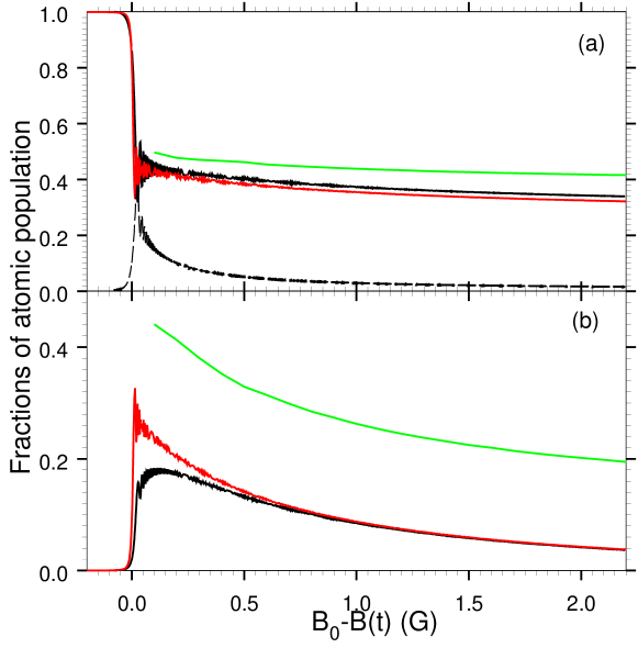
Figure 13: Fraction of atomic population surviving in the atomic condensate (a) and converted to molecules (b), calculated using the parametric approximation (black lines) and the mean field approach (red lines), for the 1007 G resonance in a homogeneous ⁸⁷Rb BEC with an initial atomic density $2\times 10^{13}$cm^-3 and a magnetic ramp speed of 1 G/ms. The fraction of non-condensate atoms calculated with the parametric approximation is represented by the dashed line in part (b). The green lines represent the fraction of surviving and converted population calculated using the mean field approach while taking account of spatial inhomogeneity and expansion.

The applicability of the mean-field approach at the experimental conditions allows us to analyze the case of an expanding condensate using a numerical solution of Eqs. (II.37) and (II.38) (see Fig. 13). The expansion reduces the atomic density, leading to a slower loss of atoms and molecules. The results are in agreement with the experimental data of Ref. DVMR03 reporting that $\sim 7\%$ of the atoms are converted to molecules and $\sim 30\%$ remain in the atomic condensate for ramp speeds of less than 2 G/ms.

VI Formation of entangled atoms

The dissociation of the molecular BEC in a forward sweep (see Fig. 4) has been considered in Sec. IV as one of the loss mechanisms. However, the dissociation is not just an undesirable process, since the molecules dissociate to entangled pairs of atoms with opposite momenta (see Ref. YB03 ), as in the case of an unstable atomic BEC (see Ref. Y02 ). Indeed, substitution of the molecular mean field (III.2) into the atom-molecule coupling (I.21) leads to an interaction proportional to a product of atomic field operators with opposite momenta. Interactions of similar form are known in the theory of parametric down conversion in quantum optics (see Refs. SZ97 ; BR97 ). Likewise, the atoms are formed in two-mode squeezed states, which are similar to the state of electromagnetic radiation formed by parametric down conversion.

In order to clarify the nature of this entanglement, let us write out a pseudo-Hamiltonian

$$\hat{H}_{a}=\sum\limits_{p_{z}>0}\hat{H}\left({\bf p},t\right),$$ (VI.1)

that leads to equations of motion for the atomic field (III.11), expressed as a sum of contributions of different momentum modes in a normalization box,

$$\hat{H}_{a}\left({\bf p},t\right)=\left[{p{}^{2}\over 2m}+\epsilon_{a}\left(t\right)-i{k{}_{a}\over 2}|\varphi_{m}\left(t\right)|^{2}\right]\left[\hat{\Psi}^{{\dagger}}_{a}\left({\bf p},t\right)\hat{\Psi}_{a}\left({\bf p},t\right)+\hat{\Psi}^{{\dagger}}_{a}\left(-{\bf p},t\right)\hat{\Psi}_{a}\left(-{\bf p},t\right)\right]$$

$$+\biggl{\{}2\tilde{d}_{h}\left(2p\right)\varphi^{*}_{m}\left(t\right)\hat{\Psi}_{a}\left({\bf p},t\right)\hat{\Psi}_{a}\left(-{\bf p},t\right)+i\hat{F}\left({\bf p},t\right)\left[\hat{\Psi}^{{\dagger}}_{a}\left({\bf p},t\right)+\hat{\Psi}^{{\dagger}}_{a}\left(-{\bf p},t\right)\right]+\mathrm{h.c.}\biggr{\}}.$$

Although the pseudo-Hamiltonian is not hermitian, it allows writing the time evolution operator in the form

$$\hat{\Omega}\left(t\right)=\prod_{p_{z}>0}\hat{\Omega}\left({\bf p},t\right),$$ (VI.2)

where (using the time-ordering operator $T$)

$$\hat{\Omega}\left({\bf p},t\right)=T\exp\left(-i\int\limits^{t}_{t{}_{0}}\hat{H}_{a}\left({\bf p},t^{\prime}\right)dt^{\prime}\right).$$ (VI.3)

The representation of the operator $\hat{\Omega}\left(t\right)$ as a product of single-mode operators $\hat{\Omega}\left({\bf p},t\right)$ follows from the commutativity of the $\hat{H}_{a}\left({\bf p},t\right)$ with different values of ${\bf p}$.

Imagine a measurement, represented by a projection operator $\hat{P}\left({\bf p}\right)$, which selects atoms with the momentum ${\bf p}$ moving in the positive $z$-direction, and does not affects atoms moving in the negative $z$-direction. This measurement reduces the state vector $\hat{\Omega}\left(t\right)|$in$\rangle$ to $\hat{P}\left({\bf p}\right)\hat{\Omega}\left(t\right)|$in$\rangle=\hat{\Omega}\left({\bf p},t\right)|$in$\rangle$. The distribution of atoms moving in the negative $z$-direction (the average number of atoms with the momentum ${\bf p}^{\prime}$) after this measurement will be determined by

$$\langle\text{in}|\hat{\Omega}^{{\dagger}}\left(t\right)\hat{\Psi}^{{\dagger}}_{a}\left({\bf p}^{\prime},t\right)\hat{\Psi}_{a}\left({\bf p}^{\prime},t\right)\hat{\Omega}\left({\bf p},t\right)|\text{in}\rangle\propto\delta_{-{\bf p}{\bf p}^{\prime}},$$ (VI.4)

representing an entanglement of atoms with opposite momenta. This analysis is similar to the one used in the entanglement of the signal and the idle in the process of degenerate two-photon down-conversion in quantum optics (see Refs. SZ97 ; BR97 ). The state of atoms is also perfectly number-squeezed, i. e. it has zero variance in the relative number of atoms with opposite momenta, as in the case considered in Ref. RGB02 .

As demonstrated in YBJ02 the non-condensate atoms produced by molecular dissociation are formed in squeezed states, which now turn out to be two-mode squeezed states, as in Y02 . As in quantum optics, the squeezing is related to the quadrature operators

$$\hat{X}\left({\bf p},t\right)={1\over 2}\Bigg{\{}\left[\hat{\Psi}_{a}\left({\bf p},t\right)\pm\hat{\Psi}_{a}\left(-{\bf p},t\right)\right]e^{i\theta}+\left[\hat{\Psi}^{{\dagger}}_{a}\left({\bf p},t\right)\pm\hat{\Psi}^{{\dagger}}_{a}\left(-{\bf p},t\right)\right]e^{-i\theta}\Biggr{\}}.$$ (VI.5)

The uncertainties of the quadratures can be written out as

$$\langle\text{in}|\hat{X}\left({\bf p}_{1},t\right)\hat{X}\left({\bf p}_{2},t\right)|\text{in}\rangle={1\over 2}\delta\left({\bf p}_{1}-{\bf p}_{2}\right)\left\{1+2n_{s}\left(p,t\right)\pm 2\text{Re}\left[m_{s}\left(p,t\right)e^{2i\theta}\right]\right\}$$ (VI.6)

where the momentum spectra $n_{s}\left(p,t\right)$ and $m_{s}\left(p,t\right)$ are defined by Eqs. (III.29) and (LABEL:Anden), respectively.

The uncertainties attain maximal and minimal values at two orthogonal values of the phase angle $\theta$. The amount of squeezing can be quantified by the energy-dependent parameter

$$r\left(\epsilon,t\right)={1\over 4}\ln{\langle\text{in}|\hat{X}\left({\bf p}_{1},t\right)\hat{X}\left({\bf p}_{2},t\right)|\text{in}\rangle{}_{\max}\over\langle\text{in}|\hat{X}\left({\bf p}_{1},t\right)\hat{X}\left({\bf p}_{2},t\right)|\text{in}\rangle{}_{\min}}={1\over 4}\ln{1+2n_{s}\left(p,t\right)+2|m_{s}\left(p,t\right)|\over|1+2n_{s}\left(p,t\right)-2|m_{s}\left(p,t\right)||}.$$ (VI.7)

A mean squeezing parameter, weighed by the spectral density of Eq. (III.34),

$$\bar{r}\left(t\right)=\int dE\tilde{n}_{s}\left(E,t\right)r\left(E,t\right)/n_{s}\left(t\right).$$ (VI.8)

is used to describe the time variation of the squeezing.

In the case of a rather weak resonance a description of the dissociation of a pure molecular BEC can be attempted by a simple analytical model based on the approach of Sec. IV.2 (see also Refs. MAXCK04 ; GKGTJ04 ; YB04 ). The molecular density is given by the solution of Eq. (IV.15),

$$n_{m}\left(t\right)=n_{m}\left(t_{d}\right)\exp\left[-2|a_{a}\mu|\Delta\int\limits^{t}_{t{}_{d}}dt^{\prime}\sqrt{m\mu\left(B\left(t^{\prime}{}\right)-B_{0}\right)}\right],$$ (VI.9)

where $t_{d}$ is the time of start of the dissociating ramp. A molecule dissociates into two entangled atoms, each with an energy $E$, by a crossing occurring at $\mu\left(B\left(t\right)-B_{0}\right)=2E$. The resulting energy distribution of the formed atoms can be written out as

$$\tilde{n}_{s}\left(E\right)={1\over 2}\sqrt{E}E^{-3/2}_{\text{peak}}\exp\left[-{1\over 3}\left(E/E_{\text{peak}}\right)^{3/2}\right],$$ (VI.10)

where

$$E_{\text{peak}}={1\over 2m}\left({m|\dot{B}|\over 4|a_{a}|\Delta}\right)^{2/3}$$ (VI.11)

is the peak energy. Although the model does not produce the correct molecular density dynamics (see Fig. 14a), it gives a surprisely good agreement with the numerical results for the energy distribution (see Fig. 14b). The analytical model demonstrates also a very good agreement to experimental data, as reported in Refs. MAXCK04 ; DVMR04 . It should be noted that at high energy Eqs. (III.29), (III.35), and (III.38) lead to $\tilde{n}_{s}\left(E\right)\propto E^{-3/2}$. Therefore, the distribution has a divergent mean energy. The peak energy (VI.11) is well defined for each distribution. It is proportional to the mean energy for the distribution (VI.10) used in Refs. MAXCK04 ; DVMR04 .

Figure 14: (a) Fraction of surviving molecular population calculated by using Eq. (VI.9) (solid line) and by the parametric approximation for the initial molecular density $n_{m}\left(t_{d}\right)=10^{10}$ cm^-3(dotted line), $10^{11}$ cm^-3(dot-dashed line), and $10^{12}$ cm^-3(dashed line). (b) Energy distribution calculated by using Eq. (VI.10) (solid line) and the parametric approximation for the initial molecular density $10^{11}$ cm^-3 ($\times$) and $10^{12}$ cm^-3(+).

In the case of molecular condensate dissociation the squeezing parameter does not exceed the value of $r=0.35$ even for the initial molecular density of $10^{12}$ cm^-3. The nature of such low squeezing can be understood by using the exactly soluble many-body curve-crossing model of Sec. III.6. Using expressions for the uncertainties of the quadrature operators (VI.5) derived in Ref. YBJ02 , one can represent the squeezing parameter (VI.7) as

$$r={1\over 2}\ln{\left(e^{2\pi\lambda}-1\right)^{1/2}+e{}^{\pi\lambda}\over|\left(e^{2\pi\lambda}-1\right)^{1/2}-e^{\pi\lambda}|},$$ (VI.12)

where the Landau-Zener parameter $\lambda$ is defined by Eq. (IV.13). In the case of $\lambda\ll 1$, when Eqs. (VI.9) and (VI.10) are applicable [see discussion following to Eq. (IV.15)], the squeezing parameter is $r\approx\sqrt{2\pi\lambda}\ll 1$. In the opposite case of $\lambda\gg 1$, Eq. (VI.12) relates the squeezing parameter to the occupation of the non-condensate mode $n_{s}\left(p,t\right)\approx e^{2\pi\lambda}$ [see Eq. (III.57] as $r={1\over 2}\ln\left(4n_{s}\right)$, in agreement with an exact relation $n_{s}=\sinh^{2}r$, derivable from the definition of squeezed states (see Refs. SZ97 ; BR97 ). This relation between high squeezing and high mode occupation demonstrates that a correct calculations of the entangled atomic pair properties require taking into account the normal density.

Figure 15: (a) Time dependence of the densities of the atomic condensate (dotted line), entangled atoms (solid line), and the molecular condensate (dot-dashed line, $\times 10^{3}$) calculated for the 685 G resonance in ⁸⁷Rb with the initial atomic density $10^{13}$ cm^-3 and a ramp speed of 20 G/s in a forward sweep. The dashed line shows the mean squeezing parameter $\bar{r}\left(t\right)$ [see Eq. (VI.8)]. (b) Energy spectra of the entangled-atom density $\tilde{n}_{s}\left(E,t\right)$ (solid line) and the squeezing parameter $r\left(E,t\right)$ (dashed line) calculated at $t\approx 23$ ms.

Higher squeezing can be obtained on dissociation of molecules formed temporarily from the atomic BEC on a forward sweep (see Fig. 4). In this case (see Fig. 15) the molecular density is very low (about $10^{10}$ cm^-3) and persists a shorter time (compared to that in the backward sweep) due to fast dissociation, leading to a negligibly small deactivation loss. Figure 15a demonstrates almost full transformation of the atomic BEC into a gas of entangled atomic pairs in two-mode squeezed states with the mean squeezing parameter $\bar{r}\approx 2.4$, corresponding to a noise reduction of about 20 dB. The energy spectra of the entangled-atom density and the squeezing parameter are presented in Fig. 15b. The density spectra are rather narrow, and the peak energy increases with time. The squeezing parameter reaches the value of $r\left(E,t\right)\approx 3.4$ (corresponding to noise reduction of about 30 dB) for the mode with occupation $n_{s}\approx 240$ at the energy $E\approx 1$ nK. Comparable squeezing of $\max r\left(E,t\right)\approx 3.6$ have been calculated in Ref. YB03 for the 853 G resonance in Na. These values substantially exceed $\max r\left(E,t\right)\approx 1.4$ calculated in Ref. YB03j for the much stronger resonance in ⁸⁵Rb.

Conclusion

A correct theoretical treatment of Feshbach resonance in BEC has to take into account both quantum fluctuation (formation of non-condensate atoms) and damping due to deactivation of the resonant molecules in inelastic atom-molecule and molecule-molecule collisions. The deactivating collisions lead to condensate loss and the limitation of the atom-molecule conversion efficiency at high densities and slow sweeps. The quantum fluctuations of the atomic field describe Bose-enhanced condensate losses, the limitation of atom-molecule conversion efficiency at low densities, and the formation of entangled atomic pairs in two-mode squeezed states. The effects of fluctuations and deactivation on the loss are non-additive. The squeezing and Bose-enhancement of non-condensate atom formation can be described by second-order correlations, but only if both normal and anomalous densities are taken into account.

The parametric approximation takes into account both the damping and fluctuations in a proper way. This method gives analytical solutions for some model systems and can be used for numerical calculations in more general cases. The results of numerical calculations generally agree with the experimental data and provide optimal conditions for atom-molecule conversion and quantum properties of entangled atoms.

References

- (1) Parkins, A.S.; Walls, D.F. Phys. Rep. 1998,303, 1-80.
- (2) Dalfovo, F.; Giorgini, S.; Pitaevskii, L.P.; Stringari, S. Rev. Mod. Phys. 1999, 71, 463-512.
- (3) Courteille, Ph. W.; Bagnato, V. S.; Yukalov, V. I. Laser Phys. 2001, 11, 659-800.
- (4) Rogel-Salazar, J.; Choi, S.; New, G. H. C.; Burnett, K. J. Opt. B 2004, 6, R33-R59.
- (5) Yukalov, V. I. Laser Phys. Lett. 2004, 1, 435-462.
- (6) Pitaevskii, L.P.; Stringari, S. Bose-Einstein Condensation in Dilute Gases; Cambridge University Press: Cambridge, MA, 2002.
- (7) Herbig, J.; Kraemer, T.; Mark, M.; Weber, T.; Chin, C.; Nagerl, H.-C.; Grimm, R. Science 2003, 301, 1510-1513.
- (8) Mark, M.; Kraemer, T.; Herbig, J.; Chin, C.; Nagerl, H.-C.; Grimm, R. Europhys. Lett. 2005, 69, 706-712.
- (9) Dürr, S.; Volz, T.; Marte, A.; Rempe, G. Phys. Rev. Lett. 2004, 92, 020406.
- (10) Dürr, S.; Volz, T.; Rempe, G. Phys. Rev. A 2004, 70, 031601(R).
- (11) Xu, K.; Mukaiyama, T.; Abo-Shaeer, J. R.; Chin, J. K.; Miller, D. E.; Ketterle, W. Phys. Rev. Lett. 2003, 91, 210402.
- (12) Mukaiyama, T.; Abo-Shaeer, J. R.; Xu, K.; Chin, J. K.; Ketterle, W. Phys. Rev. Lett. 2004 92, 180402.
- (13) Regal, C. A.; Ticknor, C.; Bohn, J. L.; Jin, D.S. Nature 2003 424, 47-50.
- (14) Greiner, M.; Regal, C.A.; Jin, D.S. Nature 2003 426, 537-540.
- (15) Strecker, K. E.; Partridge, G. B.; Hulet, R. G. Phys. Rev. Lett. 2003 91, 080406.
- (16) Cubizolles, J.; Bourdel, T.; Kokkelmans, S. J. J. M. F.; Shlyapnikov, G.V.; Salomon, C. Phys. Rev. Lett. 2003 91, 240401.
- (17) Bourdel, T.; Khaykovich, L.; Cubizolles, J.; Zhang, J.; Chevy, F.; Teichmann, M.; Tarruell, L.; Kokkelmans, S. J. J. M. F.; Salomon, C. Phys. Rev. Lett. 2004 93, 050401.
- (18) Jochim, S.; ; Bartenstein, M.; Altmeyer, A.; Hendl, G.; Chin, C.; Denschlag, J. H.; Grimm, R. Phys. Rev. Lett. 2003 91,240402.
- (19) Jochim, S.; Bartenstein, M.; Altmeyer, A.; Hendl, G.; Riedl, S.; Chin, C.; Denschlag, J. H.; Grimm, R. Science 2003 302, 2101-2103.
- (20) Zwierlein, M. W.; Stan, C. A.; Schunck, C. H.; Raupach, S. M. F.; Gupta, S.; Hadzibabic, Z.; Ketterle, W. Phys. Rev. Lett. 2003 91, 250401.
- (21) Kinast, J.; Hemmer, S. L.; Gehm, M. E.; Turlapov, A.; Thomas, J. E. Phys. Rev. Lett. 2004 92, 150402.
- (22) Timmermans, E.; Tommasini, P.; Hussein, M.; Kerman, A. Phys. Rep. 1999, 315, 199-230.
- (23) Olshanii, M. Phys. Rev. Lett. 1998, 81, 938-941.
- (24) Bergeman, T.; Moore, M. G.; Olshanii, M. Phys. Rev. Lett. 2003, 91, 163201.
- (25) Moore, M. G.; Bergeman, T.; Olshanii, M. J. Phys. (Paris) IV 2004, 116, 69.
- (26) Yurovsky, V.A Phys. Rev. A 2005, 71, 012709.
- (27) Tiesinga, E.; Moerdijk, A. J.; Verhaar, B. J.; Stoof, H. T. C. Phys. Rev. A 1992, 46, R1167-R1170; Tiesinga, E.; Verhaar, B. J.; Stoof, H. T. C. Phys. Rev. A 1993, 47, 4114-4122.
- (28) Fedichev, P. O.; Kagan, Y.; Shlyapnikov, G. V.; Walraven, J. T. M. Phys. Rev. Lett. 1996, 77, 2913-2916.
- (29) Bohn, J. L.; Julienne, P. S. Phys. Rev. A 1997, 56, 1486-1491.
- (30) P. S. Julienne, K. Burnett, Y. B. Band, and W. C. Stwalley, Phys. Rev. A 58, R797-R800 (1998).
- (31) Javanainen, J.; Mackie, M. Phys. Rev. A 1998, 58, R789-R792.
- (32) Drummond, P. D.; Kheruntsyan, K. V.; He, H. Phys. Rev. Lett. 1998, 81, 3055-3058.
- (33) Timmermans, E.; Tommasini, P.; Côté, R.; Hussein, M.; Kerman, A. Phys. Rev. Lett. 1999 83, 2691-2694.
- (34) Inouye, S.; Andrews, M. R.; Stenger, J.; Miesner, H.-J.; Stamper-Kurn, D. M.; Ketterle, W. Nature 1998, 392, 151-154.
- (35) Stenger, J.; Inouye, S.; Andrews, M. R.; Miesner, H.-J.; Stamper-Kurn, D. M.; Ketterle, W. Phys. Rev. Lett. 1999, 82, 2422-2425.
- (36) Cornish, S. L.; Claussen, N. R.; Roberts, J. L.; Cornell, E. A.; Wieman, C. E. Phys. Rev. Lett. 2000, 85 1795-1798.
- (37) Yurovsky, V. A.; Ben-Reuven, A.; Julienne, P. S.; Williams, C. J. Phys. Rev. A 1999, 60, R765-R768.
- (38) van Abeelen, F. A.; Verhaar, B. J. Phys. Rev. Lett. 1999 83, 1550-1553.
- (39) Mies, F. H.; Tiesinga, E.; Julienne, P. S. Phys. Rev. A 2000, 61, 022721.
- (40) Yurovsky, V. A.; Ben-Reuven, A.; Julienne, P. S.; Williams, C. J. Phys. Rev. A 2000, 62, 043605.
- (41) Góral, K.; Gajda, M.; Rzazewski, K. Phys. Rev. Lett. 2001, 86, 1397-1401.
- (42) Poulsen, U. V.; Molmer, K. Phys. Rev A 2001, 63, 023604.
- (43) Holland, M.; Park, J.; Walser, R. Phys. Rev. Lett. 2001, 86 1915-1918.
- (44) Guéry-Odelin, D.; Shlyapnikov, G. V. Phys. Rev. A 1999, 61, 013605.
- (45) Schuster, J.; Marte, A.; Amtage, S.; Sang, B.; Rempe, G.; Beijerinck, H. C. W. Phys. Rev. Lett. 2001, 87, 170404.
- (46) Pitaevsky, L. P. Zh. Exp. Teor. Fiz. 1961, 40, 646 [Sov. Phys.-JETP 1961, 13, 451-454]; Gross, E. P. Nuovo Simento 1961, 20, 454.
- (47) Heinzen, D. J.; Wynar, R.; Drummond, P. D.; Kheruntsyan, K. V. Phys. Rev. Lett. 2000, 84, 5029-5033.
- (48) Ishkhanyan, A.; Mackie, M.; Carmichael, A.; Gould, P. L.; Javanainen, J. Phys. Rev. A 2004, 69, 043612.
- (49) Ishkhanyan, A.; Chernikov, G. P.; Nakamura, H. Phys. Rev. A 2004, 70, 053611.
- (50) Cusack, B. J.; Alexander, T. J.; Ostrovskaya, E. A.; Kivshar, Y. S. Phys. Rev. A 2001, 65, 013609.
- (51) Vaughan, T. G.; Kheruntsyan, K. V.; Drummond, P. Phys. Rev. A 2004, 70, 063611.
- (52) Alexander, T. J.; Ostrovskaya, E. A.; Kivshar, Y. S.; Julienne, P. S. J. Opt. B 2002, 4, S33-S38.
- (53) Yurovsky, V. A.; Ben-Reuven, A. Phys. Rev. A 2004, 70, 013613.
- (54) Yurovsky, V. A.; Ben-Reuven, A.; Julienne, P. S.; Band, Y. B. J. Phys. B 1999, 32, 1845-1857; Yurovsky, V. A.; Ben-Reuven, A. Phys. Rev. A 2001, 63, 043404.
- (55) Yurovsky, V. A.; Ben-Reuven, A. Phys. Rev. A 2003, 67, 043611.
- (56) Yurovsky, V. A.; Ben-Reuven, A. J. Phys. B 2003, 36, L335-L340.
- (57) Roberts, D. C.; Gasenzer, T.; Burnett, K. J. Phys. B 2002, 35, L113.
- (58) Dunningham, J. A.; Burnett, K.; Barnett, S. M. Phys. Rev. Lett. 2002, 89, 150401.
- (59) Dunningham, J. A.; Burnett, K. Phys. Rev. A 2004, 70, 033601.
- (60) Yukalov, V. I. Modern Phys. Lett. 2003, 17, 95-103.
- (61) Yukalov, V. I. Phys. Rev. Lett. 2003, 90, 167905.
- (62) Opatrny, T.; Kurizki, G. Phys. Rev. Lett. 2001, 86, 3180-3183.
- (63) Hope, J. J.; Olsen, M. K.; Plimak L. I. Phys. Rev. A 2001, 63, 043603.
- (64) Hope, J. J. Phys. Rev. A 2001, 64, 053608
- (65) Hope, J. J.; Olsen, M. K. Phys. Rev. Lett. 2001, 86, 3220-3223.
- (66) Olsen, M. K.; Plimak L. I.; Collett, M. J. Phys. Rev. A 2001, 64, 063601.
- (67) Kheruntsyan, K. V.; Drummond, P. D. Phys. Rev. A 2002, 66, 031602(R).
- (68) Kheruntsyan, K. V.; Olsen, M. K.; Drummond, P. Phys. Rev. Lett. 2005 95, 150405.
- (69) Savage, C. M.; Schwenn, P. E. ; Kheruntsyan, K. V. Phys. Rev. A 2006 74, 033620.
- (70) Olsen, M. K.; Plimak L. I. Phys. Rev. A 2003, 68,031603(R).
- (71) Olsen, M. K.; Plimak, L. I. Laser Phys. 2004, 14, 331-336.
- (72) Olsen, M. K. Phys. Rev. A 2004, 69, 013601.
- (73) Olsen, M. K.; Bradley, A. S.; Cavalcanti, S. B. Phys. Rev. A 2004, 70, 033611.
- (74) Javanainen, J.; Mackie, M. Phys. Rev. A 1999, 59, R3186-R3189.
- (75) Vardi, A.; Yurovsky, V. A.; Anglin, J. R. Phys. Rev. A 2001, 64, 063611.
- (76) Moore, M. G.; Vardi, A. Phys. Rev. Lett. 2002, 88, 160402.
- (77) Links, J.; Zhou, H.-Q.; McKenzie, R.H.; Gould, M. D. J. Phys. A 2003, 36, R63-R104.
- (78) Molmer, K. J. Mod. Opt. 2004, 51, 1721-1730.
- (79) Vardi, A.; Moore, M. G. Phys. Rev. Lett. 2002, 89, 090403.
- (80) Kokkelmans, S. J. J. M. F.; Holland, M. J. Phys. Rev. Lett. 2002, 89 180401.
- (81) Köhler, T.; Burnett, K. Phys. Rev. A 2002, 65, 033601.
- (82) Köhler, T.; Gasenzer, T.; Burnett, K. Phys. Rev. A 2003, 67, 013601.
- (83) Góral, K.; Köhler, T.; Gasenzer, T.; Burnett, K. J. Mod. Opt. 2004, 51, 1731-1737.
- (84) Köhler, T.; Góral, K.; Gasenzer, T. Phys. Rev. A 2004, 70, 023613.
- (85) Góral, K.; Köhler, T.; Gardiner, S. A.; Tiesinga, E.; Julienne, P. S. J. Phys. B 2004, 37, 3457-3500.
- (86) Góral, K; Köhler, T; Burnett, K. Phys. Rev. A 2005, 71, 023603.
- (87) Yurovsky, V. A.; Ben-Reuven, A.; Julienne, P. S. Phys. Rev. A 2002, 65, 043607.
- (88) Kayali, M. A.; Sinitsyn, N. A. Phys. Rev. A 2003, 67, 045603.
- (89) Yurovsky, V. A. Phys. Rev. A 2002, 65 033605.
- (90) D. S. Petrov, Phys. Rev. A 67, 010703(R) (2003).
- (91) Petrov, D. S.; Salomon, C.; Shlyapnikov, G. V. Phys. Rev. Lett. 2004, 93, 090404.
- (92) Petrov, D. S.; Salomon, C.; Shlyapnikov, G. V. Phys. Rev. A 2005, 71, 012708.
- (93) Pazy, E.; Vardi, A.; Band, Y. B. Phys. Rev. Lett. 2004, 93, 120409.
- (94) Chwedeńczuk, J.; Góral, K.; Köhler, T.; Julienne, P. S. Phys. Rev. Lett. 2004, 93, 260403.
- (95) Tikhonenkov, I.; Vardi, A. cond-mat/0407424.
- (96) Kheruntsyan, K. V. Phys. Rev. Lett. 2006 96, 110401.
- (97) Forrey, R. C.; Kharchenko, V.; Balakrishnan N.; Dalgarno, A. Phys. Rev. A 59 1999, 2146-2152.
- (98) Soldan, P.; Cvitas, M. T.; Hutson, J. M.; Hunvault, P.; Launay, J.-M. Phys. Rev. Lett. 2002 89, 153201.
- (99) Blaizot, J.-P.; Ripka, G. Quantum Theory of Finite Systems; MIT Press: Cambridge, MA, 1986.
- (100) Edwards, M.; Dodd, R. J.; Clark, C. W.; Burnett, K. J. Res. Natl. Inst. Stand. Technol. 1996, 101, 553-565.
- (101) Agarwal, G. S. Quantum statistical theories of spontaneous emission; Springer: Berlin, 1974.
- (102) Edwards, M.; Burnett, K. Phys. Rev. A 1995, 51, 1382-1386.
- (103) Kagan, Yu.; Surkov, E. L.; Shlyapnikov, G. V. Phys. Rev. A 1996, 54, R1753-R1756; Castin, Y.; Dum, R. Phys. Rev. Lett. 1996, 77, 5315-5319.
- (104) Scully, M. O.; Zubairy, M. S. Quantum Optics; University Press: Cambridge, 1997.
- (105) Barnett, S. M.; Radmore, P. M. Methods in Theoretical Quantum Optics; Oxford University Press: Oxford, 1997.
- (106) Child, M. S. Molecular Collision Theory; Academic Press: London, 1974.
- (107) Nikitin, E. E.; Umanskii, S. Ya. Theory of Slow Atomic Collisions; Springer-Verlag: Berlin, 1984.
- (108) Demkov, Yu. N.; Ostrovskii, V.N. Zero-Range Potentials and their Applications in Atomic Physics; Plenum: New York, 1988.
- (109) Akulin, V. M. Coherent Dynamics of Complex Quantum Systems; Springer-Verlag: Berlin, 2005.
- (110) Handbook of Mathematical Functions; Abramowitz, M.; Stegun I. E.; Ed.; NBS: Washington, 1964.
- (111) Dodonov, V. V.; Man’ko, V. I. In Invariants and Evolution of Nonstationary Quantum Systems; Markov, M. A.; Ed.; Proceedings of Lebedev Physics Institute; Nova Science Publishers: Commack, NY, 1989; Vol. 183, p. 3; Man’ko, O. V. Phys. Lett. A 1997, 228, 29-35.
- (112) Mackie, M.; Suominen, K.-A.; Javanainen, J. Phys. Rev. Lett. 2002, 89, 180403.
- (113) Marte, A.; Volz, T.; Schuster, J.; Dürr, S.; Rempe, G.; van Kempen, E. G. M.; Verhaar, B. J. Phys. Rev. Lett. 2002, 89 283202 .
- (114) Yurovsky, V. A.; Ben-Reuven, A. Phys. Rev. A 2003, 67, 050701(R).
- (115) Kagan, Yu.; Svistunov, B. V.; Shlyapnikov, G. V. JETP Lett. 1985, 42, 209-212.
- (116) Burt, E. A.; Ghrist, R. W.; Myatt, C. J.; Holland, M. J.; Cornell, E. A.; Wieman, C. E. Phys. Rev. Lett. 1997, 79, 337-340.
- (117) Devdariani, A. Z.; Ostrovsky, V. N., Sebyakin, Yu. N. Zh. Eksp. Teor. Fiz. 1976, 71, 909-918 [Sov. Phys.-JETP 1976, 44, 477-482].
- (118) Donley, E. A.; Claussen, N. R.; Thompson, S. T.; Wieman, C. E. Nature 2002, 417, 529-533.
- (119) Volz, T.; Dürr, S.; Marte, A.; Rempe, G. Phys. Rev. A 2003, 68, 010702(R).
- (120) Köhler, T. Phys. Rev. Lett. 2002, 89, 210404.