Analysis of Reflection Electron Energy Loss Spectra (REELS)
for Determination of the Dielectric Function of Solids: Fe, Co, Ni.

Abstract

A simple procedure is developed to simultaneously eliminate multiple scattering contributions from two reflection electron energy loss spectra (REELS) measured at different energies or for different experimental geometrical configurations. The procedure provides the differential inverse inelastic mean free path (DIIMFP) and the differential surface excitation probability (DSEP). The only required input parameters are the differential cross section for elastic scattering and a reasonable estimate for the inelastic mean free path (IMFP). No prior information on surface excitations is required for the deconvolution. The retrieved DIIMFP and DSEP can be used to determine the dielectric function of a solid by fitting the DSEP and DIIMFP to theory. Eventually, the optical data can be used to calculate the (differential and total) inelastic mean free path and the surface excitation probability. The procedure is applied to Fe, Co and Ni and the retrieved optical data as well as the inelastic mean free paths and surface excitation parameters derived from it are compared to values reported earlier in the literature. In all cases, reasonable agreement is found between the present data and the earlier results, supporting the validity of the procedure.
PACS numbers: 68.49.Jk, 79.20.-m, 79.60.-i

I Introduction.

The response of a solid to an external electromagnetic perturbation is decribed by the dielectric function $\varepsilon(\omega,q)$, where $\hbar\omega$ and $\hbar q$ are the energy and momentum transfered during the interaction. Knowledge of the dielectric function of a solid is important for many branches of physics. The dielectric function can be measured by probing a solid surface with elementary particles, e.g. by photons Palik (1985, 1991); Henke et al. (1993); Chantler (1995, 2000) or electrons Schattschneider (1986). With the advent of density functional theory beyond the ground state Kohn (1999), ab initio theoretical calculations of optical data have recently become available Blaha et al. (2002); Werner (2006b, a).

From the experimental point of view, reflection electon energy loss experiments represent a particularly attractive method to probe the dielectric response of a solid, since the experiment is very simple. However, quantitative interpretation of the experimental results is not straightforward since inside the solid, the electrons experience intensive multiple scattering implying that experimental data need to be deconvoluted before information on the dielectric response of the solid can be extracted from them. In the past, the algorithm of Tougaard and Chorkendorff (hereafter designated by ”TC”) Tougaard and Chorkendorff (1987) has been frequently used for this purpose. However, it has recently been shown Werner (2006c, 2005a) that the loss distribution retrieved by the TC-algorithm is not unique, i.e., it constitutes a not very well defined mixture of so–called surface and volume electronic excitations of any scattering order, which makes quantitative interpretation and extraction of the dielectric function troublesome. An algorithm which is free of these deficiencies has been proposed recently by the present author (denoted as ”W”-algorithm hereafter) and was succesfully applied to several materials Werner (2006c, 2005a, b, a). The W-algorithm is more involved than the TC-algorithm and needs evaluation of many terms for which the expansion coefficients are tedious and time consuming to obtain. In the present work, a simplification of the W-algorithm, (denoted by ”SW”-algorithm) is developed, following a suggestion made earlier in this connection by Vicanek Vicanek (1999) and succesfully tested using REELS spectra of Fe, Co and Ni. The resulting optical data and quantities derived from them such as the mean free path for inelastic electron scattering are in good agreement with data found in the literature, supporting the validity of the procedure.

II Deconvolution of REELS Spectra.

A REELS spectrum is made up of electrons that have experienced surface (designated by the subscript ”s” in the following) and bulk (subscript ”b”) excitations a certain number of times. The number of electrons reaching the detector after participating in $n_{s}$ surface and $n_{b}$ bulk excitations is given by the partial intensities $A_{n_{b}n_{s}}$. Since the occurence of surface excitations is localized to a depth region smaller than, or comparable to, the elastic mean free path, the partial intensities for surface and bulk scattering are uncorrelated to a good approximationWerner (2003):

$$A_{n_{b}n_{s}}=A_{n_{b}}\times A_{n_{s}}$$ (1)

The bulk partial intensities can be obtained most conveniently by means of a Monte Carlo calculation, by calculating the distribution of pathlengths $Q(s)$ the electrons travel in the solid and using the formula Werner (2005b):

$$A_{n_{b}}=\int Q(s)W_{n_{b}}(s)ds$$ (2)

where $W_{n}(s)$ is the stochastic process for multiple scattering:

$$W_{n}(s)=(\frac{s}{\lambda_{i}})^{n}\frac{\exp(-s/\lambda_{i})}{n!}$$ (3)

and $\lambda_{i}$ is the inelastic mean free path. The only physical quantity needed for the calculation of the pathlength distribution is the differential cross section for elastic scattering Jabłonski et al. (2004), which can be calculated ab initio for free atoms if solid state effects are weak for the considered application. The pathlength distribution for a reflection geometry is always much broader than the distribution $W_{n_{b}}(s)$ for any value of $n_{b}$, implying that the reduced partial intensities $\alpha_{n_{b}}=A_{n_{b}}/A_{n_{b}=0}$ depend only very weakly on the value of the inelastic mean free path.

The surface partial intensities are also assumed to be governed by Poisson statistics. Since an electron’s trajectory through the surface scattering zone is rectilinear to a good approximation (i.e. the pathlength distribution strongly resembles a delta-function), the reduced partial intensities for surface scattering $\alpha_{n_{s}}=A_{n_{s}}/A_{n_{s}=0}$ are given by the simple equation Werner (2006c, 2005a):

$$\alpha_{n_{s}}=\langle n_{s}\rangle^{n_{s}}/n_{s}!$$ (4)

where $\langle n_{s}\rangle$ is the average number of surface excitations taking place during reflection, i.e. the incoming and outgoing surface crossing is combined in Eqn. (4)Werner (2006c). Commonly, an expression of the form:

$$\langle n_{s}\rangle=\frac{a_{s}}{\sqrt{E}}(\frac{1}{\mu_{i}}+\frac{1}{\mu_{o}})$$ (5)

is adopted for average number of surface excitations Tung et al. (1994) where $a_{s}$ is the so–called surface excitation parameter, $E$ is the electron energy and $\mu_{i}=\cos\theta_{i}$ and $\mu_{o}=\cos\theta_{o}$ are the polar directions of surface crossing for the incoming and outgoing beam.

Multiplying the number of electrons arriving in the detector $\alpha_{n_{b}n_{s}}$ with the energy distribution after experiencing $(n_{b},n_{s})$ collisions, the partial loss distributions, $\Gamma_{n_{b}n_{s}}(T)=w_{b}^{(n_{b})}(T-T^{\prime})\otimes w_{b}^{(n_{b})}(T)$, and summing over all scattering orders, the energy loss spectrum $y(T)$ is obtained as Werner (2006c):

$$y(T)=\sum\limits_{n_{s}=0}^{\infty}\sum\limits_{n_{b}=0}^{\infty}\alpha_{n_{b}n_{s}}w_{b}^{(n_{b})}(T-T^{\prime})\otimes w_{s}^{(n_{s})}(T^{\prime})$$ (6)

Where $T$ denotes the energy loss, the symbol ”$\otimes$” represents a convolution over the energy loss variable and the quantities $w_{b}^{(n_{b})}$ and $w_{s}^{(n_{s})}$ are the $(n_{b}-1)$–fold and $(n_{s}-1)$–fold selfconvolution of the normalized energy loss distribution in a single bulk and surface excitation respectively, the so–called differential inverse inelastic mean free path (DIIMFP, $w_{b}(T)$) and differential surface excitation probability (DSEP, $w_{s}(T)$). Note that the elastic peak needs to be removed from a REELS spectrum before analysis, implying that $\alpha_{0,0}=0$ Werner (2006c).

The subject of the present paper is the retrieval of the quantities $w_{b}(T)$ and $w_{s}(T)$ from experimental REELS spectra and determination of the dielectric function from these quantities. Recalling the convolution theorem, it is immediately obvious that in Fourier space, the spectrum is given by a bivariate power series in the variables $w_{b}(T)$ and $w_{s}(T)$. This implies that a unique solution of these quantities cannot be found by reverting the series Eqn. (6) since a single equation with two unknowns has no unique solution. However, when two loss spectra ${y}_{1}(T)$ and ${y}_{2}(T)$ with a different sequence of partial intensities $\alpha_{n_{b}n_{s}}$ and $\beta_{n_{b},n_{s}}$, are measured, reversion of the bivariate power series becomes possible using the formulae Werner (2006c, 2005a):

$${w}_{b}(T) = \sum\limits_{p=0}^{\infty}\sum\limits_{q=0}^{\infty}u_{p,q}^{b}{y}_{1}^{(p)}(T-T^{\prime})\otimes{y}_{2}^{(q)}(T^{\prime})$$

$${w}_{s}(T) = \sum\limits_{p=0}^{\infty}\sum\limits_{q=0}^{\infty}u_{p,q}^{s}{y}_{1}^{(p)}(T-T^{\prime})\otimes{y}_{2}^{(q)}(T^{\prime}),$$ (7)

The above expression constitutes the W-algorithm for which the required coefficients $u_{p,q}^{b}$ and $u^{s}_{p,q}$ can be obtained as outlined in Refs. Werner (2006c, 2005a).

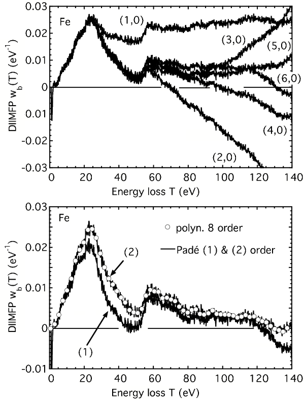
Figure 1: Illustration of the successive stages of the deconvolution of REELS spectra of Fe (measured at 1000 and 3400 eV) using an eighth order polynomial approximation (a.) and a second and first order Padé rational fraction approximation (Eqn. (8)) (b). The open circles in (b) are the result of the 8–th order polynomial expansion Eqn. (II), the solid curves labelled (1) and (2) are the first and second order Padé approximation, respectively. The curves shown represent the DIIMFP, the corresponding results for the DSEP are not shown for clarity, but behave in a similar way.

The W-algorithm has been succesfully applied to REELS data of a large number of materials Werner (2006c, 2005a); Zemek et al. (2006) and the dielectric function of several materials was succesfully extracted from the resulting DIIMFP and DSEP Werner (2006b, a). However, this approach may be improved upon in two respects: first of all, convergence of the series Eqn. (II) is relatively slow, implying that many terms need to be calculated; secondly, calculation of the higher order coefficients $u_{p,q}$ is tedious and time consuming. The moderate convergence behaviour of the W-algorithm is illustrated in Figure 1a that shows the various stages of the deconvolution. The first collision order $n$ indicated for the different curves implies that the second collision order has been taken into account up to $n-1$, so, for example, the curve labelled $(3,0)$ is a superposition of the $(1,0),(0,1),(1,1),(2,0),(2,1),(2,2)$ and $(3,0)$–th order cross-convolutions of the two experimental spectra. It is seen that more than 6 scattering orders need to be taken into account for the W-algorithm to converge over a loss range of about 100 eV.

The improvements addressed above can be effected following a suggestion by VicanekVicanek (1999) who pointed out that the TC-algorithm (for the univariate case) can in fact be regarded as a lowest order rational fraction expansion (a so–called Padé approximation) of the power series expansion of the spectrum. Extension of the concept of the Padé approximation to multivariate power series, such as Eqn. (9) is straightforward Cuyt (1999).

The simplified algorithm (designated by ”SW”–algorithm hereafter) is obtained (in Fourier space, indicated by the (”$\widetilde{~{}}$”)–symbol) by making the rational fraction ansatz :

$$\widetilde{w}=\frac{\sum\limits_{k=0}^{N}\sum\limits_{l=0}^{N}a_{k,l}\widetilde{y}^{k}_{1}\widetilde{y}^{l}_{2}}{\sum\limits_{k=0}^{N}\sum\limits_{l=0}^{N}b_{k,l}\widetilde{y}^{k}_{1}\widetilde{y}^{l}_{2}}$$ (8)

where $N$ is the order of the approximation and with $b_{0,0}=1$ and $a_{0,0}=0$. Note that the same formula holds for the quantities $w_{s}(T)$ and $w_{b}(T)$, only the expansion coefficients are different. Explicit expressions for the first order Padé coefficients as well as the system of linear equations determining the second order expansion coefficients, are given in the appendix. Multiplying Eqn. (8) with the denominator of the right hand side, and going back to real space one finds the deconvolution formula to be given by a Volterra integral equation of the second kind (being most harmless numerically):

$$w(T)=\sum\limits_{k=0}^{N}\sum\limits_{l=0}^{N}a_{k,l}Y_{k,l}(T)-\int\limits_{T^{\prime}=0}^{T}\sum\limits_{k=0}^{N}\sum\limits_{l=0}^{N}b_{k,l}Y_{k,l}(T-T^{\prime})w(T^{\prime})dT^{\prime}$$ (9)

where the quantity $Y_{k,l}(T)$ is the $(k,l)$-th order cross convolution of the two REELS spectra:

$$Y_{k,l}(T)=y_{1}^{(k)}(T-T^{\prime})\otimes y_{2}^{(l)}(T^{\prime})$$ (10)

Since $w(T=0)\equiv 0$ the integration on the right hand side of Eqn. (9) can always be carried out over the energy loss range for which the loss distribution is already known. For more details on the (trivial) numerical treatment of the Volterra integral equation of the second kind see, e.g., Ref. Press and Vetterling (1986).

The performance of the SW-algorithm is illustrated in Figure 1b, that shows the 8–th order polynomial expansion approximation (Eqn. (II)) as open circles. The solid curves labelled (1) and (2) are the first and second order Padé approximation results. It is seen that the latter converges as good as the polynomial expansion over the first $\sim$150 eV. Even the first order approximation leads to reasonable agreement. However, at least the second order mixed term (one surface and one bulk excitation) is important to attain quantitative agreement. The reason for the good performance of a rational fraction approximation compared to the polynomial expansion is clear: for a polynomial expansion, for any value of the variables a certain power in the series will always be the dominating term and may become arbitrarily large. For a rational fraction expansion, a large value of the dominant term in the enumerator can always be balanced by an appropriately chosen coefficient of the power in question in the denominator.

The second order SW-algorithm was applied REELS spectra of Ag, Al, Au, Be, Bi, C, Co, Fe, Ge, Mo, Mn, Ni, Pb, Pd, Pt, Si, Ta, Te, Ti, V, W and Zn) and was found to converge over the measured energy loss range of 140 eV. It can therefore be concluded that for an energy loss range of this order the second order SW-algorithm is sufficiently accurate. The main merit of the first order approximation is that the expansion coefficients can be given in a tractable analytical form (see the Appendix), providing detailed insight in the physical behaviour of the deconvolution. For example, it is seen in Eqn. (VIII) and (VIII) that the retrieved DIIMFP is completely independent of the value of the surface excitation parameter $a_{s}$ used for the deconvolution. On the other hand, the expansion coefficients for the surface loss probability are seen to scale linearly with $a_{s}$. This can be seen by substituting Eqn. (1) in Eqn. (VIII) and (VIII) and using Eqn. (4) and Eqn. (5). Thus, no information on surface excitations whatsoever is needed as input to the procedure (except the functional from of the dependence of the surface excitation probability on the energy and surface crossing direction, such as Eqn. (5)). Furthermore, as pointed out above, the value of the inelastic mean free path will mainly affect the absolute value of the partial intensities, $A_{n_{b}}$, while the reduced partial intensities $\alpha_{n_{b}}$ change negligibly when the IMFP is varied by up to 30%. Reasonably accurate knowledge of the shape and magnitude of the elastic scattering cross section is important, however, since the shape of the pathlength distribution depends on it. Near a deep minimum of the cross section this dependence may even be critical Werner (2005b), giving rise to qualitatively different sequences of partial intensities.

The higher order expansion coefficients also exhibit the scaling properties addressed above. Therefore, using a set of input parameters as discussed above, the normalized DIIMFP is correctly returned by the procedure in absolute units, while the correct shape of the DSEP is also obtained, but the absolute value of the DSEP scales with the value of $a_{s}$ used in the procedure.

Finally, it should be pointed out that by a suitable choice of the partial intensities (in particular letting $\beta_{n_{b}n_{s}}\rightarrow 0$, mimicking the use of a single REELS spectrum) Eqn. (9) reduces to the algorithms proposed by Vicanek Vicanek (1999) or Tougaard and Chorkendorff Tougaard and Chorkendorff (1987).

III Retrieval of Optical Data from the Single Scattering Distributions.

The procedure to extract the dielectric function of a solid from the DSEP and the DIIMFP has been outlined in Ref. Werner (2006b): The theoretical expressions for the DIIMFP and DSEP are fitted to the corresponding experimental results using a suitable model for the dielectric function. The differential inverse inelastic mean free path is related to the dielectric function $\varepsilon(\omega,q)$ of the solid via the well known formula Landau et al. (1984):

$$W_{b}(\omega)=\frac{1}{\pi E}\int\limits_{q_{-}}^{q_{+}}{\cal I}m\Big{\{}\frac{-1}{\varepsilon(\omega,q)}\Big{\}}\frac{dq}{q}.$$ (11)

For parabolic bands, the momentum transfer $q$ confined by $q_{-}$ and $q_{+}$ given by:

$$q_{\pm}=\sqrt{2E}\pm\sqrt{2(E-\omega)}.$$ (12)

Note that atomic units are used in this section. The differential inverse mean free path normalized to unity area is related to the unnormalized DIIMFP via $w_{b}(T)=\lambda_{i}W_{b}(T)$.

For the DSEP, the expression by Tung and coworkers Tung et al. (1994) is used:

$$W_{s}(\omega,\theta,E)=P_{s}^{+}(\omega,\theta,E)+P_{s}^{-}(\omega,\theta,E),$$ (13)

where the quantity $P_{s}^{\pm}(\omega,\theta,E)$ is defined as

$$P_{s}^{\pm}(\omega,\theta,E)=\frac{1}{\pi E\cos\theta}\int\limits_{q_{-}}^{q_{+}}\frac{|q_{s}^{\pm}|dq}{q^{3}}{\cal I}m\Big{[}\frac{(\varepsilon(\omega,q)-1)^{2}}{\varepsilon(\omega,q)(\varepsilon(\omega,q)+1)}\Big{]},$$ (14)

and

$$q_{s}^{\pm}=\Big{[}q^{2}-\big{(}\frac{\omega+q^{2}/2}{\sqrt{2E}}\big{)}^{2}\Big{]}^{1/2}\cos\theta\pm(\frac{\omega+q^{2}/2}{\sqrt{2E}})\sin\theta.$$ (15)

The normalized differential surface excitation probability is calculated via $w_{s}(T,\theta)=W_{s}(T,\theta)/\langle n_{s}(\theta,E)\rangle$.

The electromagnetic response of the solid is described in terms of the fit-parameters $f_{i},\omega_{i}$ and $\gamma_{i}$ using a model for the dielectric function in terms of a set of Drude-Lindhard oscillators for the evaluation of the theoretical expressions for the DIIMFP and DSEP Chen et al. (1993):

$$\varepsilon_{1}(\omega,q) = \varepsilon_{b}-\sum\limits_{i}\frac{f_{i}(\omega^{2}-\omega_{i}(q)^{2})}{(\omega^{2}-\omega_{i}(q)^{2})^{2}+\omega^{2}\gamma_{i}^{2}}$$

$$\varepsilon_{2}(\omega,q) = \sum\limits_{i}\frac{f_{i}\gamma_{i}\omega}{(\omega^{2}-\omega_{i}(q)^{2})^{2}+\omega^{2}\gamma_{i}^{2}},$$ (16)

where $\omega=T$ is the energy loss and $q$ is the momentum transfer. The static dielectric constant is given by $\varepsilon_{b}$, $f_{i}$ represents the oscillator strength, $\gamma_{i}$ the damping coefficient and $\omega_{i}$ is the energy of the $i$–th oscillator. Those values of the Drude–Lorentz parameters in the above equation that minimize the deviation between the experimental data and the theoretical expressions for the DIIMFP and DSEP are taken to parametrize the dielectric function. A quadratic dispersion $\omega_{i}(q)=\omega_{i}+q^{2}/2$ was used for the transition described by the $i$–th oscillator, except for those oscillators with an energy higher than the most loosely bound core electrons, that are assumed to be described by localized states without dispersion. Note that a dielectric function of the form Eqn. (III) implicitly satisfies the Kramers-Kronig dispersion relationships.

The (normalized) distributions $w_{b}(T)$ and $w_{s}(T)$ obtained from the experimental data are simultaneously fitted to the above theoretical expressions by minimizing the function:

$$X_{b}\chi^{2}_{DIIMFP}(p_{b},f_{i},\omega_{i},\gamma_{i})+X_{s}\chi^{2}_{DSEP}(p_{s},f_{i},\omega_{i},\gamma_{i}).$$ (17)

Here the function $\chi^{2}$ is the least squares difference between theory and experiment, defined in the usual way and $X_{b}$ and $X_{s}$ are weight factors chosen as $X_{b}=1.0$ and $X_{s}=0.1$, emphasizing the DIIMFP in the fitting procedure. The fit-parameters $p_{b}$ and $p_{s}$ are multiplicative scaling factors for the DIIMFP and the DSEP that compensate an eventual mismatch of the surface excitation parameter and IMFP used as input. Using the TPP-2M formula Tanuma et al. (1994) to estimate the IMFP, the value of $p_{b}$ deviated from unity by less than 5% for all cases studied, while the returned value of $p_{s}$ scales with the value of the surface excitation parameter $a_{s}$, exactly as anticipated in the previous section.

IV Experimental

The procedure used to acquire the experimental data has been described in detail before Werner et al. (2001a). REELS data were taken for polycrystalline Fe, Co and Ni surfaces in the energy range between 300 and 3400 eV for normal incidence and an off-normal emission angle of 60^∘, using a hemispherical analyzer operated in the constant-analyzer-energy mode giving a width of the elastic peak of 0.7 eV. Count rates in the elastic peaks were kept well below the saturation count rate of the channeltrons and a dead time correction was applied to the data. The sample was cleaned by means of sputtering with 3 keV Ar⁺ ions. Sample cleanliness was monitored with Auger electron spectroscopy.

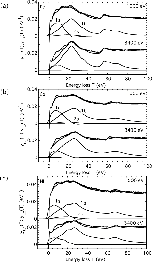
Figure 2: Experimental loss spectra for Fe, Co and Ni used in the present work (noisy curves). The thick solid curve is a fit of these data to Eqn. (6), using the retrieved optical data to describe the DIIMFP and DSEP. The thin solid curves labelled ”1s”, ”1b” and ”2s” represent the contribution of electrons having experienced one surface, one bulk and one and two surface excitations respectively.

For each material the optimum energy combination for the retrieval procedure of two loss spectra was determined by inspection of the partial intensities, choosing those energies for which on the one hand the determinant $\Delta$ in Eqn. (20) is reasonably large, while, on the other hand, those energies were avoided for which the scattering geometry corresponds to a deep minimum in the elastic cross section. For these cases it is more difficult to obtain the realistic shape of the pathlength distribution since the elastic cross sections are not accurately known for such scattering angles and the true electron optical detector solid angle also plays a significant role there. In Figure 2, the experimental spectra used in the present work are shown as noisy curves. For all selected energy combinations, the shape of the loss spectra is seen to be quite similar, but in all cases, a significant difference in the relative contribution of surface and bulk excitations is seen, as evidenced by the difference in spectral shape below $\sim$20 eV.

Removal of the elastic peak was achieved by fitting the elastic peak to a combination of a Gaussian and a Lorentzian peakshape. Subsequently, the fitted elastic peak was subtracted from the experimental data, they were divided by the area of the elastic peak, and the energy scale was converted to an energy-loss scale. Finally, the measured spectrum $S(T)$ [in counts per channel] was converted to experimental yield $y(T)$ [in reciprocal eV], corresponding to Equation (6), by division by the channel width $\Delta E$. Note that due to the dynamical range of a typical REELS spectrum measured with good energy resolution, a small misfit of the tail of the elastic peak can give erratic excursions in the loss spectra obtained in this way. This can be observed in Figure 2 for energy losses below $\sim$5 eV, where a negative excursion and a small shoulder right next to it are seen that are due to elimination of the elastic peak. The only way to cure this problem is to conduct the experiment with a better energy resolution, implying that the primary beam must be monochromatized.

V Results.

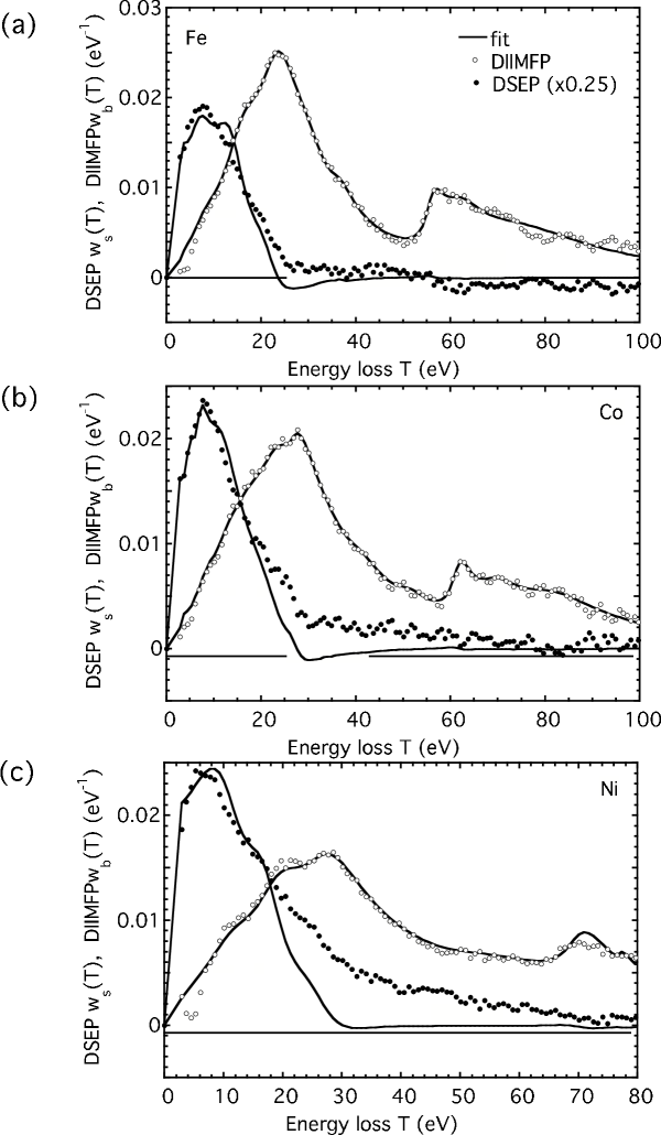
Figure 3: Normalized differential surface excitation probabililty (DSEP, $w_{s}(T)$) and normalized differential inverse inelastic mean free path (DIIMFP, $w_{b}(T)$) retrieved from the experimental data by means of Eqn. (9). The solid line is obtained by simultaneously fitting these data to theory for a set of Drude-Lorentz fit–parameters for the dielectric function, as described by Eqn. (III). The data for the surface excitation probability were scaled by a factor of 0.25 in order to facilitate comparison. (a) Fe; (b) Co; (c) Ni.

The DIIMFP and DSEP retrieved from the spectra displayed in Figure 2 with the second order SW–algorithm are presented in Figure 3 as open (DIIMFP) and filled circles (DSEP). The solid lines represent the best fit of the data to theory. It is seen that the DIIMFP can be perfectly fitted by the employed theory, while the corresponding DSEP agrees reasonably with the experimental data, but significant deviations are nonetheless observed. This is believed to be attributable to the simplifications concerning the depth dependence of the surface excitation process made in the employed theory for surface excitations Tung et al. (1994). The Drude–Lorentz parameters giving the best fit between experiment and theory are given in Table 1. The binding energy of the most loosely bound core electrons Werner et al. (2005) are also indicated there and are in good agreement with the energies of the ionization edges observed in Figure 3.

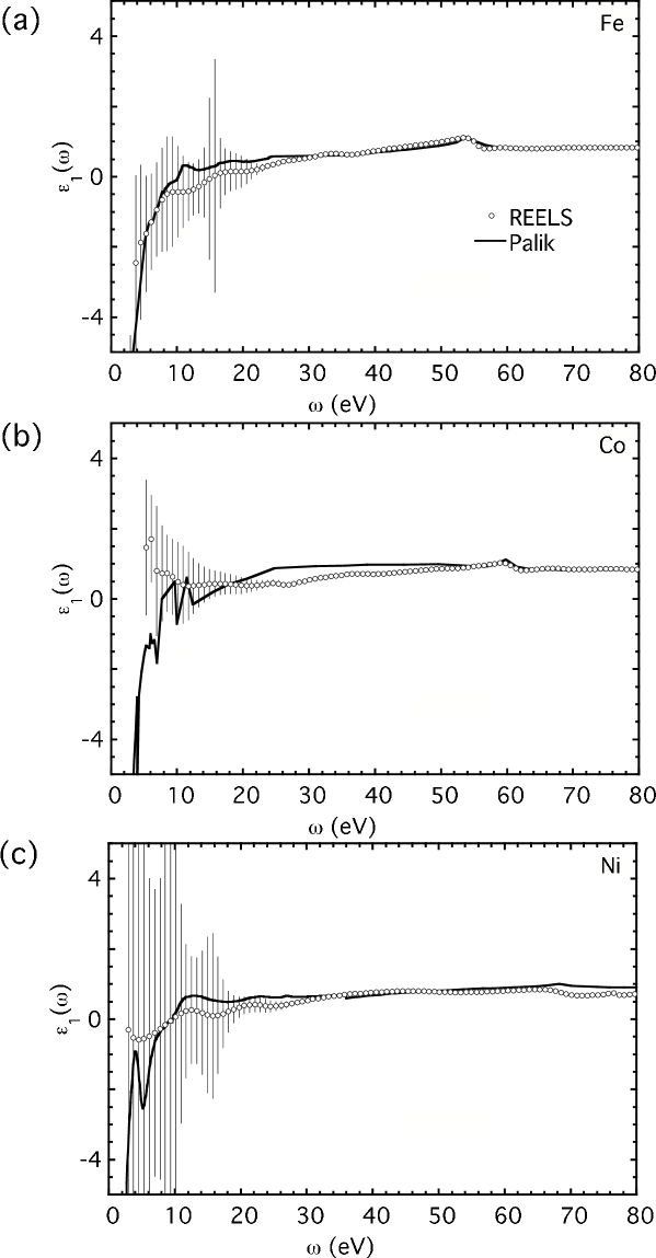
Figure 4: Real part of the dielectric function, $\varepsilon_{1}$, of Fe, Co and Ni retrieved from the REELS data (open circles) compared with Palik’s data Palik (1985, 1991) (solid curves). (a) Fe; (b) Co; (c) Ni.

A comparison of the real and imaginary part of the dielectric function derived from the REELS measurements with the data given in Palik’s book Palik (1985, 1991) is presented in Figure 4 and 5. Reasonable agreement between these two data sets is observed for all cases for energies $\gtrsim$5 eV. The error in the present data can become excessively large below 5 eV due to problems with the elimination of the elastic peak from the spectra. The error bars in these graphs are obtained Werner (2006a) by assuming that the retrieved DIIMFP predominantly determines $\varepsilon_{2}$ implying that the uncertainty in $\varepsilon_{2}$ is of the order of the uncertainty in the retrieved DIIMFP. The rules of error propagation are then used to estimate the uncertainty in $\varepsilon_{1}$. As can be seen the uncertainty in $\varepsilon_{1}$ is rather large below 20 eV. This is a fundamental characteristic of the derivation of optical data from absorption measurements, that mainly sample $\varepsilon_{2}$. Within the estimated uncertainty, the two data sets agree satisfactorily, both for the real as well as the imaginary part of $\varepsilon$.

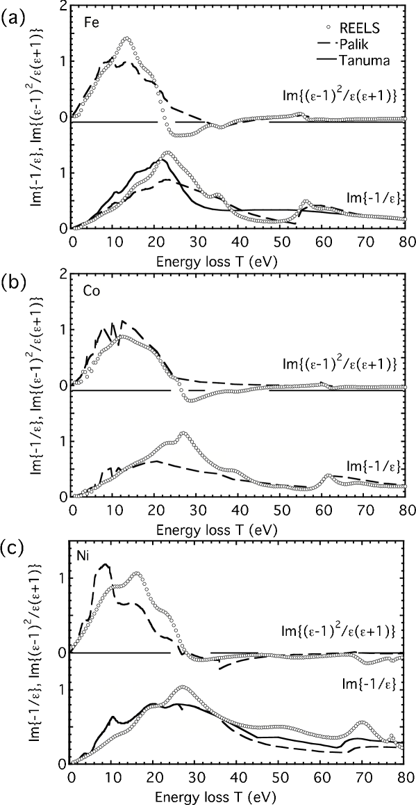
Figure 6: Volume and surface loss function of Fe, Co and Ni retrieved from REELS data (open circles) compared with Palik’s optical data (dashed curves). For the volume loss function of Fe and Ni, Tanuma’s data are also shown as solid curves. (a) Fe; (b) Co; (c) Ni.

The surface (upper panels) and bulk (lower panels) loss functions of Palik’s data and the present results are compared in Figure 6. For Fe and Ni, the data for the bulk loss function used by Tanuma, Powell and Penn Tanuma et al. (1994) is also shown for comparison. The general trend observed in these results is that for energies above $\sim$15 eV, the present data show more detailed structure in the loss function, while for lower energies, the earlier data seem to be more realistic. This is again attributable to the limited energy resolution used in the present study and the resulting problem with the elimination of the elastic peak.

To subject the present optical data to the usual sum–rule checks, the bulk loss function was extended above 80 eV by Palik’s data. The results for the perfect screening (or ”ps”) sum rule and the Thomas-Reiche-Kuhn (or ”f”) sum rule are compared with the corresponding results based on Palik’s and Tanuma’s loss functions in Table 2. The ps-sum rule seems to be the most important for the present study, since it emphasizes low energies, while the main contribution to the f-sum rule comes from the core electrons which are not fully included in the present measurements. Except for Ni, the ps-sum rule check for the REELS data is in better agreement with the expected value of 1.000 than for the two other sets of optical data. The f-sum rule shows deviations of the expected value of atomic electrons of the same order of magnitude for all data sets.

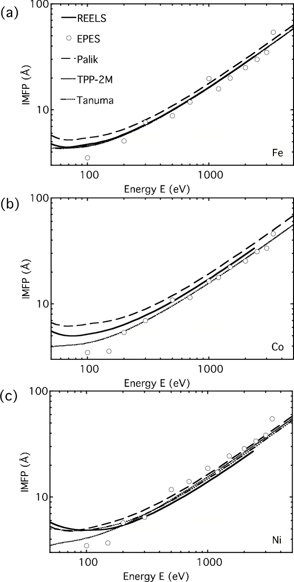
Figure 7: Inelastic mean free path of Fe, Co and Ni calculated from the optical data shown in Figure 6 (solid curves); Open circles represent experimental results measured with elastic peak electron spectroscopy (EPES) Werner et al. (2001b, a); Dashed curves represent calculations based on Palik’s optical data Palik (1985, 1991); The dotted curves represents the values predicted by the TPP-2M formula Tanuma et al. (1994); Chain dashed curves for Fe and Ni represent calculations based on Tanuma’s optical data Tanuma (Priv. Commun.) (a) Fe; (b) Co; (c) Ni.

Figure 7 shows the IMFP for the studied materials over the energy range between 50 and 5000 eV as thick solid line. For comparison, results using the other two sets of optical data are also shown as dashed (Palik) and chain dashed (Tanuma) curves. For the calculation of the IMFP of all three sets of optical data the software employed by the authors of Ref. Tanuma et al. (1994) was used Tanuma (Priv. Commun.). The results predicted by the TPP-2M-formula are indicated by the dotted line. The open circles represent the results of elastic peak electron spectroscopy (EPES) measurements reported earlier Werner et al. (2001a, b). The deviations of the IMFP values based on Palik’s data set and the present ones are most prominent for Co, which is caused by the lower value of Palik’s data for the loss function in the region between 20 and 50 eV. For Fe and Ni, the mutual agreement between the different IMFP values is satisfactory, except for energies below 100 eV, where the semiempirical TPP-2M formula predicts values for Co and Ni that are slightly lower than the other results. The EPES data differ from the other data sets in that the experimental elastic peak intensities are interpreted using only the elastic scattering cross section as input to the evaluation procedure Werner et al. (2001a); Powell and Jabłonski (1999), while the other calculations all are based on optical data and dielectric response theory. The two approaches are thus in a way fundamentally different. Nonetheless, the agreement between the EPES data and the IMFP values derived from the dielectric function is reasonable, at least within the experimental scatter of the EPES data.

As a final result, Figure 8 shows the surface excitation probability extracted from the REELS spectra as open circles. This quantity was determined by using the present optical data to calculate the normalized DIIMFP and DSEP and by fitting the experimental spectrum to theory via Eqn. (6) using $\langle n_{s}\rangle$ and the bulk partial intensities as fit parameters. Examples of such fits are shown in Figure 2 as thick solid lines. These fits are generally better than in previous work, where Palik’s optica data were used for the same purpose Werner et al. (2001c). The contribution of electrons that have experienced one bulk, one surface and two surface excitations is also indicated in these figures. The solid line in Figure 8 is a fit of the data for the surface excitation probability to Eqn. (5), the dotted line represents a fit to another functional from of the surface excitation probability that is commonly used Oswald (1992):

$$\langle n_{s}\rangle=\frac{1}{a^{*}_{s}\sqrt{E}\mu_{i}+1}+\frac{1}{a^{*}_{s}\sqrt{E}\mu_{o}+1},$$ (18)

the dashed and chain-dashed line are results by ChenChen (2002) and Kwei et al Kwei et al. (1998) respectively. The quality of these fits is also improved compared to earlier work, in that the values of the surface excitation probability $\langle n_{s}\rangle$ exhibit significantly less scatter than earlier Werner et al. (2001c). The resulting values of the surface excitation parameters $a_{s}$ and $a_{s}^{*}$ are given in Table 3. The present results for Fe are in excellent agreement with the value of $a_{s}=2.51$, reported by Chen (dashed line in Figure 8), while they are also in close agreement with the results quoted by Kwei and coworkers Kwei et al. (1998). The quality of the fit of the data to Eqn. (5) is generally slightly better than the fit to Eqn. (18), at least for Co and Ni, although it is still difficult on the basis of the present data to decide between the two functional forms for the SEP, Eqn. (5) and Eqn. (18). For this purpose, analysis of REELS experiments at higher energies would be required.

VI Summary and Conclusions.

An earlier proposed procedure Werner (2006c, 2005a) for the simultaneous deconvolution of two REELS spectra to provide the energy loss distribution in a single surface and volume electronic excitation is simplified using a Padé approximation and applied to experimental data of polycrystalline Fe, Co and Ni samples. It is shown that a second order rational fraction approximation converges better over an energy loss range of about 150 eV than an 8-th order polynomial expansion approximation, allowing one to conclude that the second order SW-algorithm can be safely used for practical purposes. Analysis of the expansion coefficients provide guidelines on the choice of the optimal experimental parameters to derive the DIIMFP and DSEP from REELS spectra and show, moreover, that no prior information on surface excitations is needed to perform the deconvolution. The retrieved DIIMFP and DSEP were fitted to the corresponding theoretical expressions giving the optical data of the studied solids in terms of a set of Drude-Lindhard parameters. Agreement between the resulting optical data as well as the IMFP derived from them with values based on optical data reported earlier is quite good, supporting the validity of the procedure. The values for the surface excitation probability retrieved from the data using the optical constants derived in this work are believed to be more reliable than the values reported earlier Werner et al. (2001c) and indicate that the energy and angular dependence of the surface excitation probability are described by Eqn. (5) rather than by Eqn. (18). The values for the surface excitation parameter are in reasonable agreement with theoretical values.

VII Acknowledgment

The author is grateful to Dr. S. Tanuma for making his optical data and his computer code for calculation of the IMFP available for the present comparison. Financial support of the present work by the Austrian Science Foundation FWF through Project No. P15938-N02 is gratefully acknowledged

VIII Appendix: First and Second Order Padé rational fraction expansion coefficients.

The explicit expressions for the first order bulk expansion coefficients in Eqn. (9) in terms of the partial intensities $\alpha_{n_{b}n_{s}}$ and $\beta_{n_{b}n_{s}}$ of two experimental REELS spectra are given by:

$$a^{b}_{00} = 0$$

$$a^{b}_{10} = {\beta_{01}}/\Delta$$

$$a^{b}_{01} = {-\alpha_{01}}/\Delta$$

$$b^{b}_{00} = 1$$

$$b^{b}_{10} = \frac{1}{\Delta^{2}}\Big{\{}\alpha_{20}\beta_{01}^{2}-\alpha_{11}\beta_{01}\beta_{10}+\alpha_{02}\beta_{10}^{2}+\alpha_{01}\beta_{10}\beta_{11}-\alpha_{01}\beta_{01}\beta_{20}-\frac{\alpha_{01}\beta_{02}\beta_{10}^{2}}{\beta_{01}}\Big{\}}$$

$$b^{b}_{01} = \frac{1}{\Delta^{2}}\Big{\{}\alpha_{10}^{2}\beta_{02}-\alpha_{01}\alpha_{10}\beta_{11}+\alpha_{01}^{2}\beta_{20}+\alpha_{10}\alpha_{11}\beta_{01}-\alpha_{01}\alpha_{20}\beta_{01}-\frac{\alpha_{02}\alpha_{10}^{2}\beta_{01}}{\alpha_{01}}\Big{\}}$$ (19)

where the determinant $\Delta$ is given by

$$\Delta={(\alpha_{10}\beta_{01}-\alpha_{01}\beta_{10})}$$ (20)

The surface expansion coefficients read:

$$a^{s}_{00} = 0$$

$$a^{s}_{10} = {-\beta_{10}}/\Delta$$

$$a^{s}_{01} = {\alpha_{10}}/\Delta$$

$$b^{s}_{00} = 1$$

$$b^{s}_{10} = \frac{1}{\Delta^{2}}\Big{\{}\alpha_{20}\beta_{01}^{2}-\alpha_{11}\beta_{01}\beta_{10}-\alpha_{10}\beta_{02}\beta_{10}+\alpha_{02}\beta_{10}^{2}+\alpha_{10}\beta_{01}\beta_{11}-\frac{\alpha_{10}\beta_{01}^{2}\beta_{20}}{\beta_{10}}\Big{\}}$$

$$b^{s}_{01} = \frac{1}{\Delta^{2}}\Big{\{}\alpha_{10}^{2}\beta_{02}-\alpha_{01}\alpha_{10}\beta_{11}-\alpha_{02}\alpha_{10}\beta_{10}+\alpha_{01}^{2}\beta_{20}+\alpha_{01}\alpha_{11}\beta_{10}-\frac{\alpha_{01}^{2}\alpha_{20}\beta_{10}}{\alpha_{10}}\Big{\}}$$ (21)

The expressions for the second order expansion coefficients are somewhat too lengthy to reproduce here. They can be easily calculated numerically though, by first establishing the polynomial expansion coefficients $u^{b}_{pq}$ and $u^{s}_{pq}$, as described in Refs.Werner (2006c, 2005a) up to third order ($p+q\leq 3$). The coefficients in the denominator of the rational fraction expansion are then found by solution of the homogeneous system of equations:

$$0 = b_{00}$$

$$0 = u_{30}+b_{10}u_{20}+b_{20}u_{10}$$

$$0 = u_{21}+b_{10}u_{11}+b_{01}u_{20}+b_{11}u_{10}+b_{20}u_{10}$$

$$0 = u_{12}+b_{10}u_{02}+b_{01}u_{11}+b_{11}u_{01}+b_{02}u_{10}$$

$$0 = u_{03}+b_{01}u_{02}+b_{02}u_{01}$$

$$0 = u_{22}+b_{10}u_{12}+b_{01}u_{21}+b_{11}u_{11}+b_{20}u_{02}+b_{02}u_{20}.$$ (22)

Finally, the enumerator coefficients are determined by the inhomogeneous system:

$$a_{00} = u_{00}=0$$

$$a_{10} = u_{10}$$

$$a_{01} = u_{01}$$

$$a_{11} = u_{11}+b_{10}u_{01}+b_{01}u_{10}$$

$$a_{20} = u_{20}+b_{10}u_{10}$$

$$a_{02} = u_{02}+b_{01}u_{01}.$$ (23)

	Fe			Co		Ni
	$E(3p_{1/2})$			$E(3p_{1/2})$		$E(3p_{3/2})$
	$52.7~{}eV$			$58.9~{}eV$		$66.2~{}eV$
Ai (eV${}^{2})$	$\gamma_{i}$ (eV)	$\omega_{i}$ (eV)	Ai (eV${}^{2})$	$\gamma_{i}$ (eV)	$\omega_{i}$ (eV)	Ai (eV${}^{2})$	$\gamma_{i}$ (eV)	$\omega_{i}$ (eV)
0.39	7.54	0.0	10.89	8.16	0.0	79.78	8.16	0.0
72.41	0.50	1.8	16.52	0.50	2.9	328.65	16.19	1.0
170.71	5.95	4.2	10.89	0.50	4.2	76.99	15.64	2.5
161.04	9.53	10.6	10.89	0.50	5.0	76.99	17.07	3.9
91.21	9.12	19.1	49.02	2.51	6.2	63.58	7.04	14.5
40.94	9.74	27.9	156.05	8.15	9.5	68.19	8.39	23.3
24.17	4.78	34.9	99.00	13.94	15.0	305.75	39.04	41.9
72.99	3.70	55.3	146.69	13.57	19.9	84.22	14.48	49.8
64.36	8.06	60.8	10.89	3.10	25.5	164.52	29.48	64.2
292.44	31.28	74.0	99.00	26.18	35.7	98.01	6.92	68.7
			15.39	5.62	38.8	7.59	1.35	76.9
			10.89	5.74	50.8
			60.53	3.92	60.9
			54.20	8.11	68.3

Table 1: Drude-Lindhard parameters for Fe, Co and Ni determined in the present work

	Fe	(Z=26)	Co	(Z=27)	Ni	(Z=28)
Ref.	f-sum	ps-sum	f-sum	ps-sum	f-sum	ps-sum
REELS	24.0	1.007	24.2	0.925	29.4	1.030
Palik	24.0	0.943	24.2	0.845	26.7	1.010
Tanuma	23.5	1.110	–	–	27.3	1.050

Table 2: Comparison of f- and ps-sum rule checks for different sets of optical data. The REELS data above 100 eV were extended to 30 keV using the data set of Palik

	$a_{s}$ (Eqn. (5))	$a_{s}^{*}$(Eqn. (18))
	$(eV^{1/2})$	$(eV^{-1/2})$
Fe	2.53	0.34
Co	2.79	0.30
Ni	2.84	0.30

Table 3: Surface excitation parameter $a_{s}$, according to Eqn. (5) and $a_{s}^{*}$, according to Eqn. (18) determined from the surface excitation probabilities shown in Figure 8

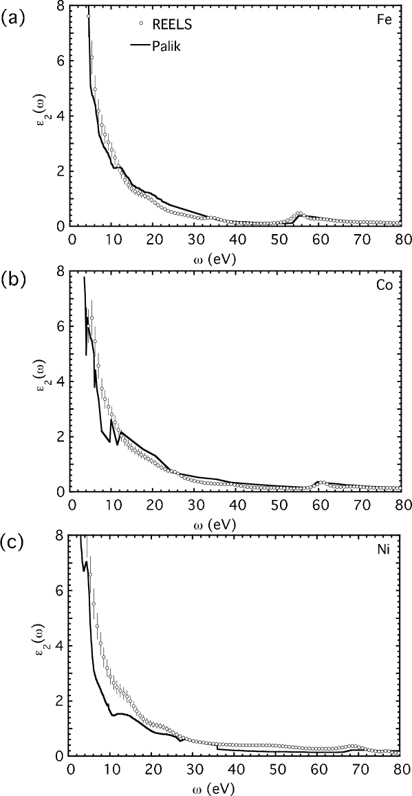
Figure 5: Imaginary part of the dielectric function, $\varepsilon_{1}$, of Fe, Co and Ni retrieved from the REELS data (open circles) compared with Palik’s data Palik (1985, 1991) (solid curves). (a) Fe; (b) Co; (c) Ni.

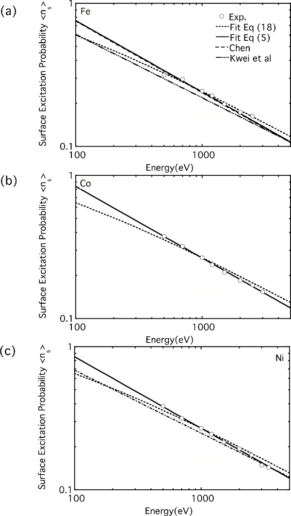
Figure 8: Surface excitation probability as a function of the energy for (a) Fe; (b) Co; and (c) Ni (open circles). The solid and dashed lines are fits of these data to Eqn. (5 and Eqn. (18) respectively). The dashed line shown for Fe is the theoretical dependence by Chen Chen (2002) which is almost impossible to distinguish from the present data. The chain-dashed curves for Fe and Ni represent the results by Kwei et al Kwei et al. (1998).

References

- Palik (1985) E. D. Palik, Handbook of optical constants of solids (Academic Press, New York, 1985).
- Palik (1991) E. D. Palik, Handbook of optical constants of solids II (Academic Press, New York, 1991).
- Henke et al. (1993) B. L. Henke, E. M. Gullikson, and J. C. Davis, Atomic Data and Nuclear Data Tables 54, 181 (1993).
- Chantler (1995) C. T. Chantler, J. Phys. Chem. Ref. Data 24, 71 (1995).
- Chantler (2000) C. T. Chantler, J. Phys. Chem. Ref. Data 29, 597 (2000).
- Schattschneider (1986) P. Schattschneider, Fundamentals of Inelastic Electron Scattering (Springer, New York, Vienna, 1986).
- Kohn (1999) W. Kohn, Rev. Mod. Phys. 71, 1253 (1999).
- Werner (2006a) W. S. M. Werner (2006a), submitted.
- Werner (2006b) W. S. M. Werner, Surf. Sci. (2006b).
- Blaha et al. (2002) P. Blaha, K. Schwarz, and G. K. H. Madsen, Comp.Phys.Commun. 71, 147 (2002).
- Tougaard and Chorkendorff (1987) S. Tougaard and I. Chorkendorff, Phys. Rev. B35, 6570 (1987).
- Werner (2006c) W. S. M. Werner, Phys. Rev. (2006c).
- Werner (2005a) W. S. M. Werner, Surf. Sci. 588, 26 (2005a).
- Vicanek (1999) M. Vicanek, Surf. Sci. 440, 1 (1999).
- Werner (2003) W. S. M. Werner, Surf. Sci. 526/3, L159 (2003).
- Werner (2005b) W. S. M. Werner, Surf. Interface Anal. 37, 846 (2005b).
- Jabłonski et al. (2004) A. Jabłonski, F. Salvat, and C. J. Powell, J. Phys. Chem. Ref. Data 33, 409 (2004).
- Tung et al. (1994) C. J. Tung, Y. F. Chen, C. M. Kwei, and T. L. Chou, Phys. Rev. B49, 16684 (1994).
- Zemek et al. (2006) J. Zemek, P. Jiricek, W. S. M. Werner, B. Lesiak, and A. Jablonski, Surf. Interface Anal. 38, 615 (2006).
- Cuyt (1999) A. Cuyt, J. Comput. Appl. Math. 105, 25 (1999).
- Press and Vetterling (1986) T. Press, Flannery and Vetterling, Numerical Recipes (Cambridge University Press, 1986).
- Landau et al. (1984) L. D. Landau, E. M. Lifshitz, and L. P. Pitaevski, Electrodynamics of Continuous Media (Pergamom Press, Oxford, New York, 1984), 2nd edition, Translated by J. B. Sykes, J. S. Bell and M. J. Kearsley.
- Chen et al. (1993) Y. F. Chen, C. M. Kwei, and C. J. Tung, Phys. Rev. B48, 4373 (1993).
- Tanuma et al. (1994) S. Tanuma, C. J. Powell, and D. R. Penn, Surf. Interface Anal. 21, 165 (1994).
- Werner et al. (2001a) W. S. M. Werner, C. Tomastik, T. Cabela, G. Richter, and H. Störi, J. Electron Spectrosc. Rel. Phen. 113, 127 (2001a).
- Werner et al. (2005) W. S. M. Werner, W. Smekal, and C. J. Powell, Simulation of Electron Spectra for Surface Analysis (National Institute for Standards and Technology (NIST), Gaithersburg (MD), US, 2005).
- Tanuma (Priv. Commun.) S. Tanuma (Priv. Commun.).
- Werner et al. (2001b) W. S. M. Werner, C. Tomastik, T. Cabela, G. Richter, and H. Störi, Surf. Sci. 470, L123 (2001b).
- Powell and Jabłonski (1999) C. J. Powell and A. Jabłonski, J Phys Chem Ref Data 28, 19 (1999).
- Oswald (1992) R. Oswald, Ph.D. thesis, Eberhard-Karls-Universität Tübingen (1992).
- Chen (2002) Y. F. Chen, Surf. Sci. 519, 115 (2002).
- Kwei et al. (1998) C. M. Kwei, C. Y. Wang, and C. J. Tung, Surf. Interface Anal. 26, 682 (1998).
- Werner et al. (2001c) W. S. M. Werner, W. Smekal, C. Tomastik, and H. Störi, Surf. Sci. 486, L461 (2001c).