Bose-Einstein condensates and EPR quantum non-locality

Abstract

The EPR argument points to the existence of additional variables that are necessary to complete standard quantum theory. It was dismissed by Bohr because it attributes physical reality to isolated microscopic systems, independently of the macroscopic measurement apparatus. Here, we transpose the EPR argument to macroscopic systems, assuming that they are in spatially extended Fock spin states and subject to spin measurements in remote regions of space. Bohr’s refutation of the EPR argument does not seem to apply in this case, since the difference of scale between the microscopic measured system and the macroscopic measuring apparatus can no longer be invoked.

In dilute atomic gases at very low temperatures, Bose-Einstein condensates are well described by a large population occupying a single-particle state; this corresponds, in the many particle Hilbert space, to a Fock state (or number state) with large number $N$. The situations we consider involve two such Fock states associated to two different internal states of the particles. The two internal states can conveniently be seen as the two eigenstates of the Oz component of a fictitious spin. We assume that the two condensates overlap in space and that successive measurements are made of the spins of single particles along arbitrary transverse directions (perpendicular to Oz).

In standard quantum mechanics, Fock states have no well defined relative phase: initially, no transverse spin polarization exists in the system. The theory predicts that it is only under the effect of quantum measurement that the states acquire a well defined relative phase, giving rise to a transverse polarization. This is similar to an EPR situation with pairs of individual spins (EPRB), where spins acquire a well defined spin direction under the effect of measurement - except that here the transverse polarization involves an arbitrary number of spins and may be macroscopic. We discuss some surprising features of the standard theory of measurement in quantum mechanics: strong effect of a small system onto an arbitrarily large system (amplification), spontaneous appearance of a macroscopic angular momentum in a region of space without interaction (non-locality at a macroscopic scale), reaction onto the measurement apparatus and angular momentum conservation (angular momentum version of the EPR argument).  Bohr’s denial of physical reality for microscopic systems does not apply here, since the measured system can be arbitrarily large. Since here we limit our study to very large number of particles, no Bell type violation of locality is obtained.

PACS 03.65. Ta and Ud ; 03.75.Gg

The famous Einstein-Podolsky-Rosen (EPR) argument EPR considers two correlated particles, located in two remote regions in space A and B, and focuses onto the “elements of reality” contained in these two regions. It starts from three ingredients: realism, locality, and the assumption that the predictions of quantum mechanics concerning measurements are correct; from these inputs it proves that, to provide a full description of physical reality, standard quantum mechanics must be completed with additional variables (often called “hidden variables” for historical reasons). The EPR argument was refuted by Bohr Bohr , who did not accept the notion of realism introduced by EPR; we give more details on his reply in § 1.  The purpose of the present article is to transpose the discussion to the macroscopic scale: we investigate situations that are similar to those considered by EPR but, instead of single particles, we study Bose-Einstein condensates made of many particles, which can be macroscopic. For dilute gases, these condensates can be represented as single quantum states populated with a large, but well defined, number of particles, in other words by Fock states (number states) with large $N$ (large, but well defined, population).

Several authors JH , WCW , CGNZ , CD , M-1 , M-2 , CCT , CH , PS , M3 , HB , DRB have studied the interference between two such condensates; since the phase of two Fock states is completely undefined according to standard quantum mechanics, the question is whether or not a well defined relative phase will be observed in the interference. These authors show that a well defined value of the relative phase can in fact emerge under the effect of successive quantum measurements. The value taken by this phase is random: it can be completely different form one realization of the experiment to the next. But, in a given realization, it becomes better and better defined while the measurements of the position of particles are accumulated. In other words, a perfectly clear interference pattern emerges from the measurements with a visible, but completely random and unpredictable, phase.

An interesting variant of this situation occurs if the two highly populated states correspond to two different internal states of the atoms SR , FL-1 , MKL . As usual, these two states can conveniently be seen as the two eigenstates of the $Oz$ component of a fictitious spin. One can then study for instance the situation shown schematically in fig. 1, where the two different internal states with high populations are initially trapped in two different sites, and then released to let them expand and overlap. Many other situations are also possible; we will discuss some of them in this article. In the overlap region, measurements of the spin component of particles along directions in the $xOy$ plane are sensitive to the relative phase of the two condensates. A free adjustable parameter for every measurement is the angle $\varphi$ which defines the direction of measurement in this plane; as discussed in MKL , this introduces more flexibility in choosing a strategy for optimum determination of the phase. Otherwise the situation is similar to that with spinless particles: initially the relative relative phase is completely undefined, and nothing can be said about its value. But, as long as the results of the measurements accumulate, the phase becomes better an better determined under the very effect of the quantum measurement process. This eventually creates a transverse spin polarization of the whole system, which can be macroscopic for large samples.

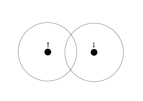
Figure 1: Two condensates, corresponding to two different internal spin states, expand and overlap in a region of space. In this region, particle spin measurements are performed in transverse directions (perpendicular to the spin directions of the two initial condensates).

We consider situations where two single particle states associated with different internal state of atoms overlap in space, and assume that each of these states has a large population. Transverse spin measurements are then performed in the region of overlap. This happens if two Bose-Einstein condensates are trapped in different sites, and then released to let them expand.

Usually, in the quantum theory of measurement, one emphasizes the role of a classical macroscopic pointer, the part of the measurement apparatus that directly provides the information to the human observer. Here we have a curious case where it is the measured system itself that spontaneously creates a pointer made of a macroscopic number of parallel spins. Moreover, for condensates that are extended in space, we will see that this process can create instantaneously parallel pointers in remote regions of space, a situation is obviously reminiscent of the EPR argument in its spin version given by Bohm (often called EPRB) B , BA . We study in this article how the EPR argument can be transposed to this case, and show that the argument becomes stronger, mostly because the measured systems themselves are now macroscopic. Bohr’s refutation, based on the denial of any physical reality for microscopic systems (cf. §1), then does not apply in the same way, if it still applies at all.

In § 1 we recall the main features of the EPR argument, which also gives us the opportunity to summarize Bohr’s reply and emphasize his fundamental distinction between microscopic observed systems and macroscopic measurement apparatuses. In § 2, we introduce the formalism and generalize the simple calculation of FL-1 , in particular to include the case where no particle is detected in the region of measurement. This provides us with the general expression of the joint probability for any sequence of spin measurements performed in the transverse direction, and any sequence of results. Then § 3 contains a discussion of the physics that is involved: amplification during quantum measurement, conservation of angular momentum and recoil effects of the measurements apparatus, quantum non-locality.

1 EPR argument and its refutation by Bohr

The EPR argument EPR FL-2 considers a physical system made of two correlated microscopic particles, assuming that they are located in two remote regions in space A and B where two physicists can perform arbitrary measurements on them. EPR specifically discuss situations where quantum mechanics predicts that the result of a first measurement performed in A is completely random, but nevertheless determines with complete certainty the result of another measurement performed in B. They introduce their “condition for the reality of a physical quantity” with the famous sentence: “if, without in any way disturbing a system, we can predict with certainty the value of a physical quantity, then there exists an element of physical reality corresponding to this physical quantity”. As a consequence, just after the measurement in A (but before the measurement in B), since the result of the second experiment is already certain, an element of reality corresponding to this certainty must exist in region B. But, according to locality, an element of reality in B can not have been created by the first measurement performed in region A, at an arbitrarily large distance; the element of reality necessarily existed even before any measurement. Since standard quantum theory does not contain anything like such a pre-existing element of reality, it is necessarily an incomplete theory; the state vector is not sufficient to describe a single realization of an experiment, but describes only a statistical ensemble of many realizations

Bohr, in his reply Bohr , does not criticize the EPR reasoning, but the assumptions on which it is based, which he considers as unphysical. He states that the criterion of physical reality proposed by EPR “contains an essential ambiguity when applied to quantum phenomena” and that “their argumentation does not seem to me to adequately meet the actual situation with which we are faced in atomic physics” (here, “atomic” is presumably equivalent to “microscopic” in modern language). His text has been discussed by many authors (for an historical review, see for instance MJ ), but still remains difficult to grasp in detail (see for instance Appendix I of Bell-1 ). Instead of concentrating his arguments on the precise situation considered by EPR, Bohr emphasizes in general the consistency of the mathematical formalism of quantum mechanics and the “impossibility of controlling the reaction of the object on the measuring instruments”. But, precisely, the main point of the EPR argument is to select a situation where these unavoidable perturbations do not exist! EPR locality implies that a measurement performed in regions A can create no perturbation on the elements of reality in region B.

Only the second part of Bohr’s article really deals with the EPR argument. After stating again that the words “without in any way disturbing the system” are ambiguous, he concedes that “there is of course in a case like that considered (by EPR) no question of a mechanical disturbance of the system under investigation during the last critical stage of the measuring procedure”. Nevertheless, for him what EPR have overlooked is that “there is essentially the question of an influence on the very conditions which define the precise types of predictions regarding the future behavior of the system” - the sentence is central but difficult; he probably means “an influence of the measurement performed in A on the conditions which define the predictions on the future behavior of the system in B, or maybe the whole system in both A and B”. He then states that these conditions are an essential element of any phenomenon to which the terms “physical reality” can be attached, and concludes that the EPR proof of incompleteness is non valid.

J.S. Bell summarizes the reply by writing Bell-1 that, in Bohr’s view “there is no reality below some classical macroscopic level”. For Bohr, it is incorrect to assign physical reality to one of the two particles, or even to the group of both particles; physical reality only has a meaning when macroscopic systems are involved, which here means the measurement apparatuses. He actually attaches physical reality only to the whole ensemble of the microscopic system and macroscopic measurement apparatuses, which extends over the two regions A and B of space, and not to subsystems. Then, the EPR reasoning, which focuses on B only, becomes incorrect. We remark in passing that Bohr’s refutation hinges on the microscopic character of the measured system, the two quantum particles.

2 Detecting the transverse direction of spins; calculation

We consider a system composed of particles having two internal states $\alpha$ and $\beta$, which can be seen as the eigenstates of the $Oz$ component of their spin with eigenvalues $+\hslash$/2 and $-\hslash$/2. The particles populate two quantum states, $\mid u_{a},\alpha>$ (orbital variables described by an orbital state $\mid u_{a}>$) and $\mid u_{b},\beta>$ (orbital state $\mid u_{b}>$). Initially, the quantum system is in a “double Fock state”, with $N_{a}$ particles populating the first single-particle-state and $N_{b}$ populating the other:

$$\mid\Phi>~{}=~{}\left[\left(a_{u_{a},\alpha}\right)^{\dagger}\right]^{N_{a}}\left[\left(a_{u_{b},\beta}\right)^{\dagger}\right]^{N_{b}}\mid\text{vac}.>$$ (1)

where $a_{u_{a},\alpha}$ and $a_{u_{b},\beta}$ are the destruction operators associated with the two single particle states, and $\mid$vac$.>$ is the vacuum state. With the notation of occupation numbers, the same initial state can also be written:

$$\mid\Phi>~{}=~{}\mid N_{a}:u_{a},\alpha~{};~{}N_{b}:u_{b},\beta~{}>$$ (2)

As in FL-1 , we note $\Psi_{\mu}(\mathbf{r})$, with $\mu=\alpha,\beta$, the field operators associated with internal states $\alpha$,$\beta$. The $\mathbf{r}$ dependent local density operator is then:

$$n(\mathbf{r})=~{}~{}\Psi_{\alpha}^{\dagger}(\mathbf{r})\Psi_{\alpha}(\mathbf{r})+\Psi_{\beta}^{\dagger}(\mathbf{r})\Psi_{\beta}(\mathbf{r})$$ (3)

while the three components of the local spin density are:

$$\begin{array}[c]{l}\sigma_{z}(\mathbf{r})=~{}\Psi_{\alpha}^{\dagger}(\mathbf{r})\Psi_{\alpha}(\mathbf{r})-\Psi_{\beta}^{\dagger}(\mathbf{r})\Psi_{\beta}(\mathbf{r})\\ \sigma_{x}(\mathbf{r})=~{}\Psi_{\alpha}^{\dagger}(\mathbf{r})\Psi_{\beta}(\mathbf{r})+\Psi_{\beta}^{\dagger}(\mathbf{r})\Psi_{\alpha}(\mathbf{r})\\ \sigma_{y}(\mathbf{r})=~{}i\left[\Psi_{\beta}^{\dagger}(\mathbf{r})\Psi_{\alpha}(\mathbf{r})-\Psi_{\alpha}^{\dagger}(\mathbf{r})\Psi_{\beta}(\mathbf{r})\right]\end{array}$$ (4)

The spin component in the direction of plane $xOy$ making an angle $\varphi$ with $Ox$ is:

$$\sigma_{\varphi}(\mathbf{r})=e^{-i\varphi}\Psi_{\alpha}^{\dagger}(\mathbf{r})\Psi_{\beta}(\mathbf{r})+~{}e^{i\varphi}\Psi_{\beta}^{\dagger}(\mathbf{r})\Psi_{\alpha}(\mathbf{r})$$ (5)

Suppose now that one measurement is made of the $\varphi$ component of the spin of particles within a small region of space $\Delta_{\mathbf{r}}$ centered around point $\mathbf{r}$. The corresponding operator is:

$$A(\mathbf{r},\varphi)=~{}\int_{\Delta_{\mathbf{r}}}d^{3}r^{{}^{\prime}}~{}\sigma_{\varphi}(\mathbf{r}^{{}^{\prime}})$$ (6)

If the volume $\Delta$ of domain $\Delta_{\mathbf{r}}$ is sufficiently small, the probability to find more than one particle in this volume is negligible, and $A(\mathbf{r},\varphi)$ has only three eigenvalues, $0$ and $\pm 1$. The eigenstates corresponding to the eigenvalue $\eta=0$ are all those where $\Delta_{\mathbf{r}}$ contains no particle; the eigenstates corresponding to the eigenvalues $\eta=\pm 1$ are those for which only one particle is within $\Delta_{\mathbf{r}}$, in a product state:

$$\mid\Delta_{\mathbf{r}},\eta>~{}=~{}\mid\Delta_{\mathbf{r}}>\otimes\frac{1}{\sqrt{2}}\left[e^{-i\varphi/2}\mid\alpha>+\eta e^{i\varphi/2}\mid\beta>\right]$$ (7)

where $\mid\Delta_{\mathbf{r}}>$ denotes a single particle orbital state with wave function given by the characteristic function of domain $\Delta_{\mathbf{r}}$ (equal to $1$ in this domain, $0$ elsewhere). In the limit where the volume $\Delta$ tends to $0$, one can ignore states with more than one particle in $\Delta_{\mathbf{r}}$, and the $N$ particle states in question provide a quasi-complete basis. The projector onto eigenvalue $0$ is:

$$P_{\eta=0}(\mathbf{r})=~{}1-\int_{\Delta_{\mathbf{r}}}d^{3}r^{{}^{\prime}}~{}n(\mathbf{r}^{{}^{\prime}})=\int_{\Delta_{\mathbf{r}}}d^{3}r^{{}^{\prime}}~{}\left[\frac{1}{\Delta}-n(\mathbf{r}^{{}^{\prime}})\right]$$ (8)

On the other hand, the projectors for eigenvalues $\eta=\pm 1$ are:

$$P_{\eta=\pm 1}(\mathbf{r,\varphi})=\,\frac{1}{2}\int_{\Delta_{\mathbf{r}}}d^{3}r~{}\left[n(\mathbf{r})+\eta\sigma_{\varphi}(\mathbf{r})\right]$$ (9)

We now consider a series of $K$ measurements, the first of a spin along direction $\varphi_{1}$ in volume $\Delta_{\mathbf{r}_{1}}$, the second of a spin along direction $\varphi_{2}$ in volume $\Delta_{\mathbf{r}_{2}}$, etc., corresponding to the sequence of operators:

$$A(\mathbf{r}_{1},\varphi_{1})\text{ \ ; \ }~{}A(\mathbf{r}_{2},\varphi_{2})\text{ \ ; \ }~{}A(\mathbf{r}_{3},\varphi_{3})~{};...~{};~{}A(\mathbf{r}_{K},\varphi_{K})$$ (10)

As in FL-1 , we assume assume that all $\mathbf{r}$’s are different and that the regions of measurement $\Delta_{\mathbf{r}_{1}}$, $\Delta_{\mathbf{r}_{2}}$, …, $\Delta_{\mathbf{r}_{K}}$ do not overlap, so that all these operators commute; in addition, and as already mentioned, we assume that the sequence of measurements is sufficiently brief to ignore any intrinsic evolution of the system other than the effect of the measurements themselves. Under these conditions, the probability of any sequence of results:

$$\eta_{1}=0,\pm 1\text{\ \ ; \ }~{}\eta_{2}=0,\pm 1\text{ \ ; \ }...~{}~{}~{}~{}\eta_{K}=0,\pm 1$$ (11)

is simply given by the average value in state $\mid\Phi>$ of the product of projectors:

$$<\Phi\mid P_{\eta_{1}}(\mathbf{r}_{1}\mathbf{,\varphi}_{1})\times P_{\eta_{2}}(\mathbf{r}_{2}\mathbf{,\varphi}_{2})\times....P_{\eta_{K}}(\mathbf{r}_{K}\mathbf{,\varphi}_{K})\mid\Phi>$$ (12)

When the projectors are replaced by their expressions (8) and (9), with (5), we obtain the product of several terms, each containing various products of field operators. In each term, because of the commutation of the measurements, we can push all $\Psi_{\alpha,\beta}^{\dagger}(\mathbf{r})$’s to the left, all $\Psi_{\alpha,\beta}(\mathbf{r})$’s to the right. It is then useful to expand the field operators onto the annihilation operators for single-particle-states $\mid u_{a},\alpha>$ and $\mid u_{b},\beta>$:

$$\Psi_{\alpha}(\mathbf{r})~{}=~{}u_{a}(\mathbf{r})\times a_{u_{a},\alpha}+....~{}~{}\text{;}~{}~{}~{}\Psi_{\beta}(\mathbf{r})~{}=~{}u_{b}(\mathbf{r})\times a_{b,\beta}+....~{}$$ (13)

where the terms $+....~{}$ symbolize sums over other orbital states that, together with $u_{a}(\mathbf{r})$, or $u_{b}(\mathbf{r})$, complete a basis in the orbital space state of a single particle. Since the destruction operators give zero when they act on states that have zero population, it is easy to see that all these additional terms simply disappear. Each term now contains between the bra $<\Phi\mid$ and the ket $\mid\Phi>$ a sequence of  creation operators, $\left(a_{u_{a},\alpha}\right)^{{\dagger}}$ or $\left(a_{u_{b},\beta}\right)^{{\dagger}}$, followed by another sequence of destruction operators, $\left(a_{u_{a},\alpha}\right)$ or $\left(a_{u_{b},\beta}\right)$. If each state, $u_{a},\alpha$ or $u_{b},\beta$, does not appear exactly the same number of times in the sequence of creation operators and the sequence of destruction operators, one obtains the product of two orthogonal kets, which is zero. If they appear exactly the same number of times, every creation and destruction operator introduces a factor $\sqrt{\left(N_{a,b}-q\right)}$, where $q$ depends on the term considered, but remains smaller than the number of measurements $K$. We assume that:

$$K\ll N_{a}~{},~{}N_{b}$$ (14)

which allows us to approximate, as in FL-1 , all factors $\sqrt{\left(N_{a,b}-q\right)}$ by $\sqrt{N_{a,b}}$.

At this point, all operators of $\ \Psi_{\alpha,\beta}^{\dagger}(\mathbf{r})$ are simply replaced by $\sqrt{N_{a,b}}u_{a,b}^{\ast}(\mathbf{r})$, all $\Psi_{\alpha,\beta}(\mathbf{r})$ by the complex conjugate, but we still have to take into account the necessity for particle number conservation in each sequence. This can be done by using the mathematical identity:

$$\int_{0}^{2\pi}\frac{d\Lambda}{2\pi}~{}e^{in\Lambda}~{}=~{}\delta_{n,0}$$ (15)

(where $n$ is an integer): if we multiply each $\Psi_{\alpha}(\mathbf{r})$ (or $\sqrt{N_{a}}u_{a}(\mathbf{r})$) by $e^{i\Lambda}$, and each $\Psi_{\alpha}^{\dagger}(\mathbf{r})$ (or $\sqrt{N_{a}}u_{a}^{\ast}(\mathbf{r})$) by $e^{-i\Lambda}$, and then integrate $\Lambda$ over $2\pi$, we express the necessary condition and automatically ensure particle number conservation.

We remark that neither $n(\mathbf{r})$ nor $P_{\eta=0}(\mathbf{r})$ introduce exponentials of $\Lambda$, since they always contain matched pairs of creation and destruction operators; exponentials only appear in $\sigma_{\varphi}(\mathbf{r})$ that is in the projectors $P_{\eta}(\mathbf{r,}$$\varphi$$)$ when $\eta=\pm 1$. We assume that volume $\Delta$ is sufficiently small to neglect the variations of the orbital wave functions over all $\Delta_{\mathbf{r}}$’s. The probability of the sequence of results (11) is then proportional to :

$$\begin{array}[c]{l}{\displaystyle\prod\limits_{i}}\left[1-\Delta\left(N_{a}\left|u_{a}(\mathbf{r}_{i})\right|^{2}+N_{b}\left|u_{b}(\mathbf{r}_{i})\right|^{2}\right)\right]\times\\ \times\int_{0}^{2\pi}\frac{d\Lambda}{2\pi}{\displaystyle\prod\limits_{j}}\left\{\Delta\left[N_{a}\left|u_{a}(\mathbf{r}_{j})\right|^{2}+N_{b}\left|u_{b}(\mathbf{r}_{j})\right|^{2}+\eta_{j}\sqrt{N_{a}N_{b}}\left(e^{i\left(\Lambda-\varphi_{j}\right)}u_{a}(\mathbf{r}_{j})u_{b}^{\ast}(\mathbf{r}_{j})+\text{c.c.}\right)\right]\right\}\end{array}$$ (16)

where c.c. means complex conjugate. In this expression, the first line corresponds to the contribution of all results $\eta=0$ (no particle found in the volumes of detection) and has no $\Lambda$ (or $\varphi$) dependence; the second line corresponds to all positive detections of spins of particles. It is convenient to introduce the relative phase of the two wave functions by:

$$\xi(\mathbf{r})=\arg\left[u_{a}(\mathbf{r})/u_{b}(\mathbf{r})\right]$$ (17)

so that the brackets in the second line become:

$$\left[N_{a}\left|u_{a}(\mathbf{r}_{j})\right|^{2}+N_{b}\left|u_{b}(\mathbf{r}_{j})\right|^{2}+2\eta_{j}\sqrt{N_{a}N_{b}}_{a}\left|u_{a}(\mathbf{r}_{j})\right|\left|u_{b}(\mathbf{r}_{j})\right|\cos\left(\Lambda+\xi(\mathbf{r}_{j})-\varphi_{j}\right)\right]$$ (18)

The contrast of the interference pattern is maximal at points $\mathbf{r}_{j}$ where $\sqrt{N_{a}}\left|u_{a}(\mathbf{r}_{j})\right|=\sqrt{N_{b}}\left|u_{b}(\mathbf{r}_{j})\right|$, i.e. where the two boson fields have the same intensity.

These are is the result onto which our discussion below will be based; for a generalization to spin measurements that are not necessarily in the $xOy$ plane, see the appendix of MKL .

3 Physical discussion

3.1 Role of the $\Lambda$ integral

Suppose that we consider a sequence where only one spin is detected; the product over $j$ in (16) then contains only one bracket, summed over $\Lambda$ between $0$ and $2\pi$. The contribution of each value of $\Lambda$ gives nothing but the probability of the two results, $\eta_{j}=\pm 1$, for a spin $1/2$ that is described by a density matrix $\rho$ given by:

$$\rho\propto\left(\begin{array}[c]{ll}N_{a}\left|u_{a}(\mathbf{r}_{1})\right|^{2}&\sqrt{N_{a}N_{b}}u_{a}^{\ast}(\mathbf{r}_{j})u_{b}(\mathbf{r}_{1})e^{-i\Lambda}\\ \sqrt{N_{a}N_{b}}u_{a}(\mathbf{r}_{1})u_{b}^{\ast}(\mathbf{r}_{1})e^{i\Lambda}&N_{b}\left|u_{b}(\mathbf{r}_{1})\right|^{2}\end{array}\right)$$ (19)

This is easily checked by calculating the trace of the product of $\rho$ by the projector:

$$\left[1+\eta\left(e^{-i\varphi}\sigma_{+}+e^{i\varphi}\sigma_{-}\right)\right]/2$$ (20)

The $Oz$ component of the spin before measurement is then proportional to $N_{a}\left|u_{a}(\mathbf{r}_{1})\right|^{2}-N_{b}\left|u_{b}(\mathbf{r}_{1})\right|^{2}$, its transverse component proportional to $2\sqrt{N_{a}N_{b}}_{a}\left|u_{a}(\mathbf{r}_{1})\right|\left|u_{b}(\mathbf{r}_{1})\right|$, with an azimuthal direction specified by angle $\Lambda-\xi(\mathbf{r}_{1})$. Now, since $\Lambda$ is summed between $0$ and $2\pi$, the off diagonal elements disappear from (19), meaning that this azimuthal direction is initially completely random; the spin loses its transverse orientation and keeps only its $Oz$ component. This is natural since we are starting from Fock states with completely undetermined relative phase. Therefore, for the first transverse measurement the two results $\pm 1$ always have the same probability, and the adjustable parameter $\varphi_{1}$ plays no role.

Now consider a sequence with two measurements and two results $\eta_{1,2}=\pm 1$. In (16), the $\Lambda$ integral then introduces correlations. The result of the first measurement provides an information on the probabilities of the results of the second: this information is contained in a $\Lambda$ distribution that is given by (18), with $\eta_{j}$ replaced by the result $\pm 1$ of the first measurement, and $\mathbf{r}_{j}$ replaced by the point $\mathbf{r}_{1}$ at which this measurement was made. The information is still not very precise, since the width of the $\Lambda$ distribution is of the order of $\pi$; but, for instance, if the first result was $+1$ and if the two angles of measurements $\varphi_{1}$ and $\varphi_{2}$ are close or even equal, there is more chance to find again $+1$ than $-1$ for the result of the second measurement.

When more and more spin measurements are obtained, the $\Lambda$ distribution becomes narrower and narrower, meaning that more and more information on the value of $\Lambda$ is accumulated. Standard quantum mechanics considers that $\Lambda$ has no physical existence at the beginning of the series of measurements, and that its determination is just the result of a series of random perturbations of the system introduced by the measurements. Nevertheless, (16) shows that all observations are totally compatible with the idea of a pre-existing value of $\Lambda$, which is perfectly well defined but unknown, remains constant, and is only revealed (instead of being created) by the measurements. For a more detailed discussion of the evolution of the $\Lambda$ distribution, and of the optimum strategy concerning the choice of the angles of measurement $\varphi_{j}$ to better determine $\Lambda$, see ref. MKL .

It is interesting to find a situation where an additional (hidden) variable $\Lambda$ emerges so naturally from a standard calculation in quantum mechanics. It appears mathematically as a way to express the conservation of number of particles. In other words, the role of the additional variable is, by integration, to ensure the conservation of the conjugate variable. This contrasts with usual theories with additional variables, where they are introduced more or less arbitrarily, the only constraint being that the statistical average over the new variables reproduces the predictions of standard quantum mechanics.

3.2 Small and big condensates; amplification during measurement

In our calculation, we have made no special assumption concerning the orbital wave functions $u_{a}(\mathbf{r})$ and $u_{b}(\mathbf{r})$ associated with the two highly populated single particle quantum states; they can overlap much or little in space, and in many ways. We will consider situations where their configuration leads to the discussion of interesting physical effects. For simplicity, from now on we assume that the two wave functions have the same phase at every point of space $\mathbf{r}$, so that $\xi(\mathbf{r})$ vanishes. This simplification occurs if the two states correspond to stationary states trapped in a real potential, as often the case in experiments with Bose-Einstein condensates; it is convenient, but not essential.

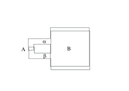
Figure 2: Two different spin states ($\alpha=+$ and $\beta=-$) are associated with two orbital wave functions that overlap mostly in a large region B, but also have “fingers” that overlap in a much smaller region A. The two states are macroscopically populated. Under the influence of a few measurements of the spin of particles performed in region A, a macroscopic transverse spin polarization appears in region B.

As a first example, we consider two states such as those represented schematically in figure 2. The states are mostly located in a region of space B where they strongly overlap, but also have “fingers” that overlap in another small region of space A, where the spin measurements are actually performed. We assume that A is not too small, and contains an average number of spins (100 for instance) that remains sufficient to perform several measurements and determine the relative phase of the two Fock states with reasonable accuracy. On the other hand, the number of spins in region B may be arbitrarily large, of the order of the Avogadro number for instance.

In this situation, our preceding calculation applies and predicts that the measurement of the spins in A will immediately create a spontaneous polarization in B that is parallel to the random polarization obtained in A. In other words, standard quantum mechanics predicts a giant amplification effect, where the measurement performed on a few microscopic particles induces a transverse polarization in a macroscopic assembly of spins. In itself, the idea is not too surprising, even in classical mechanics: one could see the assembly of spins in B as a metastable system, ready to be sensitive to the tiny perturbation of a microscopic system in A. In this perspective, the perturbations created by the measurement in A would propagate towards B and trigger its evolution towards a given spin direction. But this is not the context in which we have obtained the prediction: we have not assumed any evolution of the state vector of the system between one measurement and the next. In fact, what standard quantum mechanics describes here is not something that propagates along the state and has a physical mechanism (such as, for instance, the propagation of Bogolubov phonons in the condensates); it is just “something with no time duration” that is a mere consequence of the postulate of quantum measurement (wave packet reduction).

Leggett and Sols LS , L discuss a similar situation in the context of two large superconductors, which acquire a spontaneous phase by the creation of a Josephson current between them, which in turn is measured by a tiny compass needle in order to obtain its phase. Here again we have a small system determining the state of a much larger system, without any physical mechanism. These authors comment the situation in the following terms: “can it really be that by placing, let us say, a minuscule compass needle next to the system, with a weak light beam to read off its position, we can force the system to realize a definite macroscopic value of the current? Common sense rebels against this conclusion, and we believe that in this case common sense is right”. They then proceed to explain that the problem may arise because we are trying to apply to macroscopic objects quantum postulates that were designed 80 years ago for the measurements of microscopic objects, because other measurements were not conceivable then. In other words, we are trying to use present standard quantum mechanics beyond its range of validity. They conclude that what is needed in a new quantum measurement theory.

What is interesting to note, as we have already mentioned in the introduction, is that here we have a case where the measured system itself creates a macroscopic pointer, made of a large assembly of parallel spins, that directly “shows” the direction of the spins resulting from the measurements. Usually, in the theory of quantum measurement, this pointer is the last part of the measuring apparatus, not something that interacts directly with the measured system itself, or even less is part of it.

3.3 EPR non locality with Fock states

Now suppose that the two condensates have the shape sketched in figure 3, extending over a large distances, and overlapping only in two remote regions of space A and B. Again, the number of particles in both regions is arbitrary, and in particular can be macroscopic in B. We have a situation that is similar to the usual EPR situation: measurements performed in A can determine the direction of spins in both regions A and B. If we rephrase the EPR argument to adapt it to this case, we just have to replace the words “before the measurement in A” by “before the series of measurements in A”, but all the rest of the reasoning remains exactly the same: since the elements of reality in B can not appear under the effect of what is done at an arbitrary distance in region A, these elements of reality must exist even before the measurements performed in A. Since the initial double Fock state of quantum mechanics does not contain any information on the direction of spins in B, this theory is incomplete.

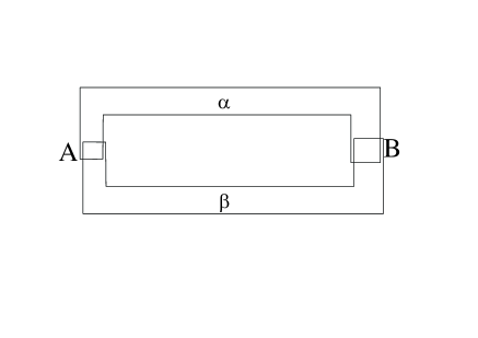
Figure 3: Two highly populated Fock states associated with opposite spin direction ($\alpha=+$ and $\beta=-$) overlap in two remote regions A and B of space. A series of transverse spin measurements in A triggers the appearance of a well defined transverse orientation in A, and also that of a parallel macroscopic transverse orientation in B (quantum non locality). This corresponds to an angular momentum that seems to appear in B from nothing, with no interaction at all.

What is new here is that the EPR elements of reality in B correspond to a system that is macroscopic. One can no longer invoke its microscopic character to deprive the system contained in B of any physical reality! The system can even be at our scale, correspond to a macroscopic magnetization that can be directly observable with a hand compass; is it then still possible to state that it has no intrinsic physical reality? When the EPR argument is transposed to the macroscopic world, it is clear that Bohr’s refutation does no longer apply in the form written in his article; it has to be at least modified in some way.

Another curiosity, in standard quantum mechanics, is that it predicts the appearance of a macroscopic angular momentum in region B without any interaction. This seems to violate angular momentum conservation. Where does this momentum come from? Usually, when a spin is measured and found in some state, one considers that the angular momentum is taken as a recoil by the measurement apparatus. When the measured system is microscopic and the apparatus macroscopic, the transfer of angular momentum is totally negligible for the latter, so that there is no hope to check this idea; but, at least, one can use the idea as a theoretical possibility. Here, the situation is more delicate: what is the origin of the angular momentum that appears in B during measurement? Could it be that the apparatus in A, because the system in A is entangled with a macroscopic system in B, takes a macroscopic recoil, even if it measures a few spins only? A little analysis shows that this is impossible without introducing the possibility for superluminal communication: the recoil in A would allow to obtain information on B (if the states have been dephased locally for instance). So, it can not be the measurement apparatus in A that takes the angular momentum recoil corresponding to B. Then, if we believe that angular momentum can not appear in a region of space without interactions, even during operations that are considered as “measurements” in standard quantum mechanics, this leads us to an ”angular momentum EPR proof”: we are forced to conclude that the transverse polarization of the spins in B already existed before any measurement started. Since this is not contained in the double Fock state, standard quantum mechanics is incomplete.

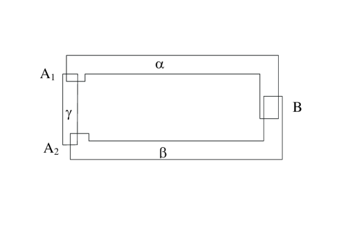
Figure 4: In a variant of the situation shown in Fig. 3, measurements are performed in region A, at points A₁ and A₂, of the relative phase between a small local condensate (in internal state $\gamma$) and two extended condensates (respectively in internal states $\alpha$ and $\beta$). By transitivity, this determines the relative phase of the large condensates, resulting by interference in a transverse spin polarization in region B. Even if the measurements with the local A condensate do not involve angular momentum (assumed to have no matrix elements between the overlapping states), this operation can create a macroscopic angular momentum in region B.

We can make the argument even more convincing by using the scheme sketched in figure 4. We now assume that the two condensates in internal states $\alpha$ and $\beta$ overlap in B but not in A, where they both overlap both with the same third condensate in a third internal state $\gamma$. We furthermore assume that angular momentum has matrix elements between $\alpha$ and $\beta$, but not between $a$ and $\gamma$ and between $\beta$ and $\gamma$ (for instance, the parity of $\gamma$ may be the opposite of that of the two other internal states): the transverse measurements in A correspond to some observable that has appropriate matrix elements and parity, electric dipole for instance. We know (see for instance FL-1 ) that phase determination in Fock states is transitive: fixing the phase between $a$ and $\gamma$ on the one hand, between $\beta$ and $\gamma$ on the other, will determine the relative phase of $\alpha$ and $\beta$. Under these conditions, in standard quantum mechanics, the macroscopic angular momentum that appears in B can be a consequence of measurements in A of physical quantities that have nothing to to with angular momentum, so that the measurement apparatuses have no reason to take any angular momentum recoil at all. Still, they create a large angular momentum in B. Again, if we do not accept the idea of angular momentum appearing from nothing, we must follow EPR and accept that the angular momentum was there from the beginning, even if we had no way to predict its direction.

4 Possible objections

In this text, we have discussed thought experiments, not attempted to propose feasible experiments. We have just assumed that the states that are necessary for the discussion can be produced, and that they are sufficiently robust to undergo a series of measurements, with no other perturbation than the measurements themselves; this may require that the sequence of measurements be sufficiently fast. Of course, one could always object that these double Fock states are fundamentally not physical, for instance because some selection rule forbids them. This would be in contradiction with the generally accepted postulate that all quantum states belonging to the space of states (Hilbert space) of any physical system are accessible. If this postulate is true, there should be no fundamental reason preventing the preparation of a double Fock state, even for a system containing many particles.

A second objection could be that these states may exist but be so fragile that, in practice, it will always be impossible to do experiments with them. In the context of second order phase transitions and spontaneous symmetry breaking, Anderson A-1 , A-2 , A-3 has introduced the notion of spontaneous phase symmetry breaking for superfluid Helium 4 and superconductors. According to this idea, coupled superfluid systems at thermal equilibrium are not in Fock states: as soon as they become superfluid by crossing the second order transition, some unavoidable small perturbation always manages to transform the simple juxtaposition of the two Fock states into a single coherent Fock state containing all the $N_{a}+N_{b}$ particles, for which the two quantum states have a well defined relative phase. This assumption is for example implicit in the work of Siggia and Ruckenstein SR , where the two condensates are considered as having a well defined phase from the beginning.

In our discussion, we have assumed neither the existence of a second order phase transition nor even thermal equilibrium, just the availability of the large initial double Fock state. Is there any general mechanism that favours coherent states over double Fock states? Decoherence may actually inroduce this preference. As in ref. PS , we can introduce the so called coherent “phase states” by:

$$\mid\phi,N>~{}=\frac{1}{\left(2^{N}N!\right)^{1/2}}~{}\left[e^{i\phi/2}\left(a_{u_{a},\alpha}\right)^{\dagger}+e^{-i\phi/2}\left(a_{u_{b},\beta}\right)^{\dagger}\right]^{N}\mid\text{vac}.>$$ (21)

in terms of which the ket $\mid\Phi>$ of (2) can be written:

$$\mid N_{a}:u_{a},\alpha~{};~{}N_{b}:u_{b},\beta~{}>\propto\int_{0}^{2\pi}d\phi~{}e^{i\left(N_{b}-N_{a}\right)\phi}\mid\phi,N>$$ (22)

If $M$ is large, the phase state (21) have a macroscopic transverse orientation in an azimuthal direction defined by $\phi$; this orientation is likely to couple to the external environment, as most macroscopic variable do. For instance, if the spin of particles is associated with a magnetic moment, the different phase states create different macroscopic magnetic fields that will affect at least some microscopic particles of the environment, transferring them into states that are practically orthogonal for different values of $\phi$. In other words, the basis of phase states is the “preferred basis” for the system coupled to its environment. As a consequence, the coherent superposition (22) spontaneously transforms into a superposition where each component, defined by a very small $\phi$ domain, is correlated with a different state of the environment. The correlation quickly propagates further and further into the environment, without any limit as long as the Schrödinger equation is obeyed (this is the famous Schrödinger cat paradox). As a result, the observation of interference effects between different $\phi$ values becomes more and more difficult, in practice impossible. In terms of the the trace of the density operator over the environment, the coherent superposition (22) decays rapidly into an incoherent mixture of different $\phi$ states. For a general discussion of the observability of macroscopically distinct quantum states, see for instance ref. AJL .

Decoherence is unavoidable, but does not really affect our conclusions. It just means that, in the standard interpretation, when the measurements are performed in region A and determine the transverse polarization, they fix at the same time the spin directions in B as well as the state of the local environment. The real issue is not coherence, or the coupling to the environment; it is the emergence of a single macroscopic result, which is considered as an objective fact and a result of the observation in the standard interpretation (but of course not in the Everett interpretation). In the end, decoherence is not an essential issue in our discussion.

A third objection might be size limitations: are there inherent limits to the size of highly populated Fock states and Bose-Einstein condensates? Is there any reason why large sizes should make them extremely sensitive to small perturbations? One could think for instance of thermal fluctuations that may introduce phase fluctuations and put some temperature dependent limit on the size of the coherent system. Other possible mechanisms, such as inhomogeneities of external potentials, might break the condensate into several independent condensates, etc. Generally speaking, we know that ideal condensed gases are extremely sensitive to small perturbations, but fortunately also that repulsive interactions between the atoms tend to stabilize condensed systems. They do not only introduce a finite compressibility of the condensate, but also tend to stabilize the macroscopic occupation of a single quantum state PN . This should increase the robustness of large systems occupying a unique single Fock state, even if extended in space.

Experimentally, Bose-Einstein condensates in dilute gases at very low temperatures provide systems that are very close to being in a highly populated Fock state. Nevertheless, until now experiments have been performed with gas samples that are about the size of a tenth of a millimeter; one can therefore not exclude that new phenomena and unexpected perturbations will appear when much larger condensates are created. In any case, even if the non-local effects that we have discussed are limited to a range of a tenth of a millimeter (or any other macroscopic length), they remain non-local effects on which a perfectly valid EPR type argument can be built!

5 Conclusion

We can summarize the essence of this article by saying that, in some quantum situations where macroscopic systems populate Fock states with well defined populations, the EPR argument becomes significantly stronger than in the historical example with two microscopic particles. The argument speaks eloquently if favour of a pre-existing relative phase of the two states - alternatively, if one prefers, of an interpretation where the phase remains completely undetermined even after the measurements (Everett interpretation) - but certainly not in favour of the orthodox point of view where the phase appears during the measurements. If we stick to this orthodox view, surprising non-local effects appear in the macroscopic world. These effects can be expressed in various ways, including considerations on macroscopic angular momentum conservation, but not in terms of violations of Bell type inequalities (this is because the form of the $\Lambda$ integral in (16), with positive terms inside it, automatically ensures that the Bell inequalities are satisfied). In any case, Bohr’s denial of physical reality of the measured system alone becomes much more difficult to accept when this system is macroscopic. Of course, no one can predict what Bohr would have replied to an argument involving macroscopic spin assemblies, and whether or not he would have maintained his position concerning the emergence of a single macroscopic result during the interaction of the measured system with the measurement apparatuses.

Another conclusion is that quantum mechanics is indeed incomplete, not necessarily in the exact sense meant by EPR, but in terms of the postulates related to the measurement: they do not really specify what is the reaction of the measured system on the measurement apparatus (“recoil effect”). Ignoring this reaction was of course completely natural at the time when quantum mechanics was invented: only quantum measurements of microscopic systems were conceivable at that time, so that these effects were totally negligible. But now this is no longer true, so that we need a more complete theory for quantum measurement on a macroscopic system “in which all the assumptions about relative energy and time scales, etc.. are made explicit and if necessary revised” LS . Bose-Eintein condensates in gases seem to be good candidates to explore this question theoretically and experimentally.

Acknowledgments

The author is grateful to W. Mullin, A. Leggett, C. Cohen-Tannoudji and J. Dalibard for useful discussions and comments.

References

- [1] A. Einstein, B. Podolsky and N. Rosen, “Can quantum-mechanical description of physical reality be considered complete?”, Phys. Rev. 47, 777-780 (1935).
- [2] N. Bohr, “Can quantum-mechanical description of physical reality be considered complete?”, Phys. Rev. 48, 696-702 (1935).
- [3] J. Javanainen and Sun Mi Ho, “Quantum phase of a Bose-Einste in condensate with an arbitrary number of atoms”, Phys. Rev. Lett. 76, 161-164 (1996).
- [4] T. Wong, M.J. Collett and D.F. Walls, “Interference of two Bose-Einstein condensates with collisions”, Phys. Rev. A 54, R3718-3721 (1996)
- [5] J.I. Cirac, C.W. Gardiner, M. Naraschewski and P. Zoller, “Continuous observation of interference fringes from Bose condensates”, Phys. Rev. A 54, R3714-3717 (1996).
- [6] Y. Castin and J. Dalibard, “Relative phase of two Bose-Einstein condensates”, Phys. Rev. A 55, 4330-4337 (1997)
- [7] K. Mølmer, “Optical coherence: a convenient fiction”, Phys. Rev. A 55, 3195-3203 (1997).
- [8] K. Mølmer, “Quantum entanglement and classical behaviour”, J. Mod. Opt. 44, 1937-1956 (1997)
- [9] C. Cohen-Tannoudji, Collège de France 1999-2000 lectures, chap. V et VI “Emergence d’une phase relative sous l’effet des processus de détection” http://www.phys.ens.fr/cours/college-de-france/.
- [10] Y. Castin and C. Herzog, “Bose-Einstein condensates in symmetry breaking states”, C.R. Acad. Sci. série IV, 2, 419-443 (2001).
- [11] C.J. Pethick and H. Smith, “Bose-Einstein condensates in dilute gases”, Cambridge University Press (2002); see chap. 13.
- [12] K. Mølmer, “Macroscopic quantum-state reduction: uniting Bose-Einstein condensates by interference measurements”, Phys. Rev. A 65, 021607 (2002).
- [13] P. Horak and S.M. Barnett, “Creation of coherence in Bose-Einstein condensates by atom detection”, J. Phys. B 32, 3421-3436 (1999).
- [14] J. Dunningham, A. Rau and K. Burnett “From pedigree cats to fluffy-bunnies”, Science 307, 872-875 (2005).
- [15] E. Siggia and A. Ruckenstein, “Bose condensation in spin-aligned atomic hydrogen”, Phys. Rev. Lett. 44, 1423-1426 (1980).
- [16] F. Laloë, “The hidden phase of Fock states; quantum non-local effects”, Europ. Phys. J. section D, 33, 87-97 (2005).
- [17] W.J. Mullin, R. Krotkov and F. Laloë, Phys. Rev. A74, 023610 (2006).
- [18] D. Bohm, “Quantum theory”, Prentice Hall (1951).
- [19] D. Bohm and Y. Aharonov, “Discussion of experimental proof for the paradox of Einstein, Rosen, and Podolsky”, Phys. Rev. 108, 1070 (1957).
- [20] F. Laloë, “Do we really understand quantum mechanics”, Am. J. Phys. 69, 655-701 (2001) or (more recent version) quant-ph/0209123.
- [21] M. Jammer, “The philosophy of quantum mechanics”, Wiley (1974), chapter 6.
- [22] J.S. Bell, “Bertlmann’s socks and the nature of reality”, J. Physique Colloque C2, supplément au no 3, 42, 41-61 (1981). This article is reprinted in Bell-2
- [23] J.S. Bell, “Speakable and unspeakable in quantum mechanics”, Cambridge University Press (1987).
- [24] M.H. Wheeler, K.M. Mertes, J.D. Erwin and D.S. Hall “Spontaneous macroscopic spin polarization in independent spinor Bose-Einstein condensates”, Phys. Rev. Lett. 89, 090402 (2002).
- [25] A.J. Leggett and F. Sols, “On the concept fo spontaneously broken gauge symmetry in condensed matter physics”, Foundations of physics 21, 353 (1991).
- [26] A.J. Leggett, “Broken gauge symmetry in a Bose condensate”, in “Bose-Einstein condensation”, A. Griffin, D.W. Snoke and S. Stringari eds., Cambridge University Press (1995); see in particular pp. 458-459.
- [27] P.W. Anderson, “Considerations on the flow of superfluid helium”, Rev. Mod. Phys. 38, 298-310 (1966).
- [28] P.W. Anderson, “Basic notions in condensed matter physics”, Benjamin-Cummins (1984).
- [29] P.W. Anderson, “Measurement in quantum theory and the problem of complex systems”, in “The Lesson of quantum theory” ed. by J. de Boer, E. Dal and O. Ulfbeck, Elsevier (1986); see section 3.
- [30] A.J. Leggett, “Testing the limits of quantum mechanics: motivation, state of play, prospects”, J. Phys. Condens. Matter 14, R415-R451 (2002).
- [31] P. Nozières, “Some comments on Bose-Einstein condensation”, in “Bose-Einstein condensation”; edited by A. Griffin, D.W. Snoke and S. Stringari, Cambridge University Press (1995).
- [32] W.E. Lamb and A. Nordsieck, “On the Einstein condensation phenomenon”, Phys. Rev. 59, 677 (1941).