Scaling of fluctuations in a colloidal glass

Abstract

We report experimental measurements of particle dynamics in a colloidal glass in order to understand the dynamical heterogeneities associated with the cooperative motion of the particles in the glassy regime. We study the local and global fluctuation of correlation and response functions in an aging colloidal glass. The observables display universal scaling behavior following a modified power-law, with a plateau dominating the less heterogeneous short-time regime and a power-law tail dominating the highly heterogeneous long-time regime.

I Introduction

Mostly due to the enormous practical importance of glassy systems there has been a vast literature describing different theoretical frameworks for glasses, yet without a common theory applicable to the diverse range of systems undergoing a glass transition. Increasing the volume fraction of a colloidal system slows down the Brownian dynamics of its constitutive particles, implying a limiting density, $\phi_{g}$, above which the system can no longer be equilibrated with its bath Pusey . Hence, the thermal system falls out of equilibrium on the time scale of the experiment and thus undergoes a glass transition Cugliandolo . Even above $\phi_{g}$ the particles continue to relax, but the nature of the relaxation is very different to that in equilibrium. This phenomenon of a structural slow evolution beyond the glassy state is known as “aging” Struik . The system is no longer stationary and the relaxation time is found to increase with the age of the system, $t_{w}$, as measured from the time of sample preparation.

This picture applies not only to structural glasses such as colloids, silica and polymer melts, but also to spin-glasses, ferromagnetic coarsening, elastic manifolds in quenched disorder and jammed matter such as grains and emulsions Cugliandolo ; Kurchan_prl ; Bouchaud .

In order to investigate the dynamical properties of the aging regime we consider the evolution of the correlation function $C(t,t_{w})$ and integrated response to external fields $\chi(t,t_{w})$. These quantities are separated into a stationary (short time) and an aging part (long time): $C(t,t_{w})=C_{\rm st}(t-t_{w})+C_{\rm ag}(t,t_{w})$ and $\chi(t,t_{w})=\chi_{\rm st}(t-t_{w})+\chi_{\rm ag}(t,t_{w})$, where we have included the explicit dependence on $t_{w}$ in the aging part, and $t$ is the observation time.

We use a simple system undergoing a glass transition: a colloidal glass of micrometer size particles, where the interactions between particles can be approximated as hard core potentials Pusey ; Kegel ; Weeks_sci . The system is index matched to allow the visualization of tracer particles in the microscope Weeks_sci . Owing to the simplicity of the system, we are able to follow the trajectories of magnetic tracers embedded in the colloidal sample and use this information to understand the scaling of the local and global fluctuations of the correlation functions.

II Experimental setup

Our experiments use a colloidal suspension consisting of a mixture of poly-(methylmethacrylate) (PMMA) sterically stabilized colloidal particles (radius $a_{p}=1.5\ \mu m$, density $\rho_{p}=1.19\ g/cm^{3}$, polydispersity $\sim 14\%$) plus a small fraction of superparamagnetic beads (radius $a_{m}=1.6\ \mu m$ and density $\rho_{m}=1.3\ g/cm^{3}$, from Dynal Biotech Inc.) as the tracers

The colloidal suspension is immersed in a solution containing $76\%$ weight fraction of cyclohexylbromide and $24\%$ cis-decalin which are chosen for their density and index of refraction matching capabilities Weeks_sci . For such a system the glass transition occurs at $\phi_{g}\approx 0.57-0.58$ Pusey ; Kegel ; Weeks_sci . In our experiments we consider two samples at different densities and determine the glassy phase for the samples that display aging. The main results are obtained for sample A just above the glass transition $\phi_{\rm A}=0.58\pm 0.01$. We also consider a denser sample B with $\phi_{\rm B}=0.60\pm 0.01$, although this sample is so deep in the glassy phase that we are not able to study the slow relaxation of the system and the dependence of the waiting time within the time scales of our experiments.

We use a magnetic force as the external perturbation to generate two-dimensional motion of the tracers Song on a microscope stage following a simplified design of magnetic_stage . Video microscopy and computerized image analysis are used to locate the tracers in each image. We calculate the response and correlation functions in the x-y plane.

The experimental set up is shown in Fig. 1a and Fig. 1b. We use a Zeiss microscope with a 50$\times$ objective of numerical aperture 0.5 and a working distance of 5mm. We work with a field of view $194\mu m\times 155\mu m$ by using a digital camera with the resolution of 1288 pixels $\times$ 1032 pixels. We locate the center of each bead position with sub-pixel accuracy, by using image analysis. For the condensed samples A and B, we use the low frame rate $1/3$ frame/sec, while for the dilute sample C, we record the images at $1$ frame/sec. The long working distance of the objective is necessary to allow the pole of the magnet to reach a position near the sample. An example of the images of the tracers obtained in sample A is shown in Fig. 1c where we can see the black magnetic tracers embedded in the background of nearly transparent PMMA particles. An example of the trajectory in the x-y plane of a tracer diffusing without magnetic field is shown in Fig. 1d. We note that this particular tracer moves away from two cages in a time of the order of $4$ hours.

The magnetic field is produced by one coil made of 1200 turns of copper wire. We arrange the pole of the coil perpendicular to the vertical optical axis, and generate a field with no vertical component. Thus, the tracers move in the x-y plane with a slight vertical motion which is generated by a density mismatch between the tracers and the background PMMA particles. This vertical motion is very small at the high volume fraction of interest here, and therefore we calculate all the observables in the x-y plane.

The magnetic force is calibrated for a given coil current by replacing the suspension with a mixture of $50:50$ water-glycerol solution with a few magnetic tracers. The distance between the top of the magnetic pole and the vertical optical axis is always fixed, which means that the magnetic force at the local plane depends only on the coil current. At a given current, we determine the velocity of the magnetic tracers at the focal point and calculate the magnetic force from Stokes’s law, $F=6\pi\eta a_{m}v$, where $\eta$ is the viscosity of the water-glycerol solution, $a_{m}$ is the tracer radius, and $v$ is the observed velocity of the tracer. The uncertainty in the obtained force comes from: (a) the uncertainty in the coil current which is $1\%$, (b) the beads, which are not completely monodisperse in their magnetic properties, causes a $10\%$ uncertainty Weeks_force , and (c) the magnetic field is slowly decaying in the field of view, causing a $4\%$ uncertainty.

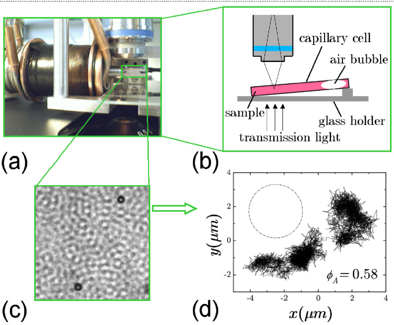
Figure 1: (a) Picture of the experimental setup. (b) Schematic illustration of the setup. (c) Detail of an image of tracer in sample A. (d) Trajectory of a tracer in sample A showing the cage dynamics over 4 hours. The circle represents the size of the tracer particle, $3.2\mu m$.

In order to investigate the dynamical properties of the aging regime, we first consider the autocorrelation function as the mean square displacement (MSD) averaged over 82 tracer particles, $C(t,t_{w})\equiv\langle\Delta x^{2}(t,t_{w})\rangle/2=\langle[x(t_{w}+\Delta t,t_{w})-x(t_{w},t_{w})]^{2}\rangle/2$, at a given observation time, $t=t_{w}+\Delta t$, after the sample has been aging for $t_{w}$ as measured from the end of the stirring process. Then, we measure the integrated response function (by adding the external magnetic force, $F$) given by the average position of the tracers, $\chi(t,t_{w})\equiv\langle x(t_{w}+\Delta t,t_{w})-x(t_{w},t_{w})\rangle/F$.

III Sample Preparation at $t_{w}=0$

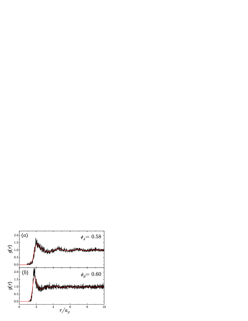
Figure 2: Pair-distribution functions of (a) sample A and (b) sample B.

It is important to correctly determine the initial time of each measurement to reproduce the subsequent particle dynamics. We initialize the system by stirring the sample for two hours with an air bubble inside the sample (see Fig. 1b) to homogenize the whole system and break up any pre-existing crystalline regions. Then we place the sample on the magnetic stage and take images to obtain the trajectories of the tracers that appear in the field of view. The initial times $t=t_{w}=0$ are defined at the end of the stirring. After measuring all the tracers appearing in the field of view, a new stirring is applied, the waiting time is reset to zero, and the measurements are repeated for a new set of tracers. We have analyzed the pair-distribution function, $g(r)$, and two-time intensity autocorrelation function, $g_{2}(t_{w},t_{w}+\Delta t)$, in order to test our rejuvenation technique.

First, Fig. 2 plots the pair-distribution functions of sample A and sample B right after the stirring procedure. We calculate the pair-distribution functions by reconstructing the packings from 3D confocal microscopy images of size $60\mu m{\times}60\mu m{\times}15\mu m$. We find that the samples do not show obvious crystallized region by directly looking either at the pair-distribution function or the images taken from confocal microscopy.

For these measurements we use a Leica confocal microscope. The PMMA particles are fluorescently dyed so that they are ready to be observed by confocal microscopy. We load the samples sealed in a glass cell on the confocal microscope stage and use a Leica HCX PL APO 63x, 1.40 numerical aperture, oil immersion lens for 3D particle visualization in order to calculate the volume fraction and the pair-distribution function.

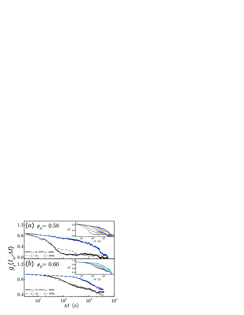
Figure 3: Two-time intensity autocorrelation function, $g_{2}(t_{w}+\Delta t,t_{w})$, of (a) sample A and (b) sample B. The solid black and navy curves correspond to $t_{w}=0$s and $t_{w}=4000$s, respectively. The dash gray and light blue curves correspond to the measurements after the second stirring with ${t_{w}}^{{}^{\prime}}=0$s and ${t_{w}}^{{}^{\prime}}=4000$s, respectively. The fact that the curves at $t_{w}=0$s and ${t_{w}}^{{}^{\prime}}=0$s coincide indicates that sample has been fully rejuvenated to its initial state. The inset is the same plot as the main figure for different $t_{w}$ ranging from 0s (solid black) to 4000s (solid navy).

Second, we analyze $g_{2}(t_{w}+\Delta t,t_{w})$ and show that the sample has been rejuvenated by the stirring process. We plot $g_{2}(t_{w}+\Delta t,t_{w})$ for 3 situations: (a) after the first stirring process ($t_{w}=0$), (b) after the sample has aged for a long time ($t_{w}=4000s$), (c) we then apply the stirring again and immediately plot the autocorrelation function for the new initial time (${t_{w}}^{{}^{\prime}}=0$). The plot show the lack of correlation for the two individual measurements $t_{w}=0$ and ${t_{w}}^{{}^{\prime}}=0$, thus demonstrating that the sample has been rejuvenated. Technically, we record the temporal image sequence of sample A and sample B, and study the aging by calculating two images’ correlation defined as:

$$g_{2}(t_{w},t_{w}+\Delta t)=\frac{\langle I(t_{w})I(t_{w}+\Delta t)\rangle}{\langle I(t_{w})^{2}\rangle},$$ (1)

where $I$ is the average gray-scale intensity of a small box (20 pixels $\times$ 20 pixels, PMMA particles’ diameter is roughly equal to 20 pixels), and $I(t_{w})$ and $I(t)$ come from the images at different times $t_{w}$ and $t$, respectively. We cut one image (1288 pixels $\times$ 1032 pixels) into many boxes, and calculate the correlation of two boxes located at the same position in the two images. The average $\langle...\rangle$ is taken over all the boxes in one image. Fig. 3 plots the correlation function, $g_{2}(t_{w},t_{w}+\Delta t)$, of sample A and sample B, which shows aging behavior (see the inset). Fig. 3 shows how $g_{2}(t_{w},t_{w}+\Delta t)$ calculated after two stirring processes at $t_{w}=0$ and ${t_{w}}^{{}^{\prime}}=0$ coincide, indicating that the sample can be fully rejuvenated to its initial state by our stirring technique.

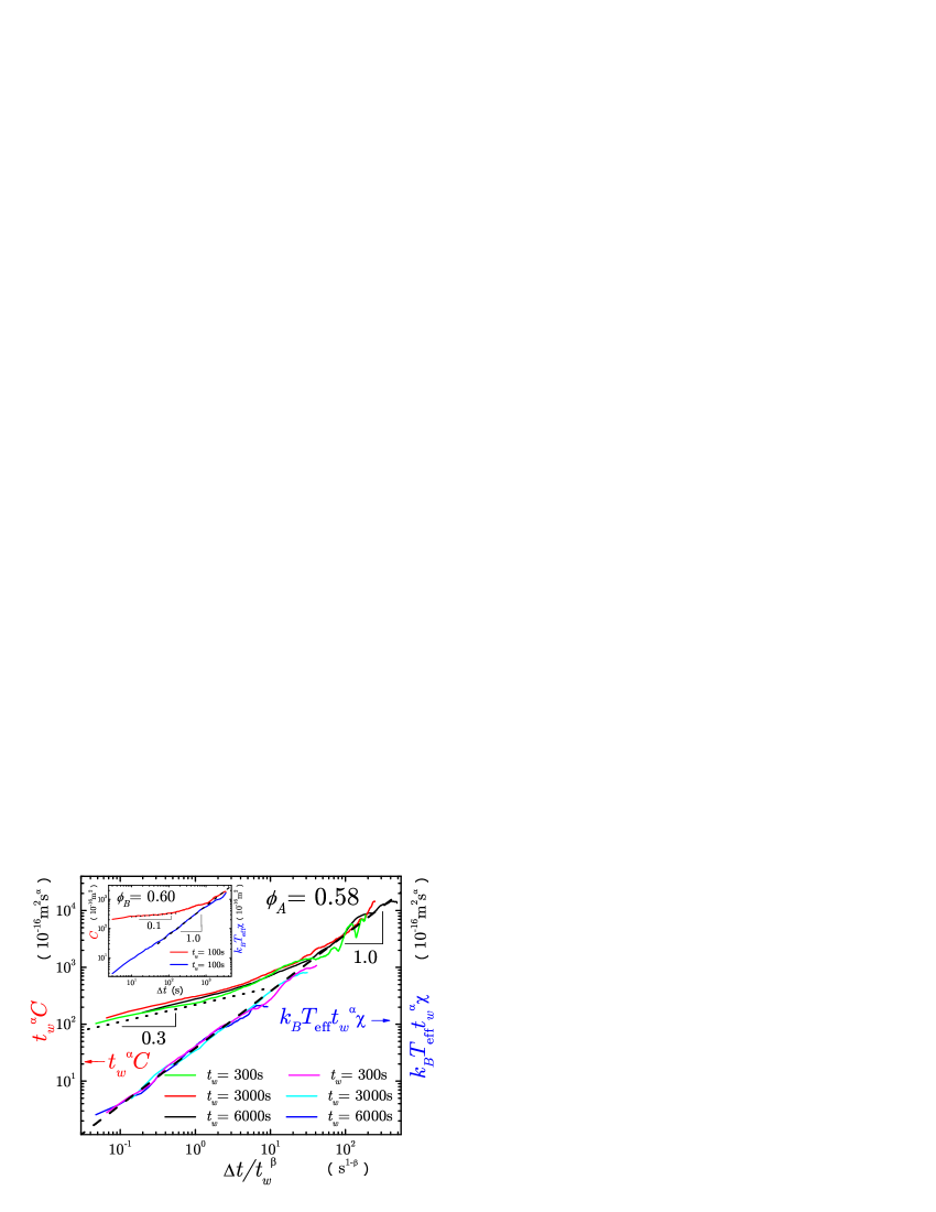
Figure 4: Scaling plot of sample A for the scaled autocorrelation, ${t_{w}}^{\alpha}C$, and scaled integrated response, $k_{B}T_{\rm eff}{t_{w}}^{\alpha}\chi$, as a function of the time ratio, $\Delta{t}/{t_{w}}^{\beta}$, for different waiting times. The black dash line is a linear fit which indicates that $T_{\rm eff}=690K$. The inset is a plot of sample B for autocorrelation, $C$, and integrated response, $k_{B}T_{\rm eff}\chi$, as a function of $\Delta{t}$ at $t_{w}=100s$. The black dash line is a linear fit which indicates that $T_{\rm eff}=1600K$.

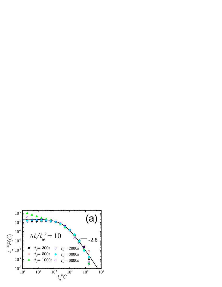
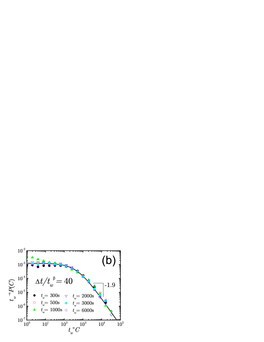
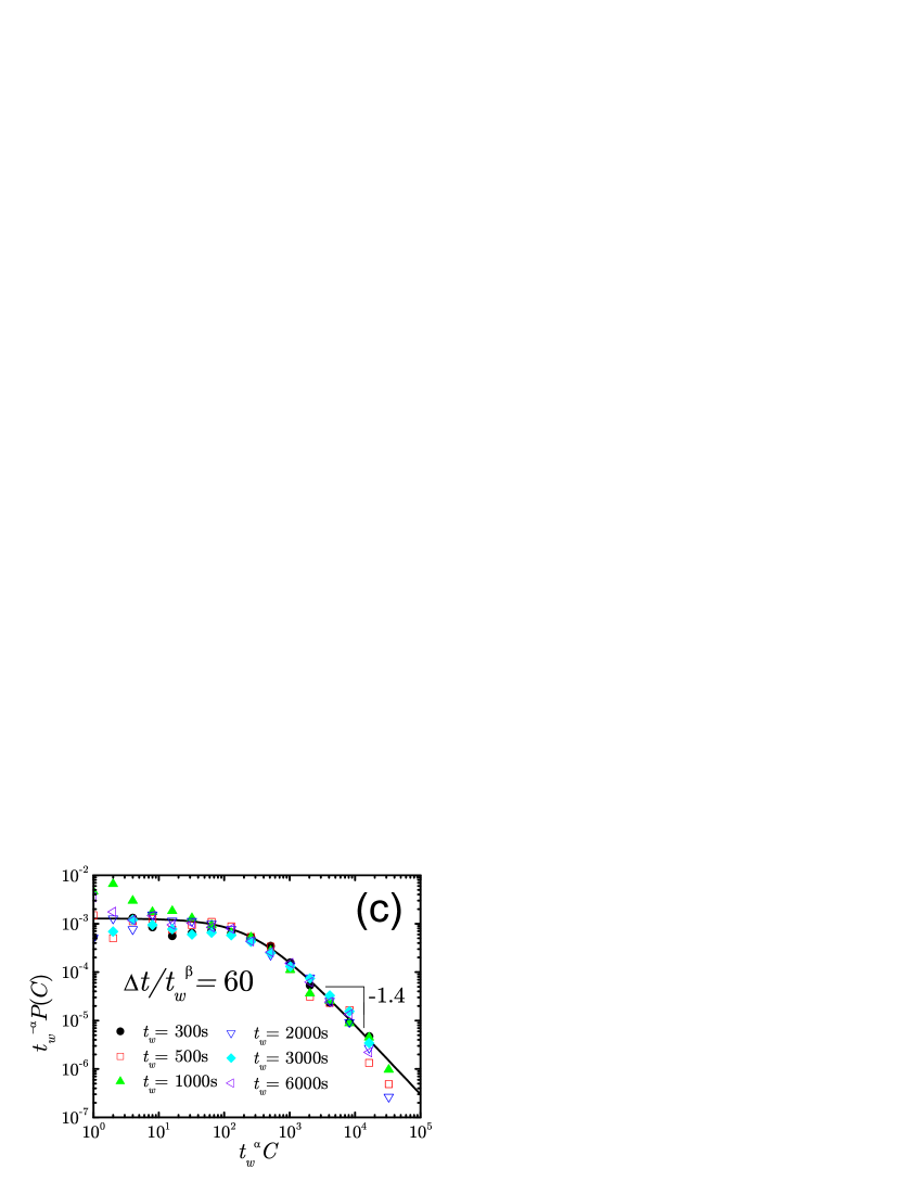
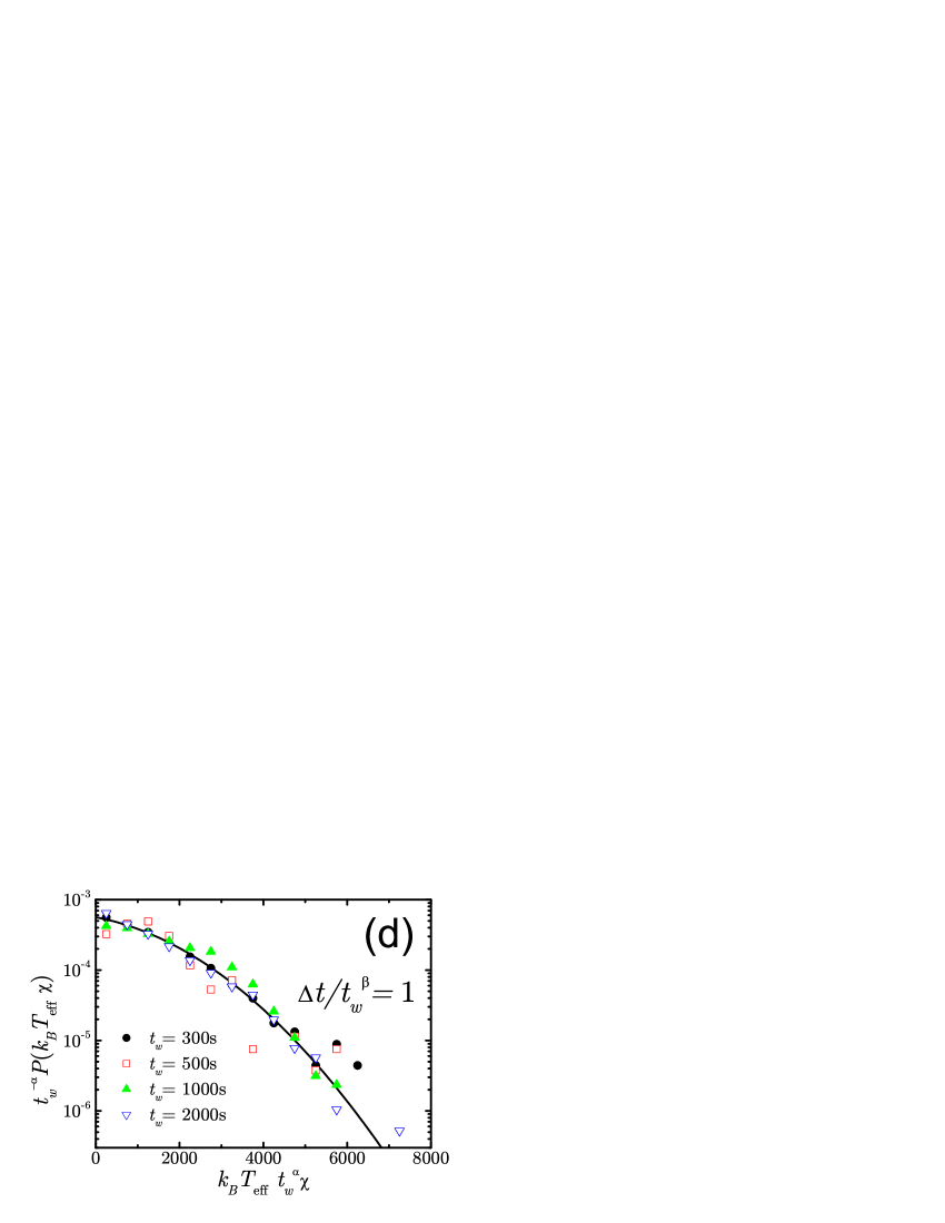
Figure 5: (a) Scaled $\langle x_{12}\rangle$ as a function of scaled $r_{01}$ for given ratio $\Delta t/t_{w}^{\beta}=10$. The linear part for different $t_{w}$ and $\Delta t$ are coincident and well described as $t_{w}^{\alpha/2}\langle x12\rangle=(-0.28)t_{w}^{\alpha/2}r_{01}$ , indicated by the dashed line. (b) Probability distribution function(PDF) of the scaled local correlations for the ratios $\Delta t/t_{w}^{\beta}=1$. (c) Probability distribution function(PDF) of the scaled local correlations for the ratios $\Delta t/t_{w}^{\beta}=60$. The inset is a log-log plot of averaged PDF of the scaled local correlations for three ratios $\Delta t/t_{w}^{\beta}=1,10,60$, the tails are coincident and well fitted by power law with a index -1.25. (d) Probability distribution function(PDF) of the scaled local integrated responses for the ratios $\Delta t/t_{w}^{\beta}=1$. The inset is a log-linear plot of averaged PDF of the scaled local integrated responses for the ratios $\Delta t/t_{w}^{\beta}=1$, the tail are well fitted by a Gaussian function $exp(0.955+0.00881x-5.69613x^{2})$.

IV Scaling ansatz for the global correlations and responses.

Insight into the understanding of the slow relaxation can be obtained from the study of the universal dynamic scaling of the observables with $t_{w}$. Based on spin-glass models, different scaling scenarios have been proposed Cugliandolo ; Henkel for correlation and response functions. Our analysis indicates that the observables can be described as

$$\begin{array}[]{ll}C(t_{w}+\Delta t,t_{w})=\langle\Delta x^{2}\rangle/2=t_{w}^{-\alpha}f_{D}(\frac{\Delta t}{{t_{w}}^{\beta}}),\\ \chi(t_{w}+\Delta t,t_{w})=\frac{\langle\Delta x\rangle}{F}=t_{w}^{-\alpha}f_{M}(\frac{\Delta t}{{t_{w}}^{\beta}}),\end{array}$$ (2)

where $f_{D}$ and $f_{M}$ are two universal functions and $\alpha$ and $\beta$ are the aging exponents. Evidence for the validity of these scaling laws is provided in Fig. 4 where the data of the correlation function and the integrated response function collapse onto a master curve when plotted as $t_{w}^{\alpha}C(t_{w}+\Delta t,t_{w})$ and $t_{w}^{\alpha}\chi(t_{w}+\Delta t,t_{w})$ versus $\Delta t/{t_{w}}^{\beta}$. By minimizing the $\sigma^{2}$ value of the difference between the master curve and the data we find that the best data collapse is obtained for the following aging exponents: $\alpha+\beta=0.34\pm 0.05$ and $\beta=0.48\pm 0.05$. We find (Fig. 4) that the scaling functions satisfy the following asymptotic behavior:

$$f_{D}(y)\sim f_{M}(y)\sim y,$$ (3)

in agreement with the fact that the motion of the particles is diffusive at long times, $\langle\Delta x^{2}\rangle\sim\Delta t$, and the existence of a well-defined mobility, respectively. Therefore at long times, both the correlation and response functions display the same power law decay:

$$\begin{array}[]{ll}C(t_{w}+\Delta t,t_{w})\sim t_{w}^{-(\alpha+\beta)}\Delta t,\\ \chi(t_{w}+\Delta t,t_{w})\sim t_{w}^{-(\alpha+\beta)}\Delta t.\end{array}$$ (4)

The result $C(t_{w}+\Delta t,t_{w})\sim\chi(t_{w}+\Delta t,t_{w})\sim t_{w}^{-0.34}$ indicates $D(t_{w})\sim M(t_{w})\sim t_{w}^{-0.32}$. For short times, the MSD scaling function crosses over to a sub-diffusive behavior of the particles. We obtain, $\langle x^{2}(t_{w}+\Delta t,t_{w})\rangle\sim t_{w}^{-\alpha}(\Delta t/t_{w}^{\beta})^{0.3}=t_{w}^{-0.004}\Delta t^{0.3}$. Since the trapping time corresponds to the size of the cages denoted by $q(t_{w})$, we can determine the cage dependence on $t_{w}$ as $q(t_{w})\sim t_{w}^{-0.002}$. The resulting exponent is so small that we can say that the cages are not evolving with the waiting time, within experimental uncertainty. Furthermore, the scaling ansatz of Eq. (2) indicates that the relaxation time of the cages scales as $\tau(t_{w})\sim t_{w}^{\beta}$ since this is the time when the sub-diffusive behavior crosses-over to the long time diffusive regime.

We find that the scaling forms of the correlations and responses are not consistent with p-spin models. Based on invariance properties under time reparametrization, spin-glass models predict a general scaling form $C_{\rm ag}(t,t_{w})=C_{\rm ag}(h(t)/h(t_{w}))$, where $h(t)$ is a generic monotonic function Cugliandolo . We find that the scaling of our observables cannot be collapsed with the ratio $h(t)/h(t_{w})$. The scaling with $h(t)/h(t_{w})$ is expected for system in which the correlation function saturates at long times Cug_Dou . On the other hand, our system is diffusive, and the studied correlation function is not bounded. Indeed, similar scaling as in our system has been found in the aging dynamics of anther unbounded system: an elastic manifold in a disordered media Bustingorry . The suggestion is that this problem and the particle diffusing in a colloidal glass may belong to the same universality class. Furthermore our results can be interpreted in terms of the droplet picture of the aging of spin glass, where the growth of the dynamical heterogeneities control the aging.

V Local fluctuations of autocorrelations and responses.

Previous work has revealed the existence of dynamical heterogeneities, associated with the cooperative motion of the particles, as a precursor to the glass transition as well as in the glassy state Kegel ; Weeks_sci ; Weeks_aging ; Kob . Instead of the average global quantities studied above, the existence of dynamical heterogeneities requires a microscopic insight into the structure of the glassy. Earlier studies focused mainly on probability distributions of the particles displacement near the glass transition. More recent analytical work in spin glasses Castillo shows that the probability distribution function (PDF) of the local correlation $P(C)$ and the local integrated response $P(\chi)$ could reveal essential features of the dynamical heterogeneities.

Here we perform a systematic study of $P(C)$ and $P(\chi)$ in sample A, and the resulting PDFs are shown in Fig. 5. The scaling ansatz of Eq. (2) implies that $P(C)$ and $P(\chi)$ should be collapsed by rescaling the time $\Delta t$ by $t_{w}^{\beta}$ and the local fluctuations by $t_{w}^{\alpha}$. Indeed, this scaling ansatz provides the correct collapse of all the local fluctuations captured by the PDFs, as shown in Fig. 5a, 5b and 5c for $P(C)$ and in Fig. 5d for $P(\chi)$.

The PDF of the autocorrelation function displays a universal behavior following a modified power-law

$$t_{w}^{-\alpha}P(C)\propto(t_{w}^{\alpha}C+C_{0})^{-\lambda},$$ (5)

where $C_{0}$ and $\lambda$ only depend on the time ratio $\Delta t/t_{w}^{\beta}$. For the smaller values of $C$ ($C<t_{w}^{-\alpha}C_{0}$), the existence of a flat plateau in $P(C)$ indicates that the tracers are confined in the cage. For larger values of $C$, the salient feature of the PDF is the very broad character of the distribution, with an asymptotic behavior $P(C)\sim C^{-\lambda}$. This large deviation from a Gaussian behavior is a clear indication of the heterogeneous character of the dynamics. Furthermore, the exponent $\lambda$ decreases from 2.6 to 1.4 with the time ratio $\Delta t/t_{w}^{\beta}$ ranging from 10 to 60. We notice that $\lambda=2$ corresponds to the crossover between the short-time and long-time regime in Fig. 4, where $\Delta t/t_{w}^{\beta}\approx 40$. The significance of $\lambda=2$ is seen in the integral $\int P(C)CdC$. For $\lambda>2$ ($\Delta t/t_{w}^{\beta}<40$) the plateau dominates over the power law tail in the integral and the dynamics is less heterogeneous. For $\lambda<2$ ($\Delta t/t_{w}^{\beta}>40$) the power law tail dominates and this regime corresponds to the highly heterogeneous long-time regime.

On the contrary, $P(\chi)$, shown in Fig. 5d, displays a different behavior. The fluctuations are more narrow and the PDF can be approximated by a Gaussian. This is consistent with the fact that we did not find cage dynamics for the global response. Moreover, numerical simulations of spin-glass models Castillo seem to indicate a narrower distribution as found here.

VI Scaling behavior of local fluctuations

The local correlation function $C$ and local integrated response function $\chi$ studied here are calculated from each individual tracer trajectory. In a condensed colloidal sample, the tracer trajectories are always confined at a local position. Therefore, the correlation $C$ and response $\chi$ for an individual particle can be regarded as the coarse-grained local fluctuations of the observables as investigated in Castillo .

Furthermore, in order to improve the statistics of our results, the PDF $P(C)$ is calculated not only for all the tracers, but also over a time interval much smaller than the age of the system. In practice, we calculate the $i-$th tracer’s local correlation function as $C_{i}(t_{w}+\Delta t,t_{w})$. At a given $\Delta t$, we open a small time window $[\Delta t-t_{s},\Delta t+t_{s}]$ ($t_{s}\ll\Delta t$) and count all the $C_{i}(t_{w}+\Delta t_{j},t_{w})$ with $\Delta t_{j}\in[\Delta t-t_{s},\Delta t+t_{s}]$ into the statistics of $P(C)$. The calculated $P(C)$ is a mixture of the local and the temporal fluctuations of the observables. Similar technique is performed to calculate $P(\chi)$.

Next we derive the scaling law for the PDF of the local correlation function. Let us first recall the scaling behavior of the global correlation function in Eq. (2),

$$t_{w}^{\alpha}\overline{C(t_{w}+\Delta t,t_{w})}=f_{D}({\Delta t}/{{t_{w}}^{\beta}}),$$ (6)

where we add a bar to $\overline{C}$ to distinguish the global correlations from the local $C$. The average is taken over all the tracer particles. We can rewrite the global correlation function as the integration of the PDF $P(C)$ as:

$$\overline{C}=\int P(C)CdC.$$ (7)

Furthermore, we obtain the relation of $f_{D}$ and $P(C)$ by substituting Eq. (7) into Eq. (6):

$$f_{D}({\Delta t}/{{t_{w}}^{\beta}})=t_{w}^{\alpha}\overline{C}=\int t_{w}^{-\alpha}P(C)(t_{w}^{\alpha}C)d(t_{w}^{\alpha}C).$$ (8)

For a given ${\Delta t}/{{t_{w}}^{\beta}}$, $f_{D}$ is equal to a constant, and Eq. (8) requires that $t_{w}^{-\alpha}P(C)$ should only depend on $t_{w}^{\alpha}C$. In other words, $t_{w}^{-\alpha}P(C)$ is a function of ${\Delta t}/{{t_{w}}^{\beta}}$ and $t_{w}^{\alpha}C$. Then we define $F_{D}$ as:

$$F_{D}(t_{w}^{\alpha}C,\Delta t/t_{w}^{\beta})=t_{w}^{-\alpha}P(C).$$ (9)

A similar formula can be obtained for $P(\chi)$. Eventually, we obtain the scaling ansatz of $P(C)$ and $P(\chi)$ shown in Fig. 5:

$$\begin{array}[]{ll}P(C)&=t_{w}^{\alpha}F_{D}(t_{w}^{\alpha}C,\Delta t/t_{w}^{\beta}),\\ P(\chi)&=t_{w}^{\alpha}F_{M}(t_{w}^{\alpha}\chi,\Delta t/t_{w}^{\beta}),\end{array}$$ (10)

where the universal functions $F_{D}(x,y)$ and $F_{M}(x,y)$ satisfy

$$\begin{array}[]{ll}\int F_{D}(x,y)dx=f_{D}(y),\\ \int F_{M}(x,y)dx=f_{M}(y).\end{array}$$ (11)

VII Study of the PDF of the autocorrelation function

The PDF of the autocorrelation function follows a modified power law $t_{w}^{-\alpha}P(C)\propto(t_{w}^{\alpha}C+C_{0})^{-\lambda}$, as we see in Figs. 5a, 5b and 5c. From Eq. (8), we have

$$\begin{split}t_{w}^{\alpha}\overline{C}&=\int_{0}^{C_{cut}}t_{w}^{-\alpha}P(C)(t_{w}^{\alpha}C)d(t_{w}^{\alpha}C)\\ &=\frac{\int_{0}^{C_{cut}}(x+C_{0})^{-\lambda}xdx}{\int_{0}^{C_{cut}}(x+C_{0})^{-\lambda}dx}.\end{split}$$ (12)

The cutoff $C_{cut}$ ($C_{cut}\gg C_{0}$) is introduced to make the integral converge and we always take $\lambda\geq 1$, then

$$t_{w}^{\alpha}\overline{C}=\frac{C_{0}}{\lambda-2}[1-(\lambda-1)(\frac{C_{cut}}{C_{0}}+1)^{2-\lambda}].$$ (13)

For $\lambda>2$, the last term in Eq. (13) is negligible and $t_{w}^{\alpha}\overline{C}\approx C_{0}/(\lambda-2)$ mainly depends on the short-time parameter $C_{0}$. For $\lambda<2$, we have $t_{w}^{\alpha}\overline{C}\approx\frac{\lambda-1}{2-\lambda}C_{0}(\frac{C_{cut}}{C_{0}})^{2-\lambda}$ and the long-time parameter $C_{cut}$ dominates.

Following the previous discussion of $P(C)$, we define the $i$-th tracer’s local correlation function as:

$$C_{i}(t_{w}+\Delta t,t_{w})=\langle\Delta x(t_{w}+\Delta t,t_{w})^{2}\rangle_{i}/2,$$ (14)

where the average $\langle...\rangle_{i}$ is calculated for only the $i$-th tracer’s trajectory by opening a small time window $[\Delta t-t_{s},\Delta t+t_{s}]$ ($t_{s}\ll\Delta t$) at a given $\Delta t$, and counting all the $C_{i}(t_{w}+\Delta t_{j},t_{w})$ with $\Delta t_{j}\in[\Delta t-t_{s},\Delta t+t_{s}]$ into the statistics of $P(C)$. We should note that if there is no average $\langle...\rangle_{i}$, $P(C)$ can be reduced to a simple form:

$$P(C)=P(\langle\Delta x^{2}\rangle_{i}/2)\xrightarrow{\langle...\rangle_{i}\rightarrow 0}P(\Delta x^{2}/2).$$ (15)

This form can be further reduced since

$$P(\Delta x^{2}/2)d(\Delta x^{2}/2)=P(\Delta x)dx,$$ (16)

therefore at the limit of the average $\langle...\rangle_{i}\rightarrow 0$,

$$P(C)=P(\langle\Delta x^{2}\rangle_{i}/2)\xrightarrow{\langle...\rangle_{i}\rightarrow 0}P(\Delta x^{2}/2)=P(\Delta x)/{\Delta x}.$$ (17)

Therefore our $P(C)$ is related to the probability $P(\Delta x)$ usually studied in previous works Weeks_sci . The reader with enough endurance to have reached this point in the paper may realize the apparent contradiction between our power-law scaling and the typical stretched exponential behaviour found in other studies of local fluctuations. In this regard we may first say that previous work considered the supercooled regime while we work in the glassy regime. Thus, both regimes may show different type of scaling. When we analyze the scaling of $P(\Delta x)$ in our glassy system we find that it can be approximately fitted by both a broad tail power law behavior for large $\Delta x$, consistent with equation 5, but also by a stretched exponential, which is consistent with previous works Weeks_sci for the supercooled regime. On the hand $P(\langle\Delta x^{2}\rangle_{i}/2)$ can not be fitted by stretch exponential and it is only fitted by the power-law scaling. Therefore, we conclude that the power scaling should be the proper scaling for $P(\Delta x)$ and $P(C)$ in the glassy regime.

VIII Summary

We have presented experimental results on the scaling behavior of the fluctuations in an aging colloidal glass. The power-law scaling found to describe the transport indicates the slow relaxation of the system. A universal scaling form is found to describe all the observables. That is, not only the global averages, but also the local fluctuations. The scaling ansatz, however, cannot be described under present models of spin-glasses, but it is more akin to that observed in elastic manifolds in random environments suggesting that our system may share the same universality class.

References

- (1) Pusey, P. N. & van Megen, W. Phase behavior of concentrated suspensions of nearly hard colloidal spheres. Nature 320, 340-342 (1986).
- (2) Cugliandolo, L. F. in Slow Relaxations and Nonequilibrium Dynamics in Condensed Matter, Barrat, J. -L. et al. (eds.) (Springer-Verlag, 2002).
- (3) Struik, L. C. E. in Physical Ageing in Amorphous Polymer and other Materials, (Elsevier, Houston, 1978).
- (4) Cugliandolo, L. F. & Kurchan, J. Analytical solution of the off-equilibrium dynamics of a long-range spin-glass model Phys. Rev. Lett. 71, 173-176 (1993).
- (5) Bouchaud, J. -P., Cugliandolo, L. F., Kurchan, J., & Mézard, M. in Spin-Glasses and Random Fields, (World Scientific, 1998).
- (6) Kegel, W. K. & van Blaaderen, A. Direct observation of dynamical heterogeneities in colloidal hard-sphere suspensions. Science 287, 290-293 (2000).
- (7) Weeks, E. R., Crocker, J. C., Levitt, A. C., Schofield, A. & Weitz, D. A. Three-dimensional direct imaging of structural relaxation near the colloidal glass transition. Science 287, 627-631 (2000).
- (8) Song, C., Wang, P. & Makse, H. A. Experimental measurement of an effective temperature for jammed granular materials. Proc. Nat. Acad. Sci. 102, 2299-2304 (2005).
- (9) Amblard, F., Yurke, B., Pargellis, A. N. & Leibler, S. A magnetic manipulator for studying local rheology and micromechanical properties of biological systems. Rev. Sci. Instrum. 67, 818-827 (1996).
- (10) Habdas, P. et al. Forced motion of a probe particle near the colloidal glass transition. Europhys. Lett. 67, 477-483 (2004).
- (11) Henkel, M., Pleimling, M., Godrèche, G. & Luck, J. -M. Aging, phase ordering, and conformal invariance. Phys. Rev. Lett. 87, 265701 (2001).
- (12) Cugliandolo, L. F., Kurchan, J., & Doussal, P. L. Large Time Out-of-Equilibrium Dynamics of a Manifold in a Random Potential. Phys. Rev. Lett. 76, 2390-2393 (1996).
- (13) Bustingorry, S., Cugliandolo, L. F., & Dominguez, D. Out-of-Equilibrium Dynamics of the Vortex Glass in Superconductors. Phys. Rev. Lett. 96, 027001 (2006).
- (14) Courtland, R. E., Weeks, E. R. Direct visualization of ageing in colloidal glasses. J. Phys.: Condens. Matter 15, S359-S365 (2003).
- (15) Kob, W., Donati, C., Plimpton, S. J., Poole, P. H., & Glotzer, S. C. Dynamical heterogeneities in a supercooled Lennard-Jones liquid. Phys. Rev. Lett. 79, 2827-2830 (1997).
- (16) Castillo, H. E., Chamon, C., Cugliandolo, L. F. & Kennett, M. P. Heterogeneous aging in spin glasses. Phys. Rev. Lett. 88, 237201 (2002).