A mean field approach for string condensed states

Abstract

We describe a mean field technique for quantum string (or dimer) models. Unlike traditional mean field approaches, the method is general enough to include string condensed phases in addition to the usual symmetry breaking phases. Thus, it can be used to study phases and phases transitions beyond Landau’s symmetry breaking paradigm. We demonstrate the technique with a simple example: the spin-$1$ XXZ model on the Kagome lattice. The mean field calculation predicts a number of phases and phase transitions, including a $z=2$ deconfined quantum critical point.

I Introduction

Recently, several frustrated spin systems have been discovered with the unusual property that their collective excitations are described by Maxwell’s equations. Wen (2002); Motrunich and Senthil (2002); Wen (2003); Moessner and Sondhi (2003); Wen (2004); Hermele et al. (2004) These light-like collective modes can be traced to the highly entangled nature of the ground state. In these systems, the low energy degrees of freedom are not individual spins, but rather string-like loops of spins. The ground state is a coherent superposition of many such string-like configurations - a “string condensate.” It is this “string condensation” in the ground state that is responsible for the emergent photon - just as particle condensation is responsible for the phonon modes in a superfluid. Wen (2003); Levin and Wen (2005a, b, 2006)

While this qualitative picture is relatively clear, quantitative results on string condensation and artificial light are lacking. The above models have only been analyzed in limiting and unrealistic cases. We do not know any realistic systems with emergent photons. The problem is that we are missing a good mean field approach for exotic states. Current mean field theory approaches can only be applied to symmetry breaking states with local order parameters. They are useless for understanding string condensed states which are highly entangled and have nothing to do with symmetry breaking.

In this paper, we address this problem. We describe a mean field approach that can be applied to both symmetry breaking and string condensed states. We hope that this technique can be used to identify conditions under which string condensation may occur, and to help further the experimental search for emergent photons and new states of matter.

In practice, our approach can be thought of as a mean field technique for quantum string (or dimer) models. This technique can be used to estimate the phase diagram of string (or dimer) models, to find the low energy dynamics of the different phases, and to analyze the phase transitions. It can be applied to any quantum spin system with the property that its low energy degrees of freedom are strings or dimers. This includes all the frustrated spin systems cited above.

We demonstrate the technique with a simple example: a spin-$1$ XXZ model on the Kagome lattice Wen (2003):

$$H =J_{1}\sum_{\boldsymbol{I}}(S^{z}_{\boldsymbol{I}})^{2}+J_{2}\sum_{\langle\boldsymbol{I}\boldsymbol{J}\rangle}S^{z}_{\boldsymbol{I}}S^{z}_{\boldsymbol{J}}$$

$$-J_{xy}\sum_{\langle\boldsymbol{I}\boldsymbol{J}\rangle}(S^{x}_{\boldsymbol{I}}S^{x}_{\boldsymbol{J}}+S^{y}_{\boldsymbol{I}}S^{y}_{\boldsymbol{J}})$$ (1)

Here $\boldsymbol{I}$ and $\boldsymbol{J}$ label the sites of the Kagome lattice, and $\sum_{\langle\boldsymbol{I}\boldsymbol{J}\rangle}$ sums over all nearest neighbor sites. This model provides a good testing ground for the method since the low energy dynamics of $H$ is described by a string model in the regime $J_{2}\gg J_{xy}\gg|J_{1}-J_{2}|$.

The mean field calculation predicts a number of interesting phases including string condensed phases with emergent photons. The string condensed phases are ultimately destroyed once instanton fluctuations are included, but several phases and phase transitions remain - including a deconfined quantum critical point.

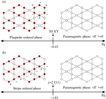
Figure 1: The mean field phase diagram for (a) the XXZ model (I) and (b) the XXZ model with additional next nearest neighbor interactions. The filled circles denote spins with $\langle S^{z}\rangle\neq 0$. The sign of $\langle S^{z}\rangle$ alternates around each plaquette in the plaquette ordered phase and along each stripe in the stripe ordered phase.

The mean field phase diagram for (I) is shown in Fig. 1a. Here, $J=\frac{9J_{xy}^{2}}{J_{2}}+\frac{24J_{xy}^{3}}{J_{2}^{2}}+3(J_{1}-J_{2})$, and $g=\frac{3J_{xy}^{3}}{J_{2}^{2}}$. For large positive $J/g$, the system is in a paramagnetic phase with no broken symmetries, while for large negative $J/g$, the system is in a plaquette ordered phase with broken lattice and spin symmetries. The critical point is in the universality class of the 3D $XY$ model. This is similar to, but slightly different from the phase diagram obtained in LABEL:XM0555. In that paper, the authors also predict a plaquette phase at large negative $J/g$, but their candidate phase is a resonating plaquette phase which has different symmetries from the frozen plaquette phase shown above.

We also study the model (I) with an additional second nearest neighbor interaction $J_{3}\sum_{\langle\langle\boldsymbol{i}\boldsymbol{j}\rangle\rangle}S^{z}_{\boldsymbol{i}}S^{z}_{\boldsymbol{j}}$, $J_{3}/g=0.17$. We find a different phase diagram (Fig. 1b). For large positive $J/g$, the system is in a paramagnetic phase, while for large negative $J/g$ the system is in a stripe ordered phase with broken rotational and spin symmetry. The mean field calculation predicts that the phase transition is a deconfined quantum critical point described by a $U(1)$ gauge theory with dynamical exponent $z=2$. However, we cannot rule out the possibility of a first order phase transition - for either of the two models.

The paper is organized as follows. In section II we describe the string picture for the Kagome model (I). In section III we present the mean field approach and derive the mean field phase diagram for (I). In section IV, we derive the low energy dynamics in each of the phases, and in section V we analyze the phase transitions in the model. The details of the mean field calculation are presented in the Appendix.

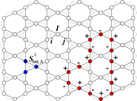
Figure 2: When $J_{1}-J_{2}=J_{xy}=0$, the Kagome XXZ model (I) has an extensive ground state degeneracy. All states satisfying $S^{z}_{\text{tot},\Delta}=\sum_{\boldsymbol{I}\in\Delta}S^{z}_{\boldsymbol{I}}=0$ are ground states. If we view the sites of the Kagome lattice as links of a honeycomb lattice, then the ground states are collections of closed loops of alternating $S^{z}=\pm 1$ on the honeycomb lattice.

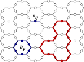
Figure 3: The low energy effective string Hamiltonian (3) is made up of two terms: an operator $n_{\boldsymbol{i}\boldsymbol{j}}$ which is the string occupation number on the link $\boldsymbol{i}\boldsymbol{j}$ and an operator $B_{\boldsymbol{p}}$ which creates (or moves) strings along the boundary of the plaquette $\boldsymbol{p}$.

II String picture

II.1 Effective string model

We will study the XXZ model (I) in the regime $J_{2}\gg J_{xy}\gg|J_{1}-J_{2}|$. In that case the low energy dynamics of $H$ is described by a string model - a close cousin of a quantum dimer model. Wen (2003) To see this, note that the Hamiltonian can be rewritten as

$$H =\frac{J_{2}}{2}\sum_{\Delta}(S^{z}_{\text{tot},\Delta})^{2}+(J_{1}-J_{2})\sum_{\boldsymbol{I}}(S^{z}_{\boldsymbol{I}})^{2}$$

$$-J_{xy}\sum_{\langle\boldsymbol{I}\boldsymbol{J}\rangle}(S^{x}_{\boldsymbol{I}}S^{x}_{\boldsymbol{J}}+S^{y}_{\boldsymbol{I}}S^{y}_{\boldsymbol{J}})$$ (2)

where $S^{z}_{\text{tot},\Delta}=\sum_{\boldsymbol{I}\in\Delta}S^{z}_{\boldsymbol{I}}$, and $\Delta$ runs over the triangles in the Kagome lattice (see Fig. 2).

Suppose that $J_{xy}=J_{1}-J_{2}=0$. In that case, $H$ has an extensive ground state degeneracy: every state satisfying $S^{z}_{\text{tot},\Delta}=0$ for all triangles $\Delta$, is a ground state. To describe these ground states, it is useful to view the sites $\boldsymbol{I}$ of the Kagome lattice as the links of a honeycomb lattice - whose vertices we will label by $\boldsymbol{i}$. One ground state is the state with $S^{z}_{\boldsymbol{I}}=0$ for all links $\boldsymbol{I}$ of the honeycomb lattice. Another ground state can be obtained by alternately increasing and decreasing $S^{z}_{\boldsymbol{I}}$ along a closed loop on the honeycomb lattice. In general all the ground states are of this form: they consist of collections of closed loops of alternating $S^{z}_{\boldsymbol{I}}=\pm 1$ superimposed on a background of $S^{z}_{\boldsymbol{I}}=0$. (see Fig. 2).

These states can be thought of as configurations of oriented strings on the honeycomb lattice. To do this precisely, we pick an $A$ and $B$ sublattice of the honeycomb lattice. For any link $\boldsymbol{I}=\langle\boldsymbol{i}\boldsymbol{j}\rangle$, we say that $\boldsymbol{I}$ contains an oriented string pointing from $\boldsymbol{i}\in A$ to $\boldsymbol{j}\in B$ if $S^{z}_{\boldsymbol{I}}=+1$, and from $\boldsymbol{j}$ to $\boldsymbol{i}$ if $S^{z}_{\boldsymbol{I}}=-1$. We say the link is empty if $S^{z}_{\boldsymbol{I}}=0$ (see Fig. 3). Then the ground states described above are in exact correspondence with configurations of oriented closed strings on the honeycomb lattice.

Now consider the case where $J_{xy},J_{1}-J_{2}$ are small but nonzero. These terms will split the extensive degeneracy described above. The splitting can be described in degenerate perturbation theory by a low energy effective string Hamiltonian $H_{eff}$. Working to third order in $J_{xy}/J_{2}$ and assuming $J_{xy}\gg|J_{1}-J_{2}|$ we find:

$$H_{eff}=\frac{J}{3}\sum_{\boldsymbol{i}\boldsymbol{j}}n_{\boldsymbol{i}\boldsymbol{j}}-\frac{g}{2}\sum_{\boldsymbol{p}}(B_{\boldsymbol{p}}+h.c)\\$$ (3)

where $J=\frac{9J_{xy}^{2}}{J_{2}}+\frac{24J_{xy}^{3}}{J_{2}^{2}}+3(J_{1}-J_{2})$, and $g=\frac{3J_{xy}^{3}}{J_{2}^{2}}$. Here, the two operators, $n_{\boldsymbol{i}\boldsymbol{j}},B_{\boldsymbol{p}}$ are operators that act on oriented string states. The operator $n_{\boldsymbol{i}\boldsymbol{j}}$ is the string occupation number on the link $\boldsymbol{i}\boldsymbol{j}$. That is, for any string state $|X\rangle$, $n_{\boldsymbol{i}\boldsymbol{j}}|X\rangle=|X\rangle$ if there is a string on $\langle\boldsymbol{i}\boldsymbol{j}\rangle$ with orientation $\boldsymbol{i}\rightarrow\boldsymbol{j}$ and $n_{\boldsymbol{i}\boldsymbol{j}}|X\rangle=0$ otherwise. The operator $B_{\boldsymbol{p}}$ acts on the six links along the boundary of the plaquette $\boldsymbol{p}$. It’s action is given by

$$B_{\boldsymbol{p}}\left|\begin{matrix}\includegraphics[height=43.36243pt]{Bp1.eps}\end{matrix}\right\rangle=\left|\begin{matrix}\includegraphics[height=43.36243pt]{Bp2.eps}\end{matrix}\right\rangle$$

where $a=0$ denotes the empty link and $a=+1$ $(-1)$ denotes the link with a string oriented clockwise (counterclockwise) with respect to $\boldsymbol{p}$ (see Fig. 3). If any of $a,...,f=+1$, $B_{\boldsymbol{p}}$ annihilates the state: $B_{\boldsymbol{p}}|a,b,c,d,e,f\rangle=0$. One can think of $B_{\boldsymbol{p}}$ as being analogous to the dimer flip operators in quantum dimer models.

In the remainder of the paper, we will focus entirely on this low energy effective string model (3). While our discussion will focus on strings we would like to emphasize that the results tell us about the physics of the simple spin model (I).

II.2 Possible phases

The two terms in the Hamiltonian (3) have a simple physical interpretation in the string language. The first term, $J/3\sum_{\boldsymbol{i}\boldsymbol{j}}n_{\boldsymbol{i}\boldsymbol{j}}$ is a string tension which penalizes strings for being long. The second term, $g/2\sum_{\boldsymbol{p}}(B_{\boldsymbol{p}}+h.c)$ is a string kinetic energy term. It makes the strings fluctuate and gives them dynamics.

We are interested in the phase diagram of this model. We will focus on the case $g>0$ for simplicity. There are three basic regimes to consider: $J/g\gg 1$, $|J|/g\ll 1$ and $-J/g\gg 1$.

When $J/g\gg 1$ the string tension term dominates. In this regime, the physics of (3) is clear. We expect the ground state to be the vacuum state with a few small strings; the system is in a “small string” phase. On the other hand, when $|J|/g\ll 1$, the string kinetic energy dominates. In this regime, the behavior of (3) is less straightforward. One plausible scenario is that kinetic energy term favors a ground state which is a superposition of many large strings - a “string condensed” state. (see Fig. 4) However, it is also possible that the energetics favor a string crystal phase, or even a small string phase. In the final regime, when $-J/g\gg 1$, the negative string tension favors “fully packed” string states - states where every point on the honeycomb lattice is contained in a string. Again, the physics is not clear. It is possible that the system enters a fully packed string crystal phase - but it could equally well realize a fully packed string liquid state.

Clearly, even the qualitative phase diagram for the string model (3) is not obvious. There are many potentially competing phases with very different properties. We would like to have a method for determining which of these phases are actually realized and for what parameters. It would be particularly useful to know in what region the string condensed phase occurs, if at all - since this phase may contain gapless photon-like modes. The mean field technique described below accomplishes this task.

Figure 4: One possible phase diagram for the string model (3). The string orientations have been omitted for clarity.

III Mean field approach

In this section, we describe a mean field technique for quantitatively computing the phase diagram for the string model (3). As we will see later, it can also be used to derive a low energy effective Lagrangian for each of the phases, and to analyze the phase transitions. We would like to mention that similar approaches have been used to study lattice gauge theory. Boyanovsky et al. (1980); Horn and Weinstein (1982)

III.1 Variational states

Our approach is variational - we define a large class of variational string wave functions, and then minimize their energy $\langle H\rangle$. Let us begin by describing the variational wave functions. The wave functions $\Psi$ have a large number of variational parameters $\{z_{\boldsymbol{i}\boldsymbol{j}}\}$ indexed by the oriented links $\boldsymbol{i}\boldsymbol{j}$ of the honeycomb lattice. For each set of $\{z_{\boldsymbol{i}\boldsymbol{j}}\}$, the corresponding wave function $\Psi_{\{z\}}$ is defined by

$$\Psi_{\{z\}}(X)=\prod_{\boldsymbol{i}\boldsymbol{j}}z_{\boldsymbol{i}\boldsymbol{j}}^{n_{\boldsymbol{i}\boldsymbol{j}}}$$ (4)

where $n_{\boldsymbol{i}\boldsymbol{j}}$ is the occupation number of the oriented link $\boldsymbol{i}\boldsymbol{j}$ in the oriented string configuration $X$. We can see that $z_{\boldsymbol{i}\boldsymbol{j}},z_{\boldsymbol{j}\boldsymbol{i}}$ are string fugacities on the link $\langle\boldsymbol{i}\boldsymbol{j}\rangle$ for the two different string orientations.

The above variational wave function (4) can accommodate many different kinds of states - including both string crystals and string liquids. If $z_{\boldsymbol{i}\boldsymbol{j}}$ is periodic, $\Psi_{\{z\}}$ is a symmetry breaking string crystal state; if $z_{\boldsymbol{i}\boldsymbol{j}}$ is constant for all $\boldsymbol{i}\boldsymbol{j}$, then $\Psi_{\{z\}}$ is a string liquid state. The variational states $\Psi_{\{z\}}$ can even access the two types of string liquids described in the previous section - small string states and string condensed states - and can capture the distinction between them.

To see this, consider a string liquid state with $z_{\boldsymbol{i}\boldsymbol{j}}=\alpha$. The properties of the state $\Psi_{\alpha}$ can be deduced from the properties of the classical loop gas with statistical weight $P(X)=|\Psi_{\alpha}(X)|^{2}=\alpha^{2L(X)}$ (here $L(X)$ is the total length of all the loops in $X$). This loop gas is the classical $O(2)$ loop gas on the honeycomb lattice and has been solved exactly. It is known that the loop gas has two phases separated by a phase transition at $\alpha_{c}=2^{-1/4}\approx 0.84$. Domany et al. (1981) When $\alpha<\alpha_{c}$, the classical loop gas is in a “small loop” phase, where the typical loop size is some finite length scale $\xi$. On the other hand, when $\alpha>\alpha_{c}$, the loop gas enters a phase with large loops of arbitrarily large size. Intuitively, this means that the states $\Psi_{\alpha}$ with $\alpha<\alpha_{c}$ should be regarded as small string states, while the states with $\alpha>\alpha_{c}$ should be regarded as string condensed states.

In the same way it is not hard to see that the wave functions $\Psi_{\{z\}}$ can even accommodate simultaneous symmetry breaking order and string condensation. Consider, for example, the case where $z_{\boldsymbol{i}\boldsymbol{j}}$ is large and nearly constant, but has a small periodic position dependence. In that case, $\Psi_{\{z\}}$ will exhibit both translational symmetry breaking and string condensation.

III.2 Defining string condensed states

In the preceding section, we relied on an intuitive picture of string condensed states. Here we make our language more precise - formally defining which variational states $\Psi_{\{z\}}$ we regard as string condensed.

To state our definition, we place the wave function $\Psi_{\{z\}}$ on a thermodynamically large cylinder and consider the classical loop gas associated with $|\Psi_{\{z\}}|^{2}$. We define a quantity $\rho_{s}$ by

$$\rho_{s}=\langle W^{2}\rangle-\langle W\rangle^{2}$$ (5)

where the expectation values are taken with respect to the classical loop gas, and $W$ is the winding number, e.g. $W$ counts the number of times the loops wind around the cylinder. Our definition is that the state $\Psi_{\{z\}}$ is string condensed if $\rho_{s}>0$ and not string condensed if $\rho_{s}=0$ in the thermodynamic limit. Thus, $\rho_{s}$ can be thought of as a (non-local) order parameter for string condensation.

The motivation for this definition is twofold. First, it captures our intuitive picture of string condensation: states with large fluctuating loops (such as $\Psi_{\alpha}$, $\alpha>\alpha_{c}$) have $\rho_{s}>0$ while other states (such as $\Psi_{\alpha}$, $\alpha<\alpha_{c}$) have $\rho_{s}=0$. Second, it agrees with the expected low energy physics of string condensed states. We will see that states with $\rho_{s}>0$ generically have a gapless linearly dispersing photon-like mode (neglecting instanton effects), while other states are gapped.

In addition to clarifying our discussion of string condensation, $\rho_{s}$ can be used in numerical simulations to distinguish string condensed $\Psi_{\{z\}}$ from normal $\Psi_{\{z\}}$. As a demonstration, we have computed $\rho_{s}$ numerically for the liquid states, $z_{\boldsymbol{i}\boldsymbol{j}}=\alpha$ and found that the transition from small string states to string condensed states occurs at $\alpha_{c}\approx 0.82$ (Fig. 5). In this particular case this computation was unnecessary, since the transition point was already known analytically: $\alpha_{c}=2^{-1/4}\approx 0.84$. However, in more complicated cases (such as states with non-uniform $z_{\boldsymbol{i}\boldsymbol{j}}$), such a numerical calculation would be necessary.

Finally, we would like to mention a physical interpretation of $\rho_{s}$ which will prove useful later. This interpretation is based on the duality between the classical $O(2)$ loop gas and the classical (2D) $XY$ model. Domany et al. (1981) This duality maps the small loop phase of the classical loop gas onto the disordered phase of the $XY$ model, the large loop phase onto the (algebraically) ordered phase of the $XY$ model, and the transition at $\alpha=\alpha_{c}$ onto the Kosterlitz-Thouless transition. Under this duality, the quantity $\rho_{s}$ corresponds to the superfluid stiffness in the dual $XY$ model. This means that our previous definition of string condensed states can be rephrased as: $\Psi_{\{z\}}$ is string condensed if and only if the $XY$ model dual to the loop gas $|\Psi_{\{z\}}^{2}|$ is in the ordered phase.

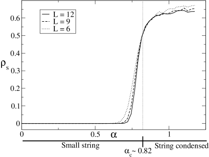
Figure 5: Monte Carlo results for $\rho_{s}$ as a function of $\alpha$, obtained on $6\times 6$, $9\times 9$ and $12\times 12$ lattices. In the thermodynamic limit, $\rho_{s}$ vanishes for the small string states and then jumps to a finite non-zero value for the string condensed states. We estimate the critical point $\alpha_{c}\sim 0.82$ as the value of $\alpha$ where the three finite size curves intersect.

III.3 Mean field phase diagram

The mean field phase diagram can be obtained by minimizing the ground state energy $\langle H\rangle$ over all states $\Psi_{\{z\}}$, and then identifying the quantum phase associated with the minimum energy $\Psi_{\{z\}}$. Energy expectation values can be obtained in a number of ways - we compute them numerically using a variational Monte Carlo method.

We have applied this technique to (3), using the energy minimization procedure described in Appendix A. We find the mean field phase diagram shown in Fig. 6a. We find that when $J/g>0.27$, the system is in a small string liquid phase. When $-0.43<J/g<0.27$ the system is in a string condensed liquid phase. When $J/g<-0.43$, the system enters a phase with simultaneous string condensation and plaquette order. We have not executed systematic numerics beyond this point but we believe that when $J/g$ becomes sufficiently large and negative, the string condensation is destroyed, and the system enters a phase with plaquette order and no string condensation. (See Appendix B for details on how these results were obtained).

As we will show later, the true phase diagram is different from the mean field phase diagram due to instanton effects. Once these are taken into account, the two string condensed phases are destroyed, and only the small string and plaquette ordered phases remain (Fig. 6b). This is similar to, but slightly different from the phase diagram obtained in LABEL:XM0555. In that paper, the authors predict a resonating plaquette phase (Fig. 8b) at large negative $J/g$, while our mean field phase diagram predicts a frozen plaquette phase (Fig. 8a). The two phases have the same translational symmetry group, but different symmetries under spatial and spin rotations.

We have also computed the mean field phase diagram from the model (I) with an additional next nearest neighbor interaction $J_{3}\sum_{\langle\langle\boldsymbol{i}\boldsymbol{j}\rangle\rangle}S^{z}_{\boldsymbol{i}}S^{z}_{\boldsymbol{j}}$, $J_{3}/g=0.17$. We find that the phase diagram shown in Fig. 7a. When $J/g>-0.11$, the system is in a small string liquid phase, while when $-1.83<J/g<-0.11$ the system is in a string condensed liquid phase. When $J/g<-1.83$, the system enters a phase with simultaneous string condensation and stripe order (Fig. 9). Instanton effects ultimately destroy the two string condensed phases leaving only the small string phase and the stripe ordered phase (Fig. 7b). However, as we will see in section (V), an interesting deconfined quantum critical point remains - the transition between the small string and stripe ordered phases.

Figure 6: (a) The phase diagram obtained from the mean field approach. (b) The phase diagram after instanton effects have been included. The string condensed phases are destroyed and only two phases remain.

Figure 7: (a). The mean field phase diagram for the XXZ model with a small second nearest neighbor interaction $J_{3}\sum_{\langle\langle\boldsymbol{i}\boldsymbol{j}\rangle\rangle}S^{z}_{\boldsymbol{i}}S^{z}_{\boldsymbol{j}}$, $J_{3}/g=0.17$. (b). The phase diagram after instanton effects have been included.

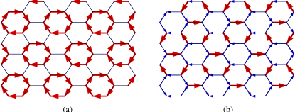
Figure 8: The mean field calculation predicts (a) frozen plaquette order for $J/g<-0.43$. Previous work Xu and Moore (2005) has suggested (b) resonating plaquette order. The two orders are shown above: the thickness of the bonds indicates the size of $z_{\boldsymbol{i}\boldsymbol{j}}\cdot z_{\boldsymbol{j}\boldsymbol{i}}$ while the arrows indicate the relative size of $z_{\boldsymbol{i}\boldsymbol{j}}$ and $z_{\boldsymbol{j}\boldsymbol{i}}$.

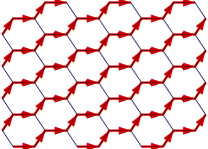
Figure 9: The addition of a second nearest neighbor interaction leads to a stripe ordered phase, depicted above. The thickness of the bonds indicates the size of $z_{\boldsymbol{i}\boldsymbol{j}}\cdot z_{\boldsymbol{j}\boldsymbol{i}}$ while the arrows indicate the relative size of $z_{\boldsymbol{i}\boldsymbol{j}}$ and $z_{\boldsymbol{j}\boldsymbol{i}}$.

IV Low energy dynamics

What are the low energy dynamics in each phase? From the general string picture, we expect (oriented) string condensed phases to be described by compact $U(1)$ gauge theory. Therefore, we expect that the two string condensed phases have a gapless photon-like mode (neglecting instanton effects), while the other phases are gapped. But we would like to understand this more quantitatively. We use the mean field method to accomplish this task. We construct a low energy effective Lagrangian that describes the dynamics of the string collective modes.

The idea is based on the coherent state approach (or dynamical variational approach). Suppose that for some value of $J,g$, the variational ground state is $\Psi_{\{\bar{z}\}}$. It is useful to label this state - once it’s been properly normalized - as $|\{\bar{z}_{\boldsymbol{i}\boldsymbol{j}}\}\rangle$. While $|\{\bar{z}_{\boldsymbol{i}\boldsymbol{j}}\}\rangle$ is not the exact ground state, our approach is based on the assumption that a good approximation to the ground state can be obtained by taking linear combinations of states $|\{\bar{z}_{\boldsymbol{i}\boldsymbol{j}}+\delta z_{\boldsymbol{i}\boldsymbol{j}}\}\rangle$ for small $\delta z_{\boldsymbol{i}\boldsymbol{j}}$. We also assume that low energy excitations can be represented by such states. With this assumption, we can use $|\{\bar{z}_{\boldsymbol{i}\boldsymbol{j}}+\delta z_{\boldsymbol{i}\boldsymbol{j}}\}\rangle$ as coherent states and use the coherent state path integral to calculate the low energy dynamics. In general, the Lagrangian for the coherent state path integral is given by

$$L(\delta z,\delta\dot{z})=\langle\{\bar{z}+\delta z(t)\}|(i\frac{d}{dt}-H)|\{\bar{z}+\delta z(t)\}\rangle$$ (6)

where the first piece $\langle\bar{z}+\delta z|i\frac{d}{dt}|\bar{z}+\delta z\rangle$ is the Berry phase term, and the second piece $\langle\bar{z}+\delta z|H|\bar{z}+\delta z\rangle$ is the usual Hamiltonian evolution term.

We will focus on the simplest case, where the ground state is a string liquid: $\bar{z}_{\boldsymbol{i}\boldsymbol{j}}=\alpha$ for all $\boldsymbol{i}\boldsymbol{j}$. It is convenient to parameterize the fluctuations by $\bar{z}_{\boldsymbol{i}\boldsymbol{j}}+\delta z_{\boldsymbol{i}\boldsymbol{j}}=\alpha e^{E_{\boldsymbol{i}\boldsymbol{j}}+iA_{\boldsymbol{i}\boldsymbol{j}}}$ where $E_{\boldsymbol{i}\boldsymbol{j}},A_{\boldsymbol{i}\boldsymbol{j}}$ are arbitrary real numbers. Substituting this into (6) and expanding to quadratic order in $E,A$ gives a Lagrangian

$$L=\sum_{\boldsymbol{i}\boldsymbol{j},\boldsymbol{k}\boldsymbol{l}}(b_{\boldsymbol{i}\boldsymbol{j},\boldsymbol{k}\boldsymbol{l}}E_{\boldsymbol{i}\boldsymbol{j}}\dot{A}_{\boldsymbol{k}\boldsymbol{l}}-c_{\boldsymbol{i}\boldsymbol{j},\boldsymbol{k}\boldsymbol{l}}E_{\boldsymbol{i}\boldsymbol{j}}E_{\boldsymbol{k}\boldsymbol{l}}-d_{\boldsymbol{i}\boldsymbol{j},\boldsymbol{k}\boldsymbol{l}}A_{\boldsymbol{i}\boldsymbol{j}}A_{\boldsymbol{k}\boldsymbol{l}})$$ (7)

Here, the constants $b_{\boldsymbol{i}\boldsymbol{j},\boldsymbol{k}\boldsymbol{l}},c_{\boldsymbol{i}\boldsymbol{j},\boldsymbol{k}\boldsymbol{l}},d_{\boldsymbol{i}\boldsymbol{j},\boldsymbol{k}\boldsymbol{l}}$ are given by the correlation functions

$$b_{\boldsymbol{i}\boldsymbol{j},\boldsymbol{k}\boldsymbol{l}} = -2(\langle n_{\boldsymbol{i}\boldsymbol{j}}n_{\boldsymbol{k}\boldsymbol{l}}\rangle-\langle n_{\boldsymbol{i}\boldsymbol{j}}\rangle\langle n_{\boldsymbol{k}\boldsymbol{l}}\rangle)$$ (8)

$$c_{\boldsymbol{i}\boldsymbol{j},\boldsymbol{k}\boldsymbol{l}} = 2(\langle n_{\boldsymbol{i}\boldsymbol{j}}Hn_{\boldsymbol{k}\boldsymbol{l}}\rangle+\langle Hn_{\boldsymbol{i}\boldsymbol{j}}n_{\boldsymbol{k}\boldsymbol{l}}\rangle-2\langle H\rangle\langle n_{\boldsymbol{i}\boldsymbol{j}}n_{\boldsymbol{k}\boldsymbol{l}}\rangle)$$

$$d_{\boldsymbol{i}\boldsymbol{j},\boldsymbol{k}\boldsymbol{l}} = 2(\langle n_{\boldsymbol{i}\boldsymbol{j}}Hn_{\boldsymbol{k}\boldsymbol{l}}\rangle-\langle Hn_{\boldsymbol{i}\boldsymbol{j}}n_{\boldsymbol{k}\boldsymbol{l}}\rangle)$$

evaluated for the string liquid state $\Psi_{\alpha}$.

IV.1 Gauge structure

One might expect that by analogy with the harmonic oscillator action, one could quantize (7) using states of the form $|\{A_{\boldsymbol{i}\boldsymbol{j}}\}\rangle$ as a complete orthonormal basis. However, this is not quite correct. The problem is with our starting point: the coherent states $|\{z_{\boldsymbol{i}\boldsymbol{j}}\}\rangle$ are not all distinct. The loop structure of the string states means that $|\{z_{\boldsymbol{i}\boldsymbol{j}}\}\rangle=|\{\tilde{z}_{\boldsymbol{i}\boldsymbol{j}}\}\rangle$ if $\{z\}$ and $\{\tilde{z}\}$ differ by a transformation of the form $\tilde{z}_{\boldsymbol{i}\boldsymbol{j}}=e^{i(\lambda_{i}-\lambda_{j})}z_{\boldsymbol{i}\boldsymbol{j}}$.

In terms of our parameterization $z_{\boldsymbol{i}\boldsymbol{j}}=\alpha e^{E_{\boldsymbol{i}\boldsymbol{j}}+iA_{\boldsymbol{i}\boldsymbol{j}}}$, this means that $|\{A_{\boldsymbol{i}\boldsymbol{j}}\}\rangle=|\{\tilde{A}_{\boldsymbol{i}\boldsymbol{j}}\}\rangle$ if $\tilde{A}_{\boldsymbol{i}\boldsymbol{j}}=A_{\boldsymbol{i}\boldsymbol{j}}+\lambda_{\boldsymbol{i}}-\lambda_{\boldsymbol{j}}$. Thus, the $|\{A_{\boldsymbol{i}\boldsymbol{j}}\}\rangle$ are a many-to-one labeling of states. To obtain a true orthonormal basis, we need to treat each equivalence class of $\{A_{\boldsymbol{i}\boldsymbol{j}}\}$ as a single state.

This many-to-one labeling is identical to the $U(1)$ gauge structure in $U(1)$ lattice gauge theory. Thus the above action (7) should be regarded as a $U(1)$ gauge theory.

IV.2 Band structure

To solve (7), we need to find the normal modes. The unit cell contains three links with two possible orientations, so there are six bands. Three of these bands correspond to symmetric configurations, $E_{\boldsymbol{i}\boldsymbol{j}}=E_{\boldsymbol{i}\boldsymbol{j}}$, $A_{\boldsymbol{i}\boldsymbol{j}}=A_{\boldsymbol{i}\boldsymbol{j}}$ and three correspond to antisymmetric configurations $E_{\boldsymbol{i}\boldsymbol{j}}=-E_{\boldsymbol{i}\boldsymbol{j}}$, $A_{\boldsymbol{i}\boldsymbol{j}}=-A_{\boldsymbol{i}\boldsymbol{j}}$. The symmetric bands are generically gapped so we will focus primarily on the antisymmetric bands.

Two of the antisymmetric bands are exactly flat with $\omega_{\boldsymbol{k}}=0$ for all $\boldsymbol{k}$. These bands correspond to pure gauge fluctuations - modes of the form $A_{\boldsymbol{i}\boldsymbol{j}}=\lambda_{\boldsymbol{i}}-\lambda_{\boldsymbol{j}}$. They are exactly flat because pure gauge fluctuations don’t change the physical state at all. These modes don’t correspond to physical degrees of freedom.

The only physical low energy degree of freedom is given by the third antisymmetric band. This band corresponds to transverse modes of $A,E$. In the limit $\boldsymbol{k}\rightarrow 0$, it is given by

$$A_{\boldsymbol{k},\boldsymbol{r}\boldsymbol{s}} = \frac{1}{\sqrt{3Na^{2}}}(\boldsymbol{n}\cdot(\boldsymbol{s}-\boldsymbol{r}))A_{\boldsymbol{k}}e^{i\boldsymbol{k}\cdot\boldsymbol{r}}$$ (9)

$$E_{\boldsymbol{k},\boldsymbol{r}\boldsymbol{s}} = \frac{1}{\sqrt{3Na^{2}}}(\boldsymbol{n}\cdot(\boldsymbol{s}-\boldsymbol{r}))E_{\boldsymbol{k}}e^{i\boldsymbol{k}\cdot\boldsymbol{r}}$$

Here $\boldsymbol{n}\perp\boldsymbol{k}$ is a unit vector, $a$ is the lattice spacing and $N$ is the number of plaquettes in the lattice.

Substituting these expressions into the Lagrangian (7), we find

$$L=\sum_{\boldsymbol{k}}(b_{\boldsymbol{k}}E^{*}_{\boldsymbol{k}}\dot{A}_{\boldsymbol{k}}-c_{\boldsymbol{k}}|E_{\boldsymbol{k}}|^{2}-d_{\boldsymbol{k}}|A_{\boldsymbol{k}}|^{2})$$ (10)

where

$$b_{\boldsymbol{k}}=\frac{1}{3Na^{2}}\sum_{\boldsymbol{r}\boldsymbol{s},\boldsymbol{r}^{\prime}\boldsymbol{s}^{\prime}}b_{\boldsymbol{r}\boldsymbol{s},\boldsymbol{r}^{\prime}\boldsymbol{s}^{\prime}}(\boldsymbol{n}\cdot(\boldsymbol{s}-\boldsymbol{r}))(\boldsymbol{n}\cdot(\boldsymbol{s}^{\prime}-\boldsymbol{r}^{\prime}))e^{i\boldsymbol{k}\cdot(\boldsymbol{r}^{\prime}-\boldsymbol{r})}$$

and $c_{\boldsymbol{k}}$, $d_{\boldsymbol{k}}$ are defined similarly. The dispersion can now be easily obtained: $\omega_{\boldsymbol{k}}^{2}=\frac{4c_{\boldsymbol{k}}d_{\boldsymbol{k}}}{b_{\boldsymbol{k}}^{2}}$.

IV.3 Gapless photon mode

The above Lagrangian (10) is a $U(1)$ lattice gauge theory. Therefore, one might expect that the system always contains a gapless photon mode.

This is not the case. We will now show that the photon mode is gapped in certain phases. Specifically, we will show that the mode is gapped in the small string phase and gapless in the string condensed phase. This is exactly what we expect physically based on the general string condensation picture. What is perhaps surprising is that this confinement/deconfinement physics can be captured without including the compactness of the $U(1)$ gauge field.

To analyze the low energy excitations, we need to consider the limit $\boldsymbol{k}\rightarrow 0$. In that limit, $d_{\boldsymbol{k}}\sim dk^{2}a^{2}$ for some constant $d$. One way to see this is to use the original definition of the Lagrangian $L$. According to that definition, $d_{k}$ is proportional to

$$d_{k}\propto\langle\alpha e^{iA_{\boldsymbol{k},\boldsymbol{r}\boldsymbol{s}}}|H|\alpha e^{iA_{\boldsymbol{k},\boldsymbol{r}\boldsymbol{s}}}\rangle-\langle\alpha|H|\alpha\rangle$$

But it’s not hard to see that

$$\langle\alpha e^{iA_{\boldsymbol{k},\boldsymbol{r}\boldsymbol{s}}}|H|\alpha e^{iA_{\boldsymbol{k},\boldsymbol{r}\boldsymbol{s}}}\rangle-\langle\alpha|H|\alpha\rangle\propto\sum_{\boldsymbol{p}}(\cos(F_{\boldsymbol{p}})-1)$$

where $F_{\boldsymbol{p}}=A_{12}+A_{23}+A_{34}+A_{45}+A_{56}+A_{61}$ is the flux through the plaquette $\boldsymbol{p}$. Since for small $\boldsymbol{k}$, $\cos(F_{\boldsymbol{p}})-1\sim k^{2}a^{2}$ we conclude that $d_{\boldsymbol{k}}\sim dk^{2}a^{2}$ for some constant $d$.

Because $d_{\boldsymbol{k}}\rightarrow 0$ as $\boldsymbol{k}\rightarrow 0$, there are potentially gapless excitations at $\boldsymbol{k}=0$. The presence or absence of a gap depends on the behavior of $b_{\boldsymbol{k}}$ and $c_{\boldsymbol{k}}$ at small $\boldsymbol{k}$. To understand this behavior, we make use of the duality between the classical loop gas and the $XY$ model. Domany et al. (1981) Under this duality the quantity $n_{\boldsymbol{r}\boldsymbol{s}}-n_{\boldsymbol{s}\boldsymbol{r}}$ corresponds to the boson current $(\boldsymbol{s}-\boldsymbol{r})\cdot\boldsymbol{j}(\boldsymbol{r})$ ($j(\boldsymbol{r})=\nabla\theta(\boldsymbol{r})$). This means that $b_{\boldsymbol{k}}$ can be identified with the current-current correlator, $b_{\boldsymbol{k}}\sim\langle(\boldsymbol{n}\cdot\boldsymbol{j}_{\boldsymbol{k}})(\boldsymbol{n}\cdot\boldsymbol{j}_{-\boldsymbol{k}})\rangle$.

There are two regimes to consider. In the string condensed phase, $\alpha>\alpha_{c}$, the $XY$ model is in the ordered phase. In this case, the current-current correlator is of the form

$$\langle j^{\mu}_{\boldsymbol{k}}j^{\nu}_{-\boldsymbol{k}}\rangle\sim\rho_{s}\frac{k^{\mu}k^{\nu}-k^{2}\delta^{\mu\nu}}{k^{2}}$$ (11)

This means that $b_{\boldsymbol{k}}$ approaches a nonzero constant value $b\sim\rho_{s}$ as $\boldsymbol{k}\rightarrow 0$.

On the other hand, in the small string phase, $\alpha<\alpha_{c}$, the $XY$ model is in the disordered phase. In this case, the current-current correlator is of the form

$$\langle j^{\mu}_{\boldsymbol{k}}j^{\nu}_{-\boldsymbol{k}}\rangle\sim\frac{k^{\mu}k^{\nu}-k^{2}\delta^{\mu\nu}}{k^{2}+1/\xi^{2}}$$ (12)

where $\xi$ is the correlation length. This means that $b_{\boldsymbol{k}}\sim k^{2}\xi^{2}$ as $\boldsymbol{k}\rightarrow 0$. In a similar way, we can derive the behavior of $c_{\boldsymbol{k}}$ as $\boldsymbol{k}\rightarrow 0$. Note that

$$c_{\boldsymbol{r}\boldsymbol{s},\boldsymbol{t}\boldsymbol{u}}-d_{\boldsymbol{r}\boldsymbol{s},\boldsymbol{t}\boldsymbol{u}}=4(\langle H\delta_{\boldsymbol{r}\boldsymbol{s}}\delta_{\boldsymbol{t}\boldsymbol{u}}\rangle-\langle H\rangle\langle\delta_{\boldsymbol{r}\boldsymbol{s}}\delta_{\boldsymbol{t}\boldsymbol{u}}\rangle)$$ (13)

The Fourier transform of the left hand side is $c_{\boldsymbol{k}}-d_{\boldsymbol{k}}$. The Fourier transform of the right hand side can be expanded in terms of current operators as

$$\langle\sum_{\boldsymbol{q}}j^{\lambda}_{-\boldsymbol{q}}j^{\lambda}_{\boldsymbol{q}}j^{\mu}_{-\boldsymbol{k}}j^{\nu}_{\boldsymbol{k}}\rangle-\langle\sum_{\boldsymbol{q}}j^{\lambda}_{-\boldsymbol{q}}j^{\lambda}_{\boldsymbol{q}}\rangle\langle j^{\mu}_{-\boldsymbol{k}}j^{\nu}_{\boldsymbol{k}}\rangle+...$$ (14)

By Wick’s theorem, this expression is of the same order as $b_{\boldsymbol{k}}^{2}$. It follows that as $\boldsymbol{k}\rightarrow 0$, $c_{\boldsymbol{k}}\sim d_{\boldsymbol{k}}\sim dk^{2}a^{2}$ in the small string phase, and $c_{\boldsymbol{k}}$ approaches a nonzero constant value $c\sim\rho_{s}^{2}$ in the string condensed phase.

Putting our expressions for $b_{\boldsymbol{k}},c_{\boldsymbol{k}},d_{\boldsymbol{k}}$ together, we can compute the dispersion relation $\omega_{\boldsymbol{k}}$ as $\boldsymbol{k}\rightarrow 0$. We find that in the small string phase, the $\boldsymbol{k}\rightarrow 0$ excitations are gapped: $\omega_{\boldsymbol{k}}\sim\frac{\sqrt{c_{\boldsymbol{k}}d_{\boldsymbol{k}}}}{b_{\boldsymbol{k}}}\sim\frac{da^{2}}{\xi^{2}}$. On the other hand, in the string condensed phase,the excitations are gapless: $\omega_{\boldsymbol{k}}\sim\frac{a\sqrt{cd}}{b}|k|$. This gapless mode is the artificial photon that we expected in the string condensed state. The photon propagates with a “speed of light” $v\sim\frac{a\sqrt{cd}}{b}$.

We can apply the same arguments to the other phases in the mean field phase diagram. A similar calculation predicts gapped excitations in the plaquette ordered phase and a gapless photon mode in the phase with simultaneous plaquette order and string condensation.

Clearly, the presence or absence of a gap is directly related to the behavior of the string-string correlations at small momenta or large distances. Only in the string condensed phase, where the string-string correlations decay algebraically, is a gapless photon mode present. Indeed, this connection can be made rigorous using a single mode approximation argument similar to that of LABEL:RK8876. One can prove a “Goldstone theorem” for (oriented) string condensation which asserts that any string state with algebraic string-string correlations $\langle\delta_{\boldsymbol{r}\boldsymbol{s}}\delta_{\boldsymbol{t}\boldsymbol{u}}\rangle\sim 1/|\boldsymbol{r}-\boldsymbol{t}|^{\nu}$ with $\nu<2+d$ (where $d$ is the spatial dimension) has a gapless photon mode.

IV.4 Instanton effect

To fully understand the low energy physics of the string condensed phase, we need to go back to a real space description. We restrict our attention to low energy, long wavelength fluctuations of the form (9). For slowly varying modes like these, the Lagrangian (10) can be written in real space as

$$L=b\sum_{\boldsymbol{i}\boldsymbol{j}}E_{\boldsymbol{i}\boldsymbol{j}}\dot{A}_{\boldsymbol{i}\boldsymbol{j}}-c\sum_{\boldsymbol{i}\boldsymbol{j}}E_{\boldsymbol{i}\boldsymbol{j}}^{2}-d\sum_{\boldsymbol{p}}F_{\boldsymbol{p}}^{2}$$ (15)

where $F_{\boldsymbol{p}}=A_{12}+A_{23}+A_{34}+A_{45}+A_{56}+A_{61}$ is the flux though the plaquette $\boldsymbol{p}$. Notice this is precisely the Lagrangian for $U(1)$ lattice gauge theory. It gives rise to light-like collective excitations with a speed of light $v\sim\frac{a\sqrt{cd}}{b}$.

This is exactly what we claimed earlier. However, in the preceding discussion we neglected an important effect. The above lattice gauge theory is actually a compact $U(1)$ gauge theory: $A_{\boldsymbol{i}\boldsymbol{j}}$ and $A_{\boldsymbol{i}\boldsymbol{j}}+2\pi$ represent the same state. Therefore, the magnetic energy term should be changed from $F_{\boldsymbol{p}}^{2}$ to $-\cos(F_{\boldsymbol{p}})$. This has dramatic consequences for the low energy physics. Due to the non-perturbative instanton effect, compact $U(1)$ gauge theory is always confining in $(2+1)$ dimensions. The photon mode obtains a finite gap of order $\Delta\sim\sqrt{\frac{v^{2}}{a^{2}e_{0}^{2}}}e^{-K/e^{2}_{0}}$ where $e^{2}_{0}\sim\sqrt{c/db^{2}}$ is the dimensionless gauge coupling and $K$ is a dimensionless constant of order $1$. Polyakov (1975)

Physically, this means that fluctuations, in particular instanton fluctuations, modify the mean field phase diagram derived earlier. The instanton fluctuations prevent the strings from obtaining an infinite correlation length, and thus destabilize the string condensed phase. By similar reasoning, we expect the fluctuations to destroy the phase with simultaneous string condensation and resonating plaquette order. Thus, once we take instanton fluctuations into account, all that remains are two phases: the small string phase and the plaquette phase (Fig. 6(b)).

While the instanton fluctuations dramatically alter our phase diagram in $(2+1)$ dimensions, we expect that a similar mean field analysis in $(3+1)$ dimensions to be much more stable. In $(3+1)$ dimensions, the only effect of quantum fluctuations (such as monopole fluctuations) is to modify the position of the string condensation phase transition. Therefore, our mean field analysis may be most useful in this context. The example described in this paper may be viewed as a warm up for such a three dimensional calculation.

V Nature of the phase transitions

It is natural to wonder what the mean field approach can tell us about the phase transitions. In this section, we discuss this issue, focusing on phase transitions between the string condensed phase and adjoining phases.

Within mean field theory, there are three basic types of transitions that can occur between a string condensed phase and a neighboring phase: (1) confinement/deconfinement transitions, (2) transitions resulting from an instability of a $\boldsymbol{k}\neq 0$ photon mode (Fig. 10b), and (3) transitions resulting from an instability at $\boldsymbol{k}=0$ (Fig. 10a). Examples of all three of these transitions can be found in the simple spin-$1$ XXZ model. The third type of transition is particularly interesting since it is described by a $z=2$ deconfined quantum critical point.

Figure 10: Three types of phase transitions between string condensed phases and other phases are allowed within mean field theory. Two are shown above. The first (a) occurs when the photon mode at $\boldsymbol{k}=0$ becomes unstable. The second (b) occurs when a photon mode at some $\boldsymbol{k}\neq 0$ becomes unstable.

V.1 Confinement/deconfinement transition

An example of a confinement/deconfinement transition is given by the critical point separating the small string and string condensed phases. According to mean field theory, this transition is described by a singularity in the variational ground state $\Psi_{\alpha}$. When $J/g$ is large and positive, the energetics favor a small string state with $\alpha<\alpha_{c}$. On the other hand, when $J/g$ is smaller, the energetics favor a string condensed state with $\alpha>\alpha_{c}$. The critical point occurs when the energetically favored $\alpha$ tunes through the critical value $\alpha_{c}$.

The behavior of the low energy excitations near the critical point can be derived from the effective Lagrangian (10). First, consider approaching the critical point from the small string side. On the small string side, the dispersion is linear in $k$ for $k\gg a/\xi^{2}$, and levels off to a gap proportional to $a^{2}/\xi^{2}$ when $k\ll a/\xi^{2}$. As we approach the critical point, the linear dispersion extends to longer and longer length scales and the gap goes to zero - resulting in a gapless photon mode.

The behavior on the string condensed side of the critical point is even simpler. In that case, there is no length scale other than the lattice spacing $a$. For all $k\ll 1/a$ the dispersion is linear in $k$. As we approach the transition, both $b$ ($\sim\rho_{s}$) and $c$ ($\sim\rho_{s}^{2}$) approach finite non-zero values. Thus, the transition occurs at a finite photon velocity $v$ and a gauge coupling $e_{0}^{2}\sim 1$.

This mean field picture may capture some of the qualitative features of the small string/string condensed phase transitions, but it is almost certainly incorrect when it comes to a quantitative description. A major source of suspicion is that the mean field phase transition originates from a singularity in the variational wave function $\Psi_{\alpha}$ itself, not from the fluctuations about this state. As a result the mean field exponents for the $(2+1)$ dimensional system come from a critical points in $(2+0)$ dimensions. It seems unlikely that this is the correct quantitative description of the critical point.

This issue is not specific to two dimensions. If the mean field technique is applied to a small string/string condensed phase transition in $(3+1)$ one finds that the mean field exponents come from a critical point in $(3+0)$ dimensions (the 3D $XY$ model). Again, this seems incorrect.

The problem is that when we derived the Lagrangian (15) we neglected higher order fluctuations, in particular the instanton (or monopole) fluctuations of the $U(1)$ gauge field. These fluctuations can completely change the mean field phase transition. To include them we have to treat the $U(1)$ gauge field as a compact gauge field, replacing the $F_{\boldsymbol{p}}^{2}$ term in (15) by $-\cos(F_{\boldsymbol{p}})$.

Taking these fluctuations into account gives a more accurate picture of the small string/string condensed critical point. In $(2+1)$ dimensions, instanton fluctuations destroy the string condensed phase altogether, and there is no phase transition at all. On the other hand, in $(3+1)$ dimensions, monopole fluctuations give a completely different mechanism for a small string/string condensed phase transition - namely monopole condensation. This monopole mediated transition (which is known to be weakly first order Coleman and Weinberg (1973); Halperin et al. (1974)) will likely preempt the (unphysical) mean field critical point.

V.2 Transition via instability at $\boldsymbol{k}\neq 0$

The $S=1$ XXZ model also contains an example of a transition resulting from an instability of a $\boldsymbol{k}\neq 0$ photon mode (Fig. 10b). This example occurs at the critical point separating the string condensed state from the state with simultaneous plaquette order and string condensation. In the mean field picture, this transition occurs when the mode at $\boldsymbol{k}=\pm Q$ becomes unstable (Fig. 11, 12). The critical point is described by tuning one of the coefficients $c_{\boldsymbol{Q}}$ in (10) through $0$ (Fig. 15). When $c_{\boldsymbol{Q}}>0$ the ground state is a string condensed liquid state. When $c_{\boldsymbol{Q}}<0$, nonzero $E_{\pm\boldsymbol{Q}}$ is energetically favorable, and the ground state acquires plaquette order (in addition to the string condensation).

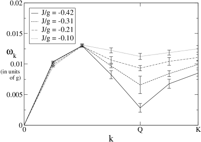
Figure 11: The dispersion $\omega_{\boldsymbol{k}}$ of the photon-like mode for different values of $J/g$. As $J/g$ approaches the critical point $(J/g)_{c}=-0.43$, the energy of the $\boldsymbol{k}=\boldsymbol{Q}$ photon goes to $0$. Thus, this critical point is an example of the class of phase transitions depicted in Fig. 10b.

Figure 12: The Brillouin zone for the honeycomb lattice. The instability to plaquette order occurs at modes (24) with wave vectors $\boldsymbol{k}=\pm\boldsymbol{Q}$.

Again, we need to include fluctuations to obtain the correct physics. Instanton fluctuations gap the photon modes, destroying the string condensation on both sides of the transition. The result is that the transition is actually a simple symmetry breaking transition -between a small string state and a plaquette crystal state (Fig. 6b).

To obtain the critical theory, note that due to the instanton fluctuations, the only low lying modes are those with $\boldsymbol{k}\approx\pm\boldsymbol{Q}$. These modes can be parameterized as

$$E_{\boldsymbol{r}\boldsymbol{s}} = \zeta(\boldsymbol{r})E_{+\boldsymbol{Q},\boldsymbol{r}\boldsymbol{s}}+\zeta^{*}(\boldsymbol{r})E_{-\boldsymbol{Q},\boldsymbol{r}\boldsymbol{s}}$$ (16)

$$A_{\boldsymbol{r}\boldsymbol{s}} = \theta(\boldsymbol{r})A_{+\boldsymbol{Q},\boldsymbol{r}\boldsymbol{s}}+\theta^{*}(\boldsymbol{r})A_{-\boldsymbol{Q},\boldsymbol{r}\boldsymbol{s}}$$ (17)

where $\zeta(\boldsymbol{r}),\theta(\boldsymbol{r})$ vary slowly on the scale of the lattice spacing. Substituting these expressions into the Lagrangian (7), and integrating out the $\theta$ field gives an action of the form

$${\cal L}=\frac{\rho}{2}\left(|\partial_{t}\zeta|^{2}-v^{2}|\partial_{x}\zeta|^{2}\right)-A|\zeta|^{2}$$ (18)

where $A\propto c_{\boldsymbol{Q}}$.

This is still not quite the correct critical theory. To get the full theory, we need to take fluctuations in $\zeta$ into account by including higher order terms. Following the analysis preceding (25), we include the most general terms consistent with the lattice symmetries:

$${\cal L}=\frac{\rho}{2}\left(|\partial_{t}\zeta|^{2}-v^{2}|\partial_{x}\zeta|^{2}\right)-A|\zeta|^{2}-B|\zeta|^{4}-C(\zeta^{6}+\text{h.c.})$$ (19)

The result is the critical theory for a $Z_{6}$ symmetry breaking transition - not surprising, given the symmetries of the two phases. At the transition, the $\zeta^{6}$ term is irrelevant and the critical point is in the universality class of the 3D $XY$ model.

We would like to mention that there is another possibility that we cannot rule out: the phase transition could be first order. Because we implemented the restricted minimization procedure described in Appendix A we cannot resolve this question. However, in principle the mean field technique can address this issue. One simply needs to use a more general minimization procedure.

V.3 Transition via instability at $\boldsymbol{k}=0$

The third type of transition - where a photon mode at $\boldsymbol{k}=0$ becomes unstable (Fig. 10a) - does not occur in the nearest neighbor XXZ spin model (I). However, with an additional second nearest neighbor interaction $J_{3}\sum_{\langle\langle\boldsymbol{i}\boldsymbol{j}\rangle\rangle}S^{z}_{\boldsymbol{i}}S^{z}_{\boldsymbol{j}}$, such a transition does occur.

With the addition of the second nearest neighbor term, the mean field phase diagram changes to the one shown in Fig. 7(a). The phase adjacent to the string condensed phase is not plaquette ordered, but instead is stripe ordered (Fig. 9) with simultaneous string condensation. The transition occurs when the $\boldsymbol{k}=0$ mode

$$E_{\boldsymbol{r}\boldsymbol{s}} = \boldsymbol{n}\cdot(\boldsymbol{s}-\boldsymbol{r})$$ (20)

$$A_{\boldsymbol{r}\boldsymbol{s}} = 0$$

becomes unstable (Fig. 13). The mean field critical theory is described by tuning the coefficient $c=\lim_{k\rightarrow 0}c_{\boldsymbol{k}}$ through $0$ in the effective Lagrangian (10).

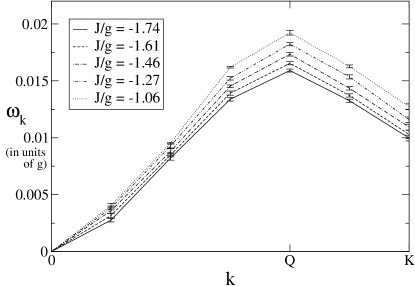
Figure 13: The dispersion $\omega_{\boldsymbol{k}}$ of the photon-like mode for different values of $J/g$ and $J_{3}/g=0.17$. As $J/g$ approaches the critical point $(J/g)_{c}=-1.83$, the velocity of the photon at $\boldsymbol{k}=0$ goes to $0$. Thus, this critical point is an example of the class of phase transitions depicted in Fig. 10a.

It is useful to rewrite this theory in real space. Since we are only interested in the low lying modes with $\boldsymbol{k}$ small, we can make the approximation $b_{\boldsymbol{k}}\approx b$, $c_{\boldsymbol{k}}\approx c+ek^{2}$, $d_{\boldsymbol{k}}\approx dk^{2}$. Going to a real space, continuum description gives a Lagrangian of the form

$${\cal L}=b^{\prime}\boldsymbol{E}\dot{\boldsymbol{A}}-c^{\prime}\boldsymbol{E}^{2}-d^{\prime}(\nabla\times\boldsymbol{A})^{2}-e^{\prime}(\nabla\times\boldsymbol{E})^{2}$$ (21)

where $b^{\prime},c^{\prime},d^{\prime},e^{\prime}$ are the renormalized continuum coefficients corresponding to $b,c,d,e$. The transition is described by tuning $c^{\prime}$ through $0$. The critical theory is thus a Rokhsar-Kivelson type theory described by a $U(1)$ gauge theory with dynamical exponent $z=2$.

The above is the mean field critical theory. In principle, we need to consider fluctuations to get the full critical theory. In particular, we need to include instanton fluctuations, replacing the $(\nabla\times\boldsymbol{A})^{2}$ term with $\cos(\nabla\times\boldsymbol{A})$. We also need to include higher order terms in $\boldsymbol{E},\boldsymbol{A}$ (which are particularly important in the stripe ($c^{\prime}<0$) phase). The most general terms consistent with the lattice symmetry are given by

$${\cal L}^{\prime}=-f^{\prime}\boldsymbol{E}^{4}-g^{\prime}((\boldsymbol{E}\cdot\boldsymbol{n}_{1})(\boldsymbol{E}\cdot\boldsymbol{n}_{2})(\boldsymbol{E}\cdot\boldsymbol{n}_{3}))^{2}+...$$ (22)

where $\boldsymbol{n}_{1},\boldsymbol{n}_{2},\boldsymbol{n}_{3}$ are unit vectors along the three lattice directions.

These fluctuations have an important effect on both phases. The instantons destroy the string condensation on both sides of transition. The result is that the transition is actually a simple $Z_{6}$ symmetry breaking transition between a small string phase and a stripe phase (Fig. 7(b)). The higher order terms ${\cal L}^{\prime}$ are also important - determining the ultimate form of the ordering in the stripe phase.

However, at the critical point, both the instantons and the higher order terms ${\cal L}^{\prime}$ are irrelevant for $e^{\prime}$ sufficiently small. The critical theory is therefore described by the simple mean field Lagrangian (21). This result follows from the analysis in LABEL:FHM0353. In that paper, the authors analyzed the $z=2$ critical point (21) in the context of a quantum dimer model on the honeycomb lattice. They found that the instanton fluctuations were irrelevant for $e^{\prime}$ sufficiently small. Moreover, they found only one relevant higher order term - a cubic term $(\boldsymbol{E}\cdot\boldsymbol{n}_{1})(\boldsymbol{E}\cdot\boldsymbol{n}_{2})(\boldsymbol{E}\cdot\boldsymbol{n}_{3})$. The same analysis can be applied in our case, but the cubic term is not allowed because of the symmetry $\boldsymbol{E}\rightarrow-\boldsymbol{E}$.

Thus, the $z=2$ critical point (21) is potentially stable (just as in the previous section, we cannot rule out the possibility of a first order phase transition). This is an example of a deconfined quantum critical point. While the two adjoining phases differ by simple $Z_{6}$ symmetry breaking, the phase transition is not captured by a Landau-Ginzburg-Wilson action. Instead, the critical theory is described by gauge fluctuations which become deconfined only at the critical point.

This deconfinement is physically reasonable - the critical point connects a liquid state of small strings to a phase with an ordered state made up of infinitely long strings. Thus it is natural that the transition point is described by a liquid state of long strings. From this picture, one might expect the same phenomenon to occur in $(3+1)D$ spin models. In that case, one would expect an entire deconfined phase between a small string phase and a striped phase.

VI Conclusion

In this paper, we have described a mean field technique for quantum string (or dimer) models. The technique can be used to estimate phase diagrams, to analyze the low energy dynamics in each of the phases, and to understand the critical points separating them.

The new mean field theory developed here is more powerful than traditional mean field approaches in that it is applicable to both string condensed phases and the usual symmetry breaking phases. Thus it can be used to study phases and phase transitions beyond Landau’s symmetry breaking paradigm. One particularly interesting application is to frustrated spin systems with emergent photon-like excitations.

We have demonstrated the approach with a simple example: the XXZ model (I) in the limit $J_{1}\gg J_{xy}\gg|J_{1}-J_{2}|$. In that limit, the low energy physics of the XXZ model is described by a quantum string model which can be studied using the mean field theory. We find that the model is in a paramagnetic phase for large positive $J/g$, in a plaquette ordered phase for large negative $J/g$, and that the phase transition is in the 3D XY universality class. We have also applied the mean field approach to the XXZ model (I) with an additional next-nearest neighbor coupling $J_{3}\sum_{\langle\langle\boldsymbol{i}\boldsymbol{j}\rangle\rangle}S^{z}_{\boldsymbol{i}}S^{z}_{\boldsymbol{j}}$. The mean field theory predicts that the model is in a paramagnetic phase for large positive $J/g$, in a stripe ordered phase for large negative $J/g$, and that the phase transition is a $z=2$ deconfined quantum critical point (21).

Given these results, it would interesting to study the XXZ model (I) numerically. A quantum Monte Carlo study could potentially access the $z=2$ deconfined quantum critical point. In addition, it could resolve the discrepancy between the resonating plaquette phase predicted by LABEL:XM0555 and the frozen plaquette phase that appears to be favored by the mean field approach (Fig. 8).

A natural direction for future research would be to apply the mean field approach to a $(3+1)$ dimensional spin model. Indeed, the mean field method may be most useful in this context. While string condensed phases with emergent photons are always unstable in $(2+1)$ dimensions, there is no such problem in $(3+1)$ dimensions. Thus, the mean field method can be used to find entire phases with string condensation and emergent photons, in addition to deconfined quantum critical points.

Appendix A Minimizing the energy

In general, the mean field phase diagram should be computed by minimizing the ground state energy $\langle H\rangle$ over all choices for $\Psi_{\{z\}}$, and then identifying the quantum phase associated with the minimum energy $\Psi_{\{z\}}$. Ideally, the minimization of $\langle H\rangle$ should be done in an unbiased fashion and include all possible $\{z\}$. However, to simplify our numerics, we have executed a more restricted minimization. In this section, we describe this minimization procedure.

In the restricted minimization procedure, we only minimize $\langle H\rangle$ over the string liquid states, $z_{\boldsymbol{i}\boldsymbol{j}}=\alpha$. We then check to make sure that the minimal $z_{\boldsymbol{i}\boldsymbol{j}}=\alpha$ state is stable to infinitesimal perturbations $\alpha\rightarrow\alpha+\delta z_{\boldsymbol{i}\boldsymbol{j}}$.

To do this, we parameterize the perturbations by $\alpha+\delta z_{\boldsymbol{i}\boldsymbol{j}}=\alpha e^{E_{\boldsymbol{i}\boldsymbol{j}}+iA_{\boldsymbol{i}\boldsymbol{j}}}$ where $E_{\boldsymbol{i}\boldsymbol{j}}$ and $A_{\boldsymbol{i}\boldsymbol{j}}$ are real - as in section IV. Expanding the energy to quadratic order in $E,A$, one finds

$$\langle H\rangle=\sum_{\boldsymbol{i}\boldsymbol{j},\boldsymbol{k}\boldsymbol{l}}(c_{\boldsymbol{i}\boldsymbol{j},\boldsymbol{k}\boldsymbol{l}}E_{\boldsymbol{i}\boldsymbol{j}}E_{\boldsymbol{k}\boldsymbol{l}}+d_{\boldsymbol{i}\boldsymbol{j},\boldsymbol{k}\boldsymbol{l}}A_{\boldsymbol{i}\boldsymbol{j}}A_{\boldsymbol{k}\boldsymbol{l}})$$ (23)

where the constants $c_{\boldsymbol{i}\boldsymbol{j},\boldsymbol{k}\boldsymbol{l}},d_{\boldsymbol{i}\boldsymbol{j},\boldsymbol{k}\boldsymbol{l}}$ are given by the equal time correlation functions (8).

To check for stability one needs to check whether the matrices $c_{\boldsymbol{i}\boldsymbol{j},\boldsymbol{k}\boldsymbol{l}},d_{\boldsymbol{i}\boldsymbol{j},\boldsymbol{k}\boldsymbol{l}}$ are positive definite. This can be accomplished most easily by going to Fourier space, where $c_{\boldsymbol{i}\boldsymbol{j},\boldsymbol{k}\boldsymbol{l}},d_{\boldsymbol{i}\boldsymbol{j},\boldsymbol{k}\boldsymbol{l}}$ are diagonal. If all of the resulting eigenvalues are positive, then the state $\Psi_{\alpha}$ is stable. Otherwise it is unstable.

If it is stable, we assume that it is the true lowest energy state. If it is unstable, say in the direction $\alpha\rightarrow\alpha e^{E_{\boldsymbol{i}\boldsymbol{j}}+iA_{\boldsymbol{i}\boldsymbol{j}}}$, we conclude that the system enters a new (symmetry breaking) phase with an ordering given by $\alpha e^{E_{\boldsymbol{i}\boldsymbol{j}}+iA_{\boldsymbol{i}\boldsymbol{j}}}$. In effect, by restricting attention to local instabilities, we assume that the phase transitions out of the liquid phases are second order or weakly first order.

This restricted minimization procedure is less powerful and less reliable then a general minimization of $\langle H\rangle$ over all $\Psi_{\{z\}}$. Its only advantage is that it is technically simpler to implement.

Appendix B Calculation of mean field phase diagram

In the following, we describe in detail how the mean field phase diagram for (3) was obtained. We begin with the transition at $J/g=0.27$. The transition at $J/g=0.27$ was obtained by calculating the optimal (minimal energy) $\alpha$ for different values of $J/g$. Plotting $\alpha$ as a function of $J/g$, we find that when $J/g$ is reduced below $0.27$, the minimum energy $\alpha$ becomes larger than $\alpha_{c}=2^{-1/4}=0.8409...$ (see Fig. 14). Thus, at this point, the variational ground state enters the string condensed phase.

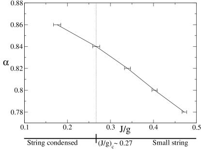
Figure 14: A plot of the minimum energy $\alpha$ as a function of $J/g$, obtained from a variational Monte Carlo simulation on a $12\times 12$ lattice. The (mean field) critical point separating the string condensed and small string phases is given by the value of $(J/g)$ where $\alpha=\alpha_{c}\approx 0.84$.

The string condensed (liquid) phase persists for $-0.43<J/g<0.27$. When $J/g<-0.43$, we find that the liquid becomes unstable (see Fig. 15). In fact, two modes become unstable simultaneously. The two unstable modes are of the form

$$E_{\boldsymbol{r}\boldsymbol{s}} = E_{\pm\boldsymbol{Q},\boldsymbol{s}\boldsymbol{r}}=\frac{1}{\sqrt{3Na^{2}}}(\boldsymbol{n}\cdot(\boldsymbol{s}-\boldsymbol{r})e^{\pm i\boldsymbol{Q}\cdot\boldsymbol{r}}$$ (24)

$$A_{\boldsymbol{r}\boldsymbol{s}} = 0$$

where $\pm Q$ are the two wave vectors shown in Fig. 12, and $\boldsymbol{n}\perp\boldsymbol{Q}$.

Because two modes become unstable simultaneously, there is an ambiguity in the way the system orders. The system could potentially order in any (real) linear combination of the two modes: $E_{\boldsymbol{r}\boldsymbol{s}}=\zeta E_{+\boldsymbol{Q},\boldsymbol{r}\boldsymbol{s}}+\zeta^{*}E_{-\boldsymbol{Q},\boldsymbol{r}\boldsymbol{s}}$.

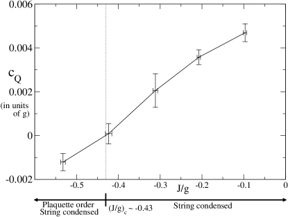
Figure 15: The eigenvalue $c_{\boldsymbol{Q}}$ corresponding to the mode (24), as a function of $(J/g)$. The liquid becomes unstable when $c_{\boldsymbol{Q}}$ becomes negative. From the above plot, we find an instability at $(J/g)_{c}\sim-0.43$.

A purely quadratic analysis cannot distinguish between this continuum of possible orderings. However, we expect that higher order terms will pick out a particular ordering. Indeed, let us consider the energy as a function of the complex parameter $\zeta$, $\langle H\rangle=H(\zeta)$. The symmetry of the lattice requires that $H(\zeta)=H(-\zeta)=H(\zeta^{*})$ and $H(\zeta)=H(\omega\zeta)$ where $\omega$ is a third root of unity. The most general form for $H$ satisfying these constraints is

$$H(\zeta)=A|\zeta|^{2}+B|\zeta|^{4}+C(\zeta^{6}+(\zeta^{*})^{6})+...$$ (25)

to sixth order in $\zeta$. The first two terms are not sensitive to the phase of $\zeta$ and therefore tell us nothing about which linear combination is favored. However, the third term does pick out a phase. The phase depends on whether $C$ is positive or negative. If $C$ is positive, imaginary $\zeta$ is favored. This corresponds to a “frozen plaquette” phase - where a third of the plaquettes are typically occupied by strings, and the interstitial bonds are likely to be empty (Fig. 8a). On the other hand, if $C$ is negative, real $\zeta$ is favored. This corresponds to a “resonating plaquette” phase where a third of the plaquettes resonate between two different configurations, while the interstitial bonds are typically occupied (Fig. 8b).

While it is difficult to determine which of these two possibilities occur using the restricted minimization procedure, one can make a determination by implementing a general minimization of $\langle H\rangle$ over all $\Psi_{\{z\}}$. We have implemented this on a $3\times 3$ lattice and the result is that the frozen plaquette phase is favored. Based on this result, we believe that $C$ is positive and the instability at $J/g=-0.43$ results in frozen plaquette order. However, a more complete numerical study is necessary to even make a definitive mean-field prediction.

When $J/g$ is decreased below $-0.43$ the system acquires (frozen) plaquette order. However, the ordering is weak near the transition point, and a finite amount of ordering is necessary to destroy string condensation. This means that the string condensation persists for a finite interval below $-0.43$ - the system enters into a phase with simultaneous plaquette order and string condensation.

We have not executed systematic numerics beyond $-0.43$. However, small lattice results suggest that plaquette order strengthens as $J/g$ decreases. This suggests that when $J/g$ becomes sufficiently large and negative, the plaquette order becomes sufficiently strong that string condensation can no longer coexist and is destroyed. The system then enters a phase with the same plaquette order but no string condensation.

The phase diagram for the model (I) with next nearest neighbor coupling $J_{3}\sum_{\langle\langle\boldsymbol{i}\boldsymbol{j}\rangle\rangle}S^{z}_{\boldsymbol{i}}S^{z}_{\boldsymbol{j}}$ was computed using the same technique. We will not repeat the details here because of their similarity to those described above.

References

- Wen (2002) X.-G. Wen, Phys. Rev. Lett. 88, 11602 (2002).
- Motrunich and Senthil (2002) O. I. Motrunich and T. Senthil, Phys. Rev. Lett. 89, 277004 (2002).
- Wen (2003) X.-G. Wen, Phys. Rev. B 68, 115413 (2003).
- Moessner and Sondhi (2003) R. Moessner and S. L. Sondhi, Phys. Rev. B 68, 184512 (2003).
- Wen (2004) X.-G. Wen, Quantum Field Theory of Many-Body Systems – From the Origin of Sound to an Origin of Light and Electrons (Oxford Univ. Press, Oxford, 2004).
- Hermele et al. (2004) M. Hermele, M. P. A. Fisher, and L. Balents, Phys. Rev. B 69, 064404 (2004).
- Levin and Wen (2005a) M. Levin and X.-G. Wen, Rev. Mod. Phys. 77, 871 (2005a).
- Levin and Wen (2005b) M. Levin and X.-G. Wen, Phys. Rev. B 71, 045110 (2005b).
- Levin and Wen (2006) M. Levin and X.-G. Wen, Phys. Rev. B 73, 035122 (2006).
- Xu and Moore (2005) C. Xu and J. E. Moore, Phys. Rev. B 72, 064455 (2005).
- Boyanovsky et al. (1980) D. Boyanovsky, R. Deza, and L. Masperi, Phys. Rev. D 22, 3034 (1980).
- Horn and Weinstein (1982) D. Horn and M. Weinstein, Phys. Rev. D 25, 3331 (1982).
- Domany et al. (1981) E. Domany, D. Mukamel, B. Nienhuis, and A. Schwimmer, Nucl. Phys. B 190, 279 (1981).
- Rokhsar and Kivelson (1988) D. S. Rokhsar and S. A. Kivelson, Phys. Rev. Lett. 61, 2376 (1988).
- Polyakov (1975) A. M. Polyakov, Phys. Lett. B 59, 82 (1975).
- Coleman and Weinberg (1973) S. Coleman and E. Weinberg, Phys. Rev. D 7, 1888 (1973).
- Halperin et al. (1974) B. I. Halperin, T. C. Lubensky, and S. K. Ma, Phys. Rev. Lett. 32, 292 (1974).
- Fradkin et al. (2004) E. Fradkin, D. A. Huse, R. Moessner, V. Oganesyan, and S. L. Sondhi, Phys. Rev. B 69, 224415 (2004).