Dichotomy in underdoped high $T_{c}$ superconductors and
spinon-dopon approach to $t$-$t^{\prime}$-$t^{\prime\prime}$-$J$ model

Abstract

We studied underdoped high $T_{c}$ superconductors using a spinon-dopon approach (or doped-carrier approach) to $t$-$t^{\prime}$-$t^{\prime\prime}$-$J$ model, where spinon carries spin and dopon carries both spin and charge. In this approach, the mixing of spinon and dopon describes superconductivity. We found that a nonuniform mixing in $k$-space is most effective in lowering the $t^{\prime}$ and $t^{\prime\prime}$ hopping energy. We showed that at mean-field level, the mixing is proportional to quasiparticle spectral weight $Z_{-}$. We also found a simple monte-carlo algorithm to calculate $Z_{-}$ from the projected spinon-dopon wavefunction, which confirms the mean-field result. Thus the non-uniform mixing caused by $t^{\prime}$ and $t"$ explains the different electron spectral weights near the nodal and anti-nodal points (i.e. the dichotomy) observed in underdoped high $T_{c}$ superconductors. For hole-doped sample, we found that $Z$ is enhanced in the nodal region and suppressed in the anti-nodal region. For electron doped sample, the same approach leads to a suppressed $Z$ in the nodal region and enhanced in the anti-nodal region, in agreement with experimental observations.

I Introduction

One powerful experimental technique to study high-$T_{c}$ material is the Angular Resolved Photoemission Spectroscopy (ARPES)Damascelli et al. (2003). ARPES study for the pseudogap region showed a strong anisotropy of the electron spectral function in momentum spaceShen and Schrieffer (1997); Zhou et al. (2004). Basically it was found that in the nodal direction, excitations are more quasi-particle like; while in the anti-nodal direction, excitations have no quasi-particle peak. This is the so-called dichotomy. If one lowers the temperature to let the material to go into superconducting phase, it was found that anti-nodal direction also has a small quasi-particle peak. Tunneling experiments show that the underdoped samples are inhomogeneousPan et al. (2001); Howald et al. (2001); McElroy et al. (2005). Due to this inhomogeneity, it is possible that the underdoped sample can be separated into optimal doped regions and underdoped regions, and the quasi-particle peak only comes from the optimal doped region. With such a point of view, it is possible that even the superconducting phase can have a very anisotropic electron spectral function in momentum space.

Exact diagonalization on $t$-$t^{\prime}$-$t^{\prime\prime}$-$J$ model ($t^{\prime}$ and $t^{\prime\prime}$ stand for next nearest neighbor and next next nearest neighbor, respectively) with 32 sites has been doneLeung and Gooding (1995); Leung et al. (1997) for hole-doped case (one hole doped). It was found that if $t^{\prime}=t^{\prime\prime}=0,J=0.3t$, then the quasiparticle weight $Z_{-}$ is almost a constant along the direction $(\pi,0)$-$(0,\pi)$: $Z_{-}=0.311$ at $(\pi/2,\pi/2)$, and $Z_{-}=0.342$ at $(\pi,0)$. However if one put in $t^{\prime}=-0.3t,t^{\prime\prime}=0.2t,J=0.3t$, which is an optimal parameter fitting for $\mbox{Sr}_{2}\mbox{CuO}_{2}\mbox{Cl}_{2}$, then there is a strong dichotomy feature: $Z_{-}=0.353$ at $(\pi/2,\pi/2)$, and $Z_{-}=0.029$ at $(\pi,0)$. This suggests that the dichotomy can be a result of $t^{\prime}$ and $t^{\prime\prime}$ hopping.

Exact diagonalization was also done for the electron doped case (a few electrons doped on 32 sites)Leung et al. (1997), where $Z_{+}$ was measured. Due to the particle-hole symmetry at half-filling, we know that if $t^{\prime}=t^{\prime\prime}=0$, $Z_{+}$ and $Z_{-}$ are equal up to a momentum shift of $(\pi,\pi)$. Therefore $Z_{+}$ are also flat along the direction $(\pi,0)$-$(0,\pi)$ in pure $t$-$J$ model. But when we put in $t^{\prime}=-0.3t,t^{\prime\prime}=0.2t,J=0.3t$, the particle-hole symmetry was broken. $Z_{+}$ was found to develop a strong anisotropy along $(\pi,0)$-$(0,\pi)$: $Z_{+}=0.005$ at $(\pi/2,\pi/2)$, and $Z_{+}=0.636$ at $(\pi,0)$.

What mechanism can destroy the quasi-particle coherence in the anti-nodal region? The simplest thing comes into one’s mind is that we need some other things to destroy it. For example, neutron scattering experiments indicate that there are some low energy magnetic fluctuationsFong et al. (1999); Tranquada et al. (1995); Aeppli et al. (1997); Yamada et al. (1998), and it was proposedShen and Schrieffer (1997); Zhou et al. (2004) that magnon scattering process can destroy the quasi-particle coherence in anti-nodal region. In this paper, however, we propose a physically different scenario: The dichotomy is due to the $t^{\prime}$ and $t^{\prime\prime}$ hopping terms. The quasiparticle spectral weight $Z_{k}$ is naturally suppressed in some region in $k$-space to lower the $t^{\prime}$ and $t"$ hopping energy. This contradicts a naive thinking that hopping always enhance $Z_{k}$. Using the $t$-$t^{\prime}$-$t^{\prime\prime}$-$J$ model, we will show that the new scenario can explain the distribution of $Z_{k}$ for both hole-doped and electron-doped samples in a unified way.

If we believe that the dichotomy is driven by the $t^{\prime}$ and $t^{\prime\prime}$ hopping terms, then there is an important issue: Is there a mean-field theory and the corresponding trial wavefunction that captures this mechanism?

One way to understand high-$T_{c}$ superconductors is to view them as doped Mott-insulators. Under Zhang-Rice singlet mappingZhang and Rice (1988), the minimal model which includes the essential Mott physics is $t$-$J$ model on square lattice. On the analytical side, a powerful mean-field theory for $t$-$J$ model, the slave-boson approach, was developedBaskaran et al. (1987); Kotliar and Liu (1988); Lee et al. (2006). This approach emphasizes the fractionalization picture of the doped Mott insulator: electron is splited into a spinon (a fermion with spin and no charge) and a holon (a boson with charge and no spin), which characterize the low energy excitations of the doped Mott insulator. This mean-field approach also successfully predicted the pseudogap metal for underdoped samples. On the numerical side, the same physics picture gives rise to the projected BCS wavefunctionGros (1988)(pBCSwf), which turns out to be a very good trial wavefunction for $t$-$J$ model. However, more detailed studies of pBCSwfNave et al. (2006); Bieri and Ivanov (2006) indicate that the slave-boson approach fail to explain the dichotomy. So a momentum dependent quasiparticle weight $Z_{k}$ remains to be a big challenge for slave-boson theory.

In this paper, we will use a new spinon-dopon approachRibeiro and Wen (2005) and the corresponding trial wavefunction to study the underdoped samples. Instead of using spinons and holons, in the new approach, we use the spinons and the bond states of spinons and holons to describe the low energy excitations. The bond states of spinons and holons are called dopons which are charge-$e$ spin-$\frac{1}{2}$ fermions. The spinon-dopon approach leads to a new trial wavefunction, the projected spinon-dopon wave function (pSDwf). The new trial wave function turns out to be an improvement over the old projected BCS wavefunction (pBCSwf).

The holon condensation in slave-boson approach correspond to spinon-dopon mixing. However, in the spinon-dopon approach, the mixing can have a momentum dependence, which is beyond the mean-field slave-boson approach. If we set the mixing to have no momentum dependence, then the pSDwf turns out to be identical to the old pBCSwf. So the pSDwf is a generalization of the pBCSwf.

Now the question is, why the mixing wants to have strong momentum dependence? The answer is that the wavefunction with momentum dependent mixing can make the hopping more coherent, and therefore gain hopping energy. Roughly speaking, the pSDwf with momentum dependent mixing is the summation of the old projected BCS wavefunction together with hopping terms $c_{i}^{\dagger}c_{j}$ acting on it. Here one should notice that the old pBCSwf, with uniform mixing, already has a pretty good $t$ hopping energy. But to have a good $t^{\prime}$ and $t^{\prime\prime}$ hopping energy, the mixing needs to have a momentum dependence, along the direction from $(\pi,0)$ to $(0,\pi)$. Our Monte Carlo calculation shows that pSDwf with momentum dependent mixing is indeed a better trial wavefunction in energetic sense. To get a quantitative sense how big is the improvement, we find that the energy of a doped hole in pSDwf is about $0.4t$ lower than that of a doped hole in pBCSwf. This is a very big improvement, indicating that the spin-charge correlation (or more precisely, the spin configuration near a doped hole) is much better described by pSDwf than pBCSwf.

Can one measure the momentum dependence of mixing? The answer is yes. In this article we will show that the mixing is directly related to $Z_{-}$, the quasi-particle weight, which is measurable in ARPES. Roughly speaking, mixing is proportional to $Z_{-}$. We have also developed a Monte Carlo technique to calculate $Z_{-}$. The calculation shows that momentum dependent mixing pSDwf indeed has strong anisotropy in momentum space, and consistent with the observed dichotomy.

Comparing pBCSwf and pSDwf, we like to point out two wave functions have similar background spin-spin correlation and similar spin energy. However, that pBCSwf does not capture the detailed charge dynamics. The new trial wavefunction, pSDwf, contains more correct spin-charge correlation. As a result, the energy of doped holes/electrons is much lower in the pSDwf. The holes/electrons in the pSDwf reproduce the correct momentum dependence of quasi-particle spectral weight. We also expect our pSDwf to have a strong momentum dependence in quasi-particle current, which may explain the temperature dependence of superfluid density of High $T_{c}$ superconductorsLiang et al. (2005).

II Spinon-dopon Approach and pSDwf

II.1 Slave-boson Approach and Projected BCS Wavefunction – Why the approach fails to capture $k$-dependent features?

Why would we want to introduce the spinon-dopon approach to $t$-$J$ model? Let us firstly look into the previous mean field approach, more specifically, slave-boson approach. The general $t$-$J$ model can be written in terms of electron operator:

$$H_{tJ}= J\sum_{\langle ij\rangle\in NN}\left(\mathbf{S}_{i}\cdot\mathbf{S}_{j}-\frac{1}{4}n_{i}n_{j}\right)$$

$$-\sum_{ij}t_{ij}\mathbf{P}\left(c_{i}^{\dagger}c_{j}+c_{j}^{\dagger}c_{i}\right)\mathbf{P}.$$ (1)

Here the projection operator $\mathbf{P}$ is to ensure the Hamiltonian is acting within the physical Hilbert space: one each site, the physical states are $|\uparrow\rangle$, $|\downarrow\rangle$ or $|0\rangle$, i.e., no double occupancy.

Slave-boson approachBaskaran et al. (1987); Kotliar and Liu (1988) emphasizes the spin-charge separation picture. In that approach, one splits electron operator into spinon and holon operators:

$$c_{i\sigma}=f_{i\sigma}b_{i}^{\dagger},$$ (2)

where $f$ is spinon, carrying spin $1/2$ and charge $0$, $i$ labels site and $\sigma$ labels spin; $b$ is holon, carrying spin $0$ and charge $1$. This splitting enlarges the Hilbert space. To go back to physical Hilbert space, a local constraint is needed:

$$f_{i\uparrow}^{\dagger}f_{i\uparrow}+f_{i\downarrow}^{\dagger}f_{i\downarrow}+b_{i}^{\dagger}b_{i}=1.$$ (3)

Due to spin interaction, spinons form a $d$-wave paired state. The superconducting phase is realized through an additional holon condensation at momentum $k=0$. Within such a construction, the quasi-particle weight $Z$ is proportional to doping $x$ everywhere in k-space, in both nodal and anti-nodal region. To see this, one can simply look at the mean-field Green function of electron:

$$\langle c_{k}c^{\dagger}_{k}\rangle=\langle b^{\dagger}_{k=0}b_{k=0}f_{k}f^{\dagger}_{k}\rangle=x\langle f_{k}f^{\dagger}_{k}\rangle.$$ (4)

Therefore $x$ is the residue of quasi-particle pole and $Z=x$ is independent of $k$.

Slave-boson approach is supposed to capture the physics of spin-charge separation. It has successfully generated the phase diagram of High-$T_{c}$ superconductor. But this approach, at least at mean-field level, could not capture some more detailed features, such as momentum dependence of quasi-particle weight or the quasi-particle current. One can argue that including gauge fluctuation, those detailed features may be reproduced, but here we will try to develop another approach which can capture these features at mean-field level.

Before we go into the new spinon-dopon approach, let us see how far one can go using slave-boson approach. One can actually try to build a trial wavefunction based on slave-boson mean-field approach. We know that the mean-field approach enlarged the Hilbert space, and the resulting wavefunction lies outside the physical Hilbert space. Only when one includes the full gauge fluctuations can one go back to the physical Hilbert space.

So one way to include the full gauge fluctuations, is to build the mean-field ground state first, and then do a projection from the enlarged Hilbert space to the physical Hilbert space. The wavefunction after projection would serve as a trial wavefunction for the physical Hamiltonian. This projected wavefunction is supposed to incorporate the effect of gauge fluctuation of the slave-boson approach, and may answer the question that, after including gauge fluctuation, whether slave-boson approach can capture the detailed features like dichotomy.

The mean-field ground state for underdoped case can be constructed as follows. Let $N_{h}$ be the number of holes, $N_{f}$ is the number of spinons, and $N=N_{h}+N_{f}$ is the total number of sites. The slave-boson mean-field ground state is then given by

$$|\Phi_{SB,mean}\rangle=(b_{k=0}^{\dagger})^{N_{h}}\prod_{k}(u_{k}+v_{k}f_{k\uparrow}^{\dagger}f_{-k\downarrow}^{\dagger})|0\rangle,$$ (5)

where the spinon part of the wavefunction is a standard $d$-wave pairing state:

$$\frac{v_{k}}{u_{k}}=\frac{\Delta(k)}{\xi_{k}+\sqrt{\xi_{k}^{2}+\Delta(k)^{2}}},$$ (6)

where

$$\xi_{k} =-2\chi(\cos k_{x}+\cos k_{y})-\mu$$

$$\Delta(k) =\Delta(\cos k_{x}-\cos k_{y}) \mbox{(d-wave)}.$$ (7)

Here $\mu$ is the chemical potential to give the correct average number of spinon $\langle\sum_{i}f_{i\sigma}^{\dagger}f_{i\sigma}\rangle=N_{f}$; $\chi$ and $\Delta$ are mean-field parameters which have been found to be $\frac{\Delta}{\chi}=2$ Lee and Nagaosa (1992) at half-filling, and $\frac{\Delta}{\chi}$ decreases to zero at doping around $J/t$.

Now one can do a projection to go back to the physical Hilbert space. The constraint for physical Hilbert space is Eq.(3). This constraint ensures that the total number of spinon must be $N_{f}$ and there is no double occupancy of spinon: spinon number $n_{f,i}$ at site $i$ has to be either 0 or 1. One can easily see that the resulting wavefunction is the usual Projected $d$-wave BCS Wavefunction (pBCSwf):

$$|\Phi_{PBCS}\rangle =P_{D}^{SB}P_{N}^{SB}|\Phi_{SB,mean}\rangle$$ (8)

$$=P_{D}P_{N}\prod_{k}(u_{k}+v_{k}c_{k\uparrow}^{\dagger}c_{-k\downarrow}^{\dagger})|0\rangle$$ (9)

$$\propto P_{D}\left(\sum_{k}a(k)c_{k\uparrow}^{\dagger}c_{-k\downarrow}^{\dagger}\right)^{N_{f}/2}|0\rangle,$$ (10)

where in the first line, $P_{N}^{SB}$ is the projection into fixed total number of particles, i.e., $N_{h}$ holons and $N_{f}$ spinons; while $P_{D}^{SB}$ is the projection into physical Hilbert space, i.e., removing all states not satisfying constraint Eq.(3). In the second line, $P_{N}$ is the projection into fixed total number of electrons, which has to be $N_{f}$, $P_{D}$ is the projection which removes all double occupancies. $a(k)$ is defined as $a(k)=\frac{v_{k}}{u_{k}}$.

Projected BSC wavefunction turned out to be a surprisingly good trial wavefunction for $t$-$J$ modelGros (1988). However numerical studiesNave et al. (2006); Bieri and Ivanov (2006) showed that the quasi-particle weight is almost a constant along the direction from $(\pi,0)$ to $(0,\pi)$, i.e., it fails to reproduce the dichotomy. The quasi-particle current of pBCSwf is also pretty smooth in the $k$ spaceNave et al. (2006). It is because pBCSwf is unable to capture the momentum dependence properties that we need a new approach to underdoped high $T_{c}$ superconductors.

II.2 How to capture $k$-dependence features?
– Spinon-dopon approach and projected spinon-dopon wavefunction

Rebeiro and WenRibeiro and Wen (2005) developed this new mean-field approach trying to capture the spinon-holon recombination physics. In the following we briefly review their work. We know that at low temperature, spinon and holon recombine pretty strongly to give electron-like quasi-particle. So it is natural to introduce dopon operator – a bound state between a spinon and a holon – to describe low energy excitations. Note that a dopon has the same quantum number as an electron and describes a doped electron (or hole). But the Mott and spin-liquid physics at half filling should also be addressed. So one should also keep the spinon operator. As a result, two types of fermions are introduced here: spinon $f$ and dopon $d$. Spinon carries spin $1/2$ and no charge, and dopon carries spin $1/2$ and charge $1$. By introducing these two types of fermions one enlarges the Hilbert space: now there are 16 states per site, among them only three are physical. The three physical states on site $i$ can be represented in terms of spinon and dopon fermions as:

$$|\uparrow\rangle=|\uparrow_{f}\rangle, |\downarrow\rangle=|\downarrow_{f}\rangle, |0\rangle=\frac{1}{\sqrt{2}}|\uparrow_{f}\downarrow_{d}-\downarrow_{f}\uparrow_{d}\rangle.$$ (11)

Here please notice that the constraints are two-fold: firstly there must be one $f$ spinon per site, secondly $d$ dopon has to form a local singlet with the spinon.

One can do a self-consistent mean-field study. The mean-field Hamiltonian takes the form:

$$H_{mean} =(-2\chi(\cos k_{x}+\cos k_{y})-\mu)f_{k\alpha}^{\dagger}f_{k\alpha}$$

$$+\Delta(\cos k_{x}-\cos k_{y})f_{k\uparrow}^{\dagger}f_{-k\downarrow}^{\dagger}+\epsilon_{k}d_{k\alpha}^{\dagger}d_{k\alpha}$$

$$+\beta_{k}f_{k\alpha}^{\dagger}d_{k\alpha}+h.c..$$ (12)

Here $H_{mean}$ can be divided into three parts: spinon part, dopon part and spinon-dopon interaction. The spinon part describes the usual $d$-wave paired ansatz: $\chi=J\langle f_{k\alpha}^{\dagger}f_{k\alpha}\rangle$, $\Delta=J\langle f_{k\uparrow}f_{-k\downarrow}\rangle$. The dopon part is simply a free dopon band, with $\epsilon_{k}$ determined by high energy ARPES measurement. Note that $\epsilon_{k}$ is not taken as tunable mean-field parameter. Finally the spinon-dopon interaction is described by a $k$-dependent hybridization, roughly speaking $\beta_{k}=\epsilon_{k}\langle d_{i}^{\dagger}f_{i}\rangle$. One can see that $d_{i}^{\dagger}f_{i}$ is a bosonic field carrying charge $1$ and spin $0$. Its non-zero average value corresponds to holon condensation in slave-boson approach, which leads to superconductivity. $\mu$ is the chemical potential required to tune the doping.

Along this line Rebeiro and Wen did a mean-field phase diagram, and successfully fit to ARPES data and tunneling dataRibeiro and Wen (2006a, b). Here we try to emphasize that the main lesson we learned from this new mean-field approach is that one can have a $k$-dependent hybridization at mean-field level (in Eq.(12) this hybridization is controlled by $\beta_{k}$ and energy spectrum of spinon band and dopon band.), which is roughly the counterpart of holon condensation in slave-boson approach. This is why one can study detailed features like dichotomy in this new approach.

Several open questions naturally arise in this new approach. It seems there are two types of excitations, spinon and dopon, what do they look like? We also know that mean-field approach is not very reliable, so it would be nice to understand the physical trial wavefunction corresponding to the new mean-field approach, from where we would know exactly what we are doing. In the following we try to answer these questions.

Let us construct trial wavefunctions based on this spinon-dopon mean-field approach. One can simply take a mean-field ground state wavefunction, then do a projection back into the physical Hilbert space, just like the way we did in the slave boson case:

$$|\Phi_{PSD}\rangle=P_{SD}P_{N}|\Phi_{SD,mean}\rangle.$$ (13)

Here $P_{N}$ is the projection into fixed number of spinon and dopon, which gives the correct doping; and $P_{SD}$ is the projection into to physical Hilbert space Eq.(11). $|\Phi_{SD,mean}\rangle$ is the ground state wavefunction of some mean-field Hamiltonian in the form of Eq.(12). Suppose we know how to do this projection numerically, one can do a variational study of the these Projected Spinon-Dopon Wavefunctions (pSDwf), to see what is the lowest-energy ansatz. In general, however, the full projection is not doable, so we develop a simple numerical technique to do a local projection to have some rough idea about what kind of wavefunction is energetically favorable (See Appendix A). What we found is that the best trial wavefunction for underdoped case has the following form:

$$|\Phi_{PSD}^{SC}\rangle =P_{SD}P_{N}|\Phi_{SD,mean}^{SC}\rangle$$ (14)

$$=P_{SD}P_{N}\exp\left(\sum_{k}b(k)\tilde{f}_{k\uparrow}^{\dagger}\tilde{f}_{-k\downarrow}^{\dagger}\right)|0\rangle$$ (15)

$$\propto P_{SD}\left(\sum_{k}b(k)\tilde{f}_{k\uparrow}^{\dagger}\tilde{f}_{-k\downarrow}^{\dagger}\right)^{\frac{N+N_{h}}{2}}|0\rangle,$$ (16)

where

$$\tilde{f}^{\dagger}_{k\alpha}=\sqrt{1-\beta_{k}^{2}}f_{k\alpha}^{\dagger}+\beta_{k}d_{k\alpha}^{\dagger}.$$ (17)

Here $\tilde{f}$ form a $d$-wave paired state and the superscript $SC$ means this wavefunction is superconducting. $b(k)$ and $\beta_{k}$ are some real functions and we assume $\beta_{k}=\beta_{-k}$ to respect time reversal symmetry. For this particular ansatz, full projection is doable in low doping limit. In section IV we develop the numerical method to do the full projection and we will see that this wavefunction is a even better trial wavefunction than pBCSwf.

Note that the total number of $f$ and $d$ fermions is $N+N_{h}$. Also $P_{SD}$ requires one $f$-fermion per site, so totally $N$ $f$-fermions. Therefore we must have $N_{h}$ $d$-fermions, which gives the correct doping.

II.3 How does pSDwf capture the $k$-dependent features? – properties of wavefunction before projection $|\Phi_{SD,mean}^{SC}\rangle$: $Z_{k}$ at mean-field level.

The form of $|\Phi_{PSD}^{SC}\rangle$ looks very similar to pBCSwf, basically we are constructing a pairing wavefunction based on hybridized fermion $\tilde{f}_{k}$. In the next section we will see that $|\Phi_{PSD}^{SC}\rangle$ and pBCSwf are indeed closely related. For the moment let us have a closer look at the wavefunction $|\Phi_{SD,mean}^{SC}\rangle$ before projection. The idea is that physical properties may not change drastically after the projection. In this case the mean-field level understanding will give us insight of the wavefunction after the projection.

First of all it is obvious that this wavefunction is superconducting. That is because the nonzero $\beta_{k}$ signals the mixing between spinon and dopon $\langle f_{k\alpha}^{\dagger}d_{k\alpha}\rangle\neq 0$, and thus signals breaking of charge conservation. It is natural to believe the superconductivity survives after projection.

Let us introduce the other combination of $f$ and $d$ fermions:

$$\tilde{d}^{\dagger}_{k\alpha}=-\beta_{k}f_{k\alpha}^{\dagger}+\sqrt{1-\beta_{k}^{2}}d_{k\alpha}^{\dagger},$$ (18)

and the quasi-particle operators:

$$\gamma_{k\uparrow}^{\dagger} =\tilde{u}_{k}\tilde{f}_{k\uparrow}^{\dagger}-\tilde{v}_{k}\tilde{f}_{-k\downarrow}$$ (19)

$$\gamma_{-k\downarrow} =\tilde{u}_{k}\tilde{f}_{-k\downarrow}+\tilde{v}_{k}\tilde{f}_{k\uparrow}^{\dagger},$$ (20)

where

$$\tilde{u}_{k}=\frac{1}{\sqrt{1+b(k)^{2}}} \tilde{v}_{k}=\frac{b(k)}{\sqrt{1+b(k)^{2}}},$$ (21)

are the coherent factors for a $d$-wave paired state. We can show that

$$|\Phi_{SD,mean}^{SC}\rangle=\exp\left(\sum_{k}b(k)\tilde{f}_{k\uparrow}^{\dagger}\tilde{f}_{-k\downarrow}^{\dagger}\right)|0\rangle,$$

satisfies:

$$\tilde{d}_{k\alpha}|\Phi_{SD,mean}^{SC}\rangle=0,$$ (22)

and

$$\gamma_{k\alpha}|\Phi_{SD,mean}^{SC}\rangle=0.$$ (23)

The mean-field Hamiltonian which can generate $|\Phi_{SD,mean}^{SC}\rangle$ as ground state is simply:

$$H_{mean}=\sum_{k}\left(\epsilon_{\tilde{f}}(k)\gamma_{k\alpha}^{\dagger}\gamma_{-k\alpha}+\epsilon_{\tilde{d}}(k)\tilde{d}_{k\alpha}^{\dagger}\tilde{d}_{k\alpha}\right),$$ (24)

with $\epsilon_{\tilde{f}}(k),\epsilon_{\tilde{d}}(k)\geqslant 0$. Later we will see that there are physical reasons that $\epsilon_{\tilde{d}}(k)>\epsilon_{\tilde{f}}(k)$, meaning $\tilde{f}$ band is lowest energy excitation, and $\tilde{d}$ band is fully gapped, $\epsilon_{\tilde{d}}(k)>0$ for any $k$.

We can express $f$ and $d$ fermions in terms of $\gamma$ and $\tilde{d}$ fermions:

$$f_{k\alpha} =\sqrt{1-\beta_{k}^{2}}(\tilde{u}_{k}\gamma_{k\alpha}+\tilde{v}_{k}\epsilon_{\alpha\delta}\gamma_{-k\delta}^{\dagger})-\beta_{k}\tilde{d}_{k\alpha}$$ (25)

$$d_{k\alpha} =\beta_{k}(\tilde{u}_{k}\gamma_{k\alpha}+\tilde{v}_{k}\epsilon_{\alpha\delta}\gamma_{-k\delta}^{\dagger})+\sqrt{1-\beta_{k}^{2}}\tilde{d}_{k\alpha}.$$ (26)

Based on Eq.(25) and (26), it is easy to obtain:

$$\frac{\langle\Phi_{SD,mean}^{SC}|f_{k\alpha}^{\dagger}f_{k\alpha}|\Phi_{SD,mean}^{SC}\rangle}{\langle\Phi_{SD,mean}^{SC}||\Phi_{SD,mean}^{SC}\rangle} =(1-\beta_{k}^{2})\tilde{v}_{k}^{2}$$ (27)

$$\frac{\langle\Phi_{SD,mean}^{SC}|d_{k\alpha}^{\dagger}d_{k\alpha}|\Phi_{SD,mean}^{SC}\rangle}{\langle\Phi_{SD,mean}^{SC}||\Phi_{SD,mean}^{SC}\rangle} =\beta_{k}^{2}\tilde{v}_{k}^{2}.$$ (28)

We know that the mean-field wavefunction should give one $f$-fermion and $x=\frac{N_{h}}{N}$ $d$-fermion per site on average:

$$\sum_{k}(1-\beta_{k}^{2})\tilde{v}_{k}^{2} =N$$ (29)

$$\sum_{k}\beta_{k}^{2}\tilde{v}_{k}^{2} =N_{h}$$ (30)

In the low doping limit $x\rightarrow 0$, it is clear from the above relations that $\beta_{k}^{2}\propto x$.

Now let us understand how to calculate $Z_{-}$ and $Z_{+}$ on this mean-field wavefunction. $Z_{+}$ and $Z_{-}$ are defined to be:

$$Z_{-,k} =\frac{|\langle N-1,k|c_{k}|\Phi_{GS}^{N}\rangle|^{2}}{\langle N-1,k|N-1,k\rangle\langle\Phi_{GS}^{N}|\Phi_{GS}^{N}\rangle},$$ (31)

$$Z_{+,k} =\frac{|\langle N+1,k|c_{k}^{\dagger}|\Phi_{GS}^{N}\rangle|^{2}}{\langle N+1,k|N+1,k\rangle\langle\Phi_{GS}^{N}|\Phi_{GS}^{N}\rangle},$$ (32)

where $|N-1,k\rangle$ ($|N+1,k\rangle$) are the lowest-energy $N-1$ ($N+1$) electron states which have nonzero overlap with $c_{k}|\Phi_{GS}^{N}\rangle$ ($c_{k}^{\dagger}|\Phi_{GS}^{N}\rangle$).

In our mean-field wavefunction, the lowerest energy excited states are given by creating $\gamma_{k}$-quasi-particle. Note that now $d_{k}^{\dagger}$ is the hole creation operator, so at mean-field level the $Z_{k}$ for spinon-dopon wavefunction are:

$$Z_{-,k\uparrow}^{SD} ={\textstyle\frac{|\langle\Phi_{SD,mean}^{SC}|\gamma_{k\uparrow}d_{k\uparrow}^{\dagger}|\Phi_{SD,mean}^{SC}\rangle|^{2}}{\langle\Phi_{SD,mean}^{SC}|\gamma_{k\uparrow}\gamma_{k\uparrow}^{\dagger}|\Phi_{SD,mean}^{SC}\rangle\langle\Phi_{SD,mean}^{SC}|\Phi_{SD,mean}^{SC}\rangle}},$$

$$=\beta_{k}^{2}\tilde{u}_{k}^{2}$$ (33)

$$Z_{+,k\uparrow}^{SD} ={\textstyle\frac{|\langle\Phi_{SD,mean}^{SC}|\gamma_{-k\downarrow}d_{k\uparrow}|\Phi_{SD,mean}^{SC}\rangle|^{2}}{\langle\Phi_{SD,mean}^{SC}|\gamma_{-k\downarrow}\gamma_{-k\downarrow}^{\dagger}|\Phi_{SD,mean}^{SC}\rangle\langle\Phi_{SD,mean}^{SC}|\Phi_{SD,mean}^{SC}\rangle}}$$

$$=\beta_{k}^{2}\tilde{v}_{k}^{2}.$$ (34)

At this moment, let us compare spinon-dopon wavefunction (SDwf) with BCS wavefunction (BCSwf), both before projection (In Section II.4 we will compare them after projection).

In Section II.1 we view pBCSwf as the projected slave-boson mean-field state into physical Hilbert space. We may also view pBCSwf as projected BCSwf with all double occupancies removed:

$$|\Phi_{PBCS}\rangle =P_{D}P_{N}|\Phi_{BCS}\rangle$$ (35)

$$=P_{D}P_{N}\exp(\sum_{k}a(k)c_{k\uparrow}^{\dagger}c_{-k\downarrow}^{\dagger})|0\rangle$$ (36)

$$\propto P_{D}\left(\sum_{k}a(k)c_{k\uparrow}^{\dagger}c_{-k\downarrow}^{\dagger}\right)^{N_{f}/2}|0\rangle,$$ (37)

where

$$|\Phi_{BCS}\rangle =\exp(\sum_{k}a(k)c_{k\uparrow}^{\dagger}c_{-k\downarrow}^{\dagger})|0\rangle$$ (38)

$$\propto\prod_{k}(u_{k}+v_{k}c_{k\uparrow}^{\dagger}c_{-k\downarrow}^{\dagger})|0\rangle.$$ (39)

Before the projection, the spectral weight of the electron operator $c_{k}$ can be calculated easily:

$$Z_{-,k}^{BCS}=v_{k}^{2}=n_{k} Z_{+,k}^{BCS}=u_{k}^{2}=1-n_{k},$$ (40)

where $n_{k}=\langle c_{k}^{\dagger}c_{k}\rangle_{BCS}$. For a $d$-wave BCSwf Eq.(6), we can plot the $Z_{k}$ in Fig.1. In low doping limit, parameters are taken as $\mu=0$, $\chi=1$, $\Delta=0.55$. Such choice of parameters leads to a pBCSwf with lowest average energy at half filling.

    

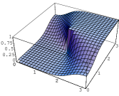
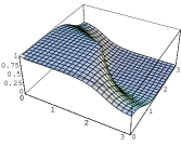
Figure 1: Plot of $u_{k}^{2}$ (left) and $v_{k}^{2}$ (right) within one quarter Brillouin Zone, $k_{x}$ and $k_{y}$ range from $0$ to $\pi$.

The $Z_{+,k}$ and $Z_{-,k}$ for the pBCSwf after the projection were also calculatedNave et al. (2006). Roughly speaking what was found is that the $Z_{k}$ profile after projection is similar to that before the projection. There is a quasi fermi surface, which is roughly along the diagonal direction, $Z_{-,k}$ is large inside the fermi surface and decreases very fast when you go outside fermi surface; while $Z_{+,k}$ is large outside fermi surface, and decreases fast when you go into fermi surface. But there is one big difference, which is a reduction factor. For the $Z_{+,k}$, this reduction factor was found to be proportional to $x$. But for $Z_{-,k}$, this reduction factor depends on $k$ and is finite (around $0.2$) for $k=(0,0)$ even at low-doping limit. From slave-boson approach Eq.(4), we already see that $Z\propto x$ at mean field level. Basically at half filling, $Z=0$ and we have a Mott insulator instead of a band insulator.

Notice that along diagonal direction $(\pi,0)-(0,\pi)$, the $Z_{k}^{BCS}$ is dispersionless: $Z_{k}^{BCS}=0.5$, which does not have dichotomy feature; After projection, there is a factor $x$ reduction, but $Z_{k}$ is still almost a constant along the diagonal directionBieri and Ivanov (2006); Nave et al. (2006).

To compare the calculated $Z$ from the BSCwf and SDwf, we note that the projected wave functions, pBCSwf and pSDwf, are closely related (see section II.4). More precisely:

$$|\Phi_{PSD}^{SC}\rangle=|\Phi_{PBCS}\rangle\mbox{ if:}$$

$$\tilde{u}_{k}=v_{k},\; \tilde{v}_{k}=u_{k},\mbox{ and }\beta_{k}=\beta_{0}\mbox{ (constant)}$$ (41)

It is easy to understand this identification at half-filling, since both wavefunctions simply give the same spin-liquid (usually referred to as staggered flux spin liquid in literatures), characterized by $\chi$ and $\Delta$. Now in the pSDwf $\tilde{f}=f$, with no mixing with $d$-fermion. It is simply a particle-hole transformed pBCSwf, by which $u_{k}$ transformed into $\tilde{v}_{k}$ and vice versa. The important message is that $u_{k},v_{k}$ and $\tilde{u}_{k},\tilde{v}_{k}$ characterize the spin dynamics, but $\beta_{k}$ characterizes the charge dynamics.

With this identification in mind, from Eq.(33,34) and (40) we immediately know that when $\beta_{k}=\beta_{0}$ these two wavefunctions give the same mean-field $Z_{k}$ profile except that SDwf has an extra $x$ factor, because $\beta_{k}^{2}=\beta_{0}^{2}\propto x$ in low doping limit. However, when $\beta_{k}$ has a strong $k$-dependence, $Z_{k}$ from the two approaches can be very different.

Let us think about whether or not these wavefunctions can capture dichotomy in low doping limit. What did we learn from these mean-field result? We learned that it is impossible to capture dichotomy by BCSwf, because in order to capture the $k$-dependence along $(0,\pi)$–$(\pi,0)$, one has to tune $u_{k},\ v_{k}$. Because $d$-wave $u_{k},v_{k}$ are constant along $(0,\pi)$–$(\pi,0)$, one has to destroy the $d$-wave ansatz to have a $k$-dependent $u_{k},\ v_{k}$ along $(0,\pi)$–$(\pi,0)$. This leads to a higher $J$ energy. On the other hand, it is possible to capture dichotomy by SDwf, because one can tune $\beta_{k}$ to have a strong $k$-dependence while keeping $\tilde{u}_{k},\tilde{v}_{k}$ to be $d$-wave ansatz. This will not destroy the spin background. Based on our experience of projection, we expect that even after projection, the above statement is qualitatively true.

II.4 Why mixing $\beta_{k}$ has a strong $k$-dependence? –Relation between pBCSwf and pSDwf

In the last section we see that pSDwf can potentially capture the dichotomy through a $k$ dependent $\beta_{k}$. Now the issue is, why does the $\beta_{k}$ want to have a $k$ dependence that can explain the dichotomy in $Z_{k}$? Why does such $k$-dependent $\beta_{k}$ lead to a pSDwf which is energetically more favorable? To understand this, we need to know what a pSDwf looks like in real space.

The discussion below for identifying the relation between pSDwf and pBCSwf is rather long. The result, however, is simple. Let us present the result here first. We introduce $\tilde{\beta}_{k}=\beta_{k}/\sqrt{1-\beta_{k}^{2}}$. In low doping limit, $\tilde{\beta}_{k}\approx\beta_{k}$. For the simplest one-hole case, if $\tilde{\beta}_{k}$ has the simplest modulation in $k$-space $\tilde{\beta}_{k}=\tilde{\beta}_{0}+2\tilde{\beta}_{1}(\cos k_{x}+\cos k_{y})$, then the pSDwf can be viewed as pBCSwf mixed with the wavefunction generated by the nearest neighbor hopping operators (see Eq.(68)). For more complicated $\tilde{\beta}_{k}=\tilde{\beta}_{0}+2\tilde{\beta}_{1}(\cos k_{x}+\cos k_{y})+4\tilde{\beta}_{2}\cos k_{x}\cos k_{y}+2\tilde{\beta}_{3}(\cos 2k_{x}+\cos 2k_{y})$, the pSDwf can be viewed as pBCSwf mixed with the wavefunction generated by the nearest neighbor, next nearest neighbor and third nearest neighbor hopping operators (see Eq.(75)). Therefore to lower the hopping energy, finite $\beta_{i}$’s are naturally developed. This is why $\beta_{k}$ with a proper $k$ dependence is more energetically favorable.

Before we look into pSDwf, let us review what a pBCSwf looks like in real space. One can do a Fourier transformation:

$$|\Phi_{PBCS}\rangle=P_{D}\left(\sum_{k}a(k)c_{k\uparrow}^{\dagger}c_{-k\downarrow}^{\dagger}\right)^{N_{f}/2}|0\rangle=P_{D}\left(\sum_{\mathbf{R}_{i\uparrow},\mathbf{R}_{j\downarrow}}a(\mathbf{R}_{j\downarrow}-\mathbf{R}_{i\uparrow})c_{\mathbf{R}_{i\uparrow},\uparrow}^{\dagger}c_{\mathbf{R}_{j\downarrow},\downarrow}^{\dagger}\right)^{N_{f}/2}|0\rangle,$$ (42)

where $a(\mathbf{r})=\sum_{k}a(k)\cos(k\cdot\mathbf{r})$. If we have a spin basis $\{\mathbf{R}_{i\uparrow},\mathbf{R}_{j\downarrow}\}$, where $\mathbf{R}_{i\uparrow}$ labels the positions of spin up electrons and $\mathbf{R}_{j\downarrow}$ labels the positions of spin down electrons:

$$\langle\{\mathbf{R}_{i\uparrow},\mathbf{R}_{j\downarrow}\}|\Phi_{PBCS}\rangle=\left|\begin{array}[]{cccc}a(\mathbf{R}_{1\downarrow}-\mathbf{R}_{1\uparrow})&a(\mathbf{R}_{1\downarrow}-\mathbf{R}_{2\uparrow})&\cdots&a(\mathbf{R}_{1\downarrow}-\mathbf{R}_{\frac{N_{f}}{2}\uparrow})\\ a(\mathbf{R}_{2\downarrow}-\mathbf{R}_{1\uparrow})&a(\mathbf{R}_{2\downarrow}-\mathbf{R}_{2\uparrow})&\cdots&a(\mathbf{R}_{2\downarrow}-\mathbf{R}_{\frac{N_{f}}{2}\uparrow})\\ \vdots&\vdots&\ddots&\vdots\\ a(\mathbf{R}_{\frac{N_{f}}{2}\downarrow}-\mathbf{R}_{1\uparrow})&a(\mathbf{R}_{\frac{N_{f}}{2}\downarrow}-\mathbf{R}_{2\uparrow})&\cdots&a(\mathbf{R}_{\frac{N_{f}}{2}\downarrow}-\mathbf{R}_{\frac{N_{f}}{2}\uparrow})\end{array}\right|.$$ (47)

We see that the overlap between a spin basis and pBCSwf is simply a single slater determinant of a two-particle wavefunction. This is why pBCSwf can be numerically simulated on a fairly large lattice.

Now we go back to pSDwf. Up to a normalization constant, one can express pSDwf as:

$$|\Phi_{PSD}^{SC}\rangle=P_{SD}\left(\sum_{k}b(k)(f_{k\uparrow}^{\dagger}+\tilde{\beta}_{k}d_{k\uparrow}^{\dagger})(f_{-k\downarrow}^{\dagger}+\tilde{\beta}_{k}d_{-k\downarrow}^{\dagger})\right)^{\frac{N+N_{h}}{2}}|0\rangle$$ (48)

where $\tilde{\beta}_{k}=\beta_{k}/\sqrt{1-\beta_{k}^{2}}$. Since $\beta_{k}\propto\sqrt{x}$, in the low doping limit, $\tilde{\beta}_{k}=\beta_{k}$.

One can also do a Fourier transformation into the real space:

$$|\Phi_{PSD}^{SC}\rangle=P_{SD}\left(\sum_{\mathbf{R}_{i\uparrow},\mathbf{R}_{j\downarrow}}b(\mathbf{R}_{j\downarrow}-\mathbf{R}_{i\uparrow})(f_{\mathbf{R}_{i\uparrow}\uparrow}^{\dagger}+\tilde{\beta}_{0}d_{\mathbf{R}_{i\uparrow}\uparrow}^{\dagger}+\sum_{\mathbf{\delta}}\tilde{\beta}_{\delta}d_{\mathbf{R}_{i\uparrow}+\mathbf{\delta},\uparrow}^{\dagger})(f_{\mathbf{R}_{j\downarrow}\downarrow}^{\dagger}+\tilde{\beta}_{0}d_{\mathbf{R}_{j\downarrow}\downarrow}^{\dagger}+\sum_{\mathbf{\delta}}\tilde{\beta}_{\delta}d_{\mathbf{R}_{j\downarrow}+\mathbf{\delta},\downarrow}^{\dagger})\right)^{\frac{N+N_{h}}{2}}|0\rangle,$$ (49)

where $\tilde{\beta}_{\mathbf{\delta}}$’s are the Fourier components of $\tilde{\beta}_{k}$:

$$\tilde{\beta}_{k}=\tilde{\beta}_{0}+\tilde{\beta}_{\mathbf{x}}e^{ik_{x}}+\tilde{\beta}_{-\mathbf{x}}e^{-ik_{x}}+\tilde{\beta}_{\mathbf{y}}e^{ik_{y}}+\tilde{\beta}_{-\mathbf{y}}e^{-ik_{y}}+\cdots.$$ (50)

We should only consider the rotation invariant $\tilde{\beta}_{k}$, and let us only keep the first three Fourier components:

$$\tilde{\beta}_{k}= \tilde{\beta}_{0}+2\tilde{\beta}_{1}(\cos k_{x}+\cos k_{y})+4\tilde{\beta}_{2}\cos k_{x}\cos k_{y}$$

$$+2\tilde{\beta}_{3}(\cos 2k_{x}+\cos 2k_{y}).$$ (51)

We claimed that if $\tilde{\beta}_{k}=\tilde{\beta}_{0}$, then pSDwf is identical to pBCSwf if $b(k)=\frac{1}{a(k)}$. Let us see how that is true. Without $\beta_{1,2,3}$, Eq.(49) is:

$$|\Phi_{PSD}^{SC}(\tilde{\beta}_{0})\rangle=P_{SD}\left(\sum_{\mathbf{R}_{i\uparrow},\mathbf{R}_{j\downarrow}}b(\mathbf{R}_{j\downarrow}-\mathbf{R}_{i\uparrow})(f_{\mathbf{R}_{i\uparrow}\uparrow}^{\dagger}+\tilde{\beta}_{0}d_{\mathbf{R}_{i\uparrow}\uparrow}^{\dagger})(f_{\mathbf{R}_{j\downarrow}\downarrow}^{\dagger}+\tilde{\beta}_{0}d_{\mathbf{R}_{j\downarrow}\downarrow}^{\dagger})\right)^{\frac{N+N_{h}}{2}}|0\rangle.$$ (52)

What does a pBCSwf look like? If one does a particle-hole transformation $c_{i\uparrow}^{\dagger}\rightarrow h_{i\downarrow}$, pBCSwf is:

$$|\Phi_{PBCS}\rangle=P_{D}\left(\sum_{k}\frac{1}{a(k)}h_{k\uparrow}^{\dagger}h_{-k\downarrow}^{\dagger}\right)^{\frac{N+N_{h}}{2}}|0\rangle$$ (53)

$$=P_{D}\left(\sum_{\mathbf{R}_{i\uparrow},\mathbf{R}_{j\downarrow}}b(\mathbf{R}_{j\downarrow}-\mathbf{R}_{i\uparrow})h_{\mathbf{R}_{i\uparrow},\uparrow}^{\dagger}h_{\mathbf{R}_{j\downarrow},\downarrow}^{\dagger}\right)^{\frac{N+N_{h}}{2}}|0\rangle,$$ (54)

where $P_{D}$ is the projection forbidding any empty site.

If we consider a spin basis $\{\mathbf{R}_{i\uparrow},\mathbf{R}_{j\downarrow}\}$, with the empty sites $\{\mathbf{R}_{k,0}\}$, then after particle-hole transformation, we have single occupied sites $\{\mathbf{R}_{i\uparrow},\mathbf{R}_{j\downarrow}\}$, and double occupied sites $\{\mathbf{R}_{k,0}\}$. So the position of spin up and down sites in the hole representation are $\{\mathbf{\tilde{R}}_{i\uparrow},\mathbf{\tilde{R}}_{j\downarrow}\}_{h}$, where $\{\mathbf{\tilde{R}}_{i\uparrow}\}_{h}=\{\mathbf{R}_{i\uparrow}\}\cup\{\mathbf{R}_{k,0}\}$ and $\{\mathbf{\tilde{R}}_{j\downarrow}\}_{h}=\{\mathbf{R}_{j\downarrow}\}\cup\{\mathbf{R}_{k,0}\}$. The overlap of pBCSwf and the spin basis in hole representation is:

$$\langle\{\mathbf{R}_{i\uparrow},\mathbf{R}_{j\downarrow}\}|\Phi_{PBCS}\rangle=\langle\{\mathbf{\tilde{R}}_{i\uparrow},\mathbf{\tilde{R}}_{j\downarrow}\}_{h}|\Phi_{PBCS}\rangle$$

$$= \left|\begin{array}[]{cccc}b(\mathbf{\tilde{R}}_{1\downarrow}-\mathbf{\tilde{R}}_{1\uparrow})&b(\mathbf{\tilde{R}}_{1\downarrow}-\mathbf{\tilde{R}}_{2\uparrow})&\cdots&b(\mathbf{\tilde{R}}_{1\downarrow}-\mathbf{\tilde{R}}_{\frac{N+N_{h}}{2}\uparrow})\\ b(\mathbf{\tilde{R}}_{2\downarrow}-\mathbf{\tilde{R}}_{1\uparrow})&b(\mathbf{\tilde{R}}_{2\downarrow}-\mathbf{\tilde{R}}_{2\uparrow})&\cdots&b(\mathbf{\tilde{R}}_{2\downarrow}-\mathbf{\tilde{R}}_{\frac{N+N_{h}}{2}\uparrow})\\ \vdots&\vdots&\ddots&\vdots\\ b(\mathbf{\tilde{R}}_{\frac{N+N_{h}}{2}\downarrow}-\mathbf{\tilde{R}}_{1\uparrow})&b(\mathbf{\tilde{R}}_{\frac{N+N_{h}}{2}\downarrow}-\mathbf{\tilde{R}}_{2\uparrow})&\cdots&b(\mathbf{\tilde{R}}_{\frac{N+N_{h}}{2}\downarrow}-\mathbf{\tilde{R}}_{\frac{N+N_{h}}{2}\uparrow})\end{array}\right|.$$ (59)

The equation works this way because if one simply expands the polynomial in Eq.(54), each sum will give you one term in the expansion of the determinant in Eq.(59), and Pauli statistics is accounted by the sign in determinant expansion.

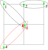
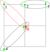
Figure 2: pSDwf with only $\tilde{\beta}_{0}$. The site $0$ is empty. $f$-fermions are represented by green spin, and $d$-fermion is represented by red spin. Black valence bonds are bonds with of $f$-fermions, while red valence bond has a $d$-fermion. The two figures are two contributions of the overlap between pSDwf and a spin basis $|1_{\uparrow}3_{\uparrow}2_{\downarrow}4_{\downarrow}0_{emp}\rangle$, and they correspond to the same term in determinant Eq.(64). The two figures give rise to states: $\mbox{left: }|\uparrow_{1f}\downarrow_{0f}\uparrow_{3f}\downarrow_{2f}\uparrow_{0d}\downarrow_{4f}\rangle=|\uparrow_{1f}\uparrow_{3f}\downarrow_{2f}\downarrow_{4f}(\downarrow_{0f}\uparrow_{0d})\rangle$ and $\mbox{right: }|\uparrow_{1f}\downarrow_{0d}\uparrow_{3f}\downarrow_{2f}\uparrow_{0f}\downarrow_{4f}\rangle=-|\uparrow_{1f}\uparrow_{3f}\downarrow_{2f}\downarrow_{4f}(\uparrow_{0f}\downarrow_{0d})\rangle$ The minus sign means that the two figures contribute additively.

Now we can do the same analysis on pSDwf Eq.(52). First of all $\tilde{\beta}_{0}$ is not relevant in the wavefunction, since we are projecting into a state with fixed number of $d$-fermion, which means that all $\tilde{\beta}_{0}$ does is to give an overall factor $\tilde{\beta}_{0}^{N_{h}}$ in front of the wavefunction. To have an overlap with spin basis $\{\mathbf{R}_{i\uparrow},\mathbf{R}_{j\downarrow},\mathbf{R}_{k,0}\}$, we know that on empty site $\mathbf{R}_{k,0}$ the expansion of polynomial Eq.(52) should give either $|\uparrow_{f}\downarrow_{d}\rangle$ or $|\uparrow_{d}\downarrow_{f}\rangle$. After projection each case would contribute to $\frac{1}{\sqrt{2}}|0\rangle$ where $|0\rangle=\frac{1}{\sqrt{2}}(|\uparrow_{f}\downarrow_{d}\rangle+|\uparrow_{d}\downarrow_{f}\rangle)$

One immediately sees that the expansion of polynomial Eq.(52) gives similar terms as the expansion of Eq.(54); actually corresponding to one term in determinant Eq.(59), we have $2^{N_{h}}$ terms from Eq.(52), since we can either have $|\uparrow_{f}\downarrow_{d}\rangle$ or $|\uparrow_{d}\downarrow_{f}\rangle$ for each empty site. The details are visualized in Fig.2. Taking into account the factor$\frac{1}{\sqrt{2}}$ of projection, one has:

$$\langle\{\mathbf{R}_{i\uparrow},\mathbf{R}_{j\downarrow}\}|\Phi_{PSD}^{SC}(\tilde{\beta}_{0})\rangle= (\sqrt{2}\tilde{\beta}_{0})^{N_{h}}\left|\begin{array}[]{cccc}b(\mathbf{\tilde{R}}_{1\downarrow}-\mathbf{\tilde{R}}_{1\uparrow})&b(\mathbf{\tilde{R}}_{1\downarrow}-\mathbf{\tilde{R}}_{2\uparrow})&\cdots&b(\mathbf{\tilde{R}}_{1\downarrow}-\mathbf{\tilde{R}}_{\frac{N+N_{h}}{2}\uparrow})\\ b(\mathbf{\tilde{R}}_{2\downarrow}-\mathbf{\tilde{R}}_{1\uparrow})&b(\mathbf{\tilde{R}}_{2\downarrow}-\mathbf{\tilde{R}}_{2\uparrow})&\cdots&b(\mathbf{\tilde{R}}_{2\downarrow}-\mathbf{\tilde{R}}_{\frac{N+N_{h}}{2}\uparrow})\\ \vdots&\vdots&\ddots&\vdots\\ b(\mathbf{\tilde{R}}_{\frac{N+N_{h}}{2}\downarrow}-\mathbf{\tilde{R}}_{1\uparrow})&b(\mathbf{\tilde{R}}_{\frac{N+N_{h}}{2}\downarrow}-\mathbf{\tilde{R}}_{2\uparrow})&\cdots&b(\mathbf{\tilde{R}}_{\frac{N+N_{h}}{2}\downarrow}-\mathbf{\tilde{R}}_{\frac{N+N_{h}}{2}\uparrow})\end{array}\right|,$$ (64)

we found that $|\Phi_{PBCS}\rangle$ and $|\Phi_{PSD}^{SC}(\tilde{\beta}_{0})\rangle$ are the same wavefunction.

Now let us put in the simplest $k$-dependence in $\tilde{\beta}_{k}$:

$$\tilde{\beta}_{k}=\tilde{\beta}_{0}+2\tilde{\beta}_{1}(\cos k_{x}+\cos k_{y}),$$ (65)

we try to write $|\Phi_{PSD}^{SC}(\tilde{\beta}_{0},\tilde{\beta}_{1})\rangle$ in real space. After the Fourier transformation into real space:

$$|\Phi_{PSD}^{SC}(\tilde{\beta}_{0},\tilde{\beta}_{1})\rangle$$

$$= P_{SD}\left(\sum_{\mathbf{R}_{i\uparrow},\mathbf{R}_{j\downarrow}}b(\mathbf{R}_{j\downarrow}-\mathbf{R}_{i\uparrow})(f_{\mathbf{R}_{i\uparrow}\uparrow}^{\dagger}+\tilde{\beta}_{0}d_{\mathbf{R}_{i\uparrow}\uparrow}^{\dagger}+\tilde{\beta}_{1}\sum_{\mathbf{\delta}=\pm\hat{x},\pm\hat{y}}d_{\mathbf{R}_{i\uparrow+\mathbf{\delta}},\uparrow}^{\dagger})(f_{\mathbf{R}_{j\downarrow}\downarrow}^{\dagger}+\tilde{\beta}_{0}d_{\mathbf{R}_{j\downarrow}\downarrow}^{\dagger}+\tilde{\beta}_{1}\sum_{\mathbf{\delta}=\pm\hat{x},\pm\hat{y}}d_{\mathbf{R}_{j\downarrow+\mathbf{\delta}},\downarrow}^{\dagger})\right)^{\frac{N+N_{h}}{2}}|0\rangle.$$ (66)

If we expand this polynomial Eq.(66), of course we will still have contribution from $\tilde{\beta}_{0}$ terms which is nothing but the right hand side of Eq.(64). But apart from that, we also have contribution from $\tilde{\beta}_{1}$, which makes the problem more complicated. To start, let us consider the case of a single hole $N_{h}=1$. To have an overlap with spin basis $\{\mathbf{R}_{i\uparrow},\mathbf{R}_{j\downarrow},\mathbf{R}_{k,0}\}$, the $d$-fermion on empty site $\mathbf{R}_{k,0}$ can also come from a bond connecting a spinful site and $\mathbf{R}_{k,0}+\mathbf{\delta}$, which is the $\tilde{\beta}_{1}$ term effect. Let us consider the case $\mathbf{\delta}=\hat{y}$. We can also assume the spin state on site $\mathbf{R}_{k,0}+\mathbf{\delta}$ is spin down. Now it appears that we have two ways to construct the empty site on $\mathbf{R}_{k,0}$: $|\uparrow_{f}\downarrow_{d}\rangle$ or $|\uparrow_{d}\downarrow_{f}\rangle$. We study the two cases separately. Firstly if the empty site is constructed by $|\uparrow_{f}\downarrow_{d}\rangle$, shown in Fig.3, careful observation tells us that the contribution to the overlap is exactly cancelled by fermion statistics. On the other hand, if the empty site is constructed by $|\uparrow_{d}\downarrow_{f}\rangle$, we have the case in Fig.4. After careful observation, we know that this type of contribution is $-\frac{\tilde{\beta}_{1}}{2\tilde{\beta}_{0}}$ times the overlap between $|\Phi_{PSD}^{SC}(\tilde{\beta}_{0})\rangle$ and the spin basis that differs from $\{\mathbf{R}_{i\uparrow},\mathbf{R}_{j\downarrow},\mathbf{R}_{k,0}\}$ by a hopping along $\hat{y}$. Considering the fact that the shift can also be $-\hat{y}$ and $\pm\hat{x}$, one has:

$$\langle\{\mathbf{R}_{i\uparrow},\mathbf{R}_{j\downarrow},\mathbf{R}_{k,0}\}|\Phi_{PSD}^{SC}(\tilde{\beta}_{0},\tilde{\beta}_{1})\rangle$$

$$= \sqrt{2}\tilde{\beta}_{0}\langle\{\mathbf{R}_{i\uparrow},\mathbf{R}_{j\downarrow},\mathbf{R}_{k,0}\}|\Phi_{PBCS}\rangle+\left(\frac{-\tilde{\beta}_{1}}{\sqrt{2}}\right)\langle\{\mathbf{R}_{i\uparrow},\mathbf{R}_{j\downarrow},\mathbf{R}_{k,0}\}|\sum_{\mathbf{\delta}=\pm\hat{x},\pm\hat{y}}c_{\mathbf{R}_{k,0}+\mathbf{\delta},\alpha}^{\dagger}c_{\mathbf{R}_{k,0},\alpha}|\Phi_{PBCS}\rangle,$$ (67)

where the minus sign in the second terms comes from Fermi statistics.

Just by looking at Eq.(67), we arrive at the conclusion:

$$|\Phi_{PSD}^{SC}(\tilde{\beta}_{0},\tilde{\beta}_{1})\rangle=|\Phi_{PBCS}\rangle+\left(\frac{-\tilde{\beta}_{1}}{2\tilde{\beta}_{0}}\right)P_{D}\sum_{i,\mathbf{\delta}=\pm\hat{x},\pm\hat{y}}c_{i+\mathbf{\delta},\alpha}^{\dagger}c_{i,\alpha}|\Phi_{PBCS}\rangle.$$ (68)

Let us study Eq.(67). With out $\tilde{\beta}_{1}$, one has a single Slater determinant for the overlap with a spin basis; with $\tilde{\beta}_{1}$, we have $1+n_{shift}=5$ Slater determinants, where $n_{shift}$ is the total number of ways that one hole can hop. Later we will see that for $n_{h}$ holes, the number of Slater determinants for the overlap is $(1+n_{shift})^{n_{h}}$, which means numerically one can only do few holes.

The result (68) is obtained by studying one-hole case, and it is not hard to generalize the result for the multi-hole case. Basically, each hole may either not hop or hop once with a prefactor $\frac{-\tilde{\beta}_{1}}{2\tilde{\beta}_{0}}$, but not hop more than once. For example, for two-hole case, we have:

$$|\Phi_{PSD}^{SC}(\tilde{\beta}_{0},\tilde{\beta}_{1})\rangle=\left(1+P_{D}\sum_{i,\mathbf{\delta}=\pm\hat{x},\pm\hat{y}}\frac{-\tilde{\beta}_{1}}{2\tilde{\beta}_{0}}c_{i+\mathbf{\delta},\alpha}^{\dagger}c_{i,\alpha}+P_{D}\frac{1}{2!}\sum_{\begin{array}[]{c}{\scriptstyle\mathbf{\delta_{1}},\mathbf{\delta_{2}}=\pm\hat{x},\pm\hat{y}}\\ {\scriptstyle j,i\neq j+\mathbf{\delta_{2}}}\end{array}}\left(\frac{-\tilde{\beta}_{1}}{2\tilde{\beta}_{0}}\right)^{2}c_{j+\mathbf{\delta_{2}},\alpha_{2}}^{\dagger}c_{j,\alpha_{2}}c_{i+\mathbf{\delta_{1}},\alpha_{1}}^{\dagger}c_{i,\alpha_{1}}\right)|\Phi_{PBCS}\rangle,$$ (71)

where the constraint $i\neq j+\mathbf{\delta_{2}}$ makes sure no hole can hop twice, and the coefficient $\frac{1}{2!}$ comes from double counting.

We can also easily generalize it to the case with $\tilde{\beta}_{2}$ and $\tilde{\beta}_{3}$…. For two hole case, we have:

$$|\Phi_{PSD}^{SC}(\tilde{\beta}_{0},\tilde{\beta}_{\mathbf{\delta}})\rangle=\left(1+P_{D}\sum_{i,\mathbf{\delta}}\frac{-\tilde{\beta}_{\mathbf{\delta}}}{2\tilde{\beta}_{0}}c_{i+\mathbf{\delta},\alpha}^{\dagger}c_{i,\alpha}+P_{D}\frac{1}{2!}\sum_{\begin{array}[]{c}{\scriptstyle\mathbf{\delta_{1}},\mathbf{\delta_{2}}}\\ {\scriptstyle j,i\neq j+\mathbf{\delta_{2}}}\end{array}}\left(\frac{-\tilde{\beta}_{\mathbf{\delta_{1}}}}{2\tilde{\beta}_{0}}\right)\left(\frac{-\tilde{\beta}_{\mathbf{\delta_{2}}}}{2\tilde{\beta}_{0}}\right)c_{j+\mathbf{\delta_{2}},\alpha_{2}}^{\dagger}c_{j,\alpha_{2}}c_{i+\mathbf{\delta_{1}},\alpha_{1}}^{\dagger}c_{i,\alpha_{1}}\right)|\Phi_{PBCS}\rangle.$$ (74)

In the end, the general formula for multi-hole pSDwf is:

$$|\Phi_{PSD}^{SC}(\tilde{\beta}_{0},\tilde{\beta}_{\mathbf{\delta}})\rangle=P_{D}\exp_{n_{hop}=0,1}{\left(1+\sum_{i,\mathbf{\delta}}\frac{-\tilde{\beta}_{\mathbf{\delta}}}{2\tilde{\beta}_{0}}c_{i+\mathbf{\delta},\alpha}^{\dagger}c_{i,\alpha}\right)}|\Phi_{PBCS}\rangle,$$ (75)

where $n_{hop}=0,1$ ensures that no hole can hop twice.

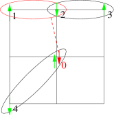
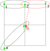
Figure 3: pSDwf with only $\tilde{\beta}_{1}$. The site $0$ is empty. $f$-fermions are represented by green spin, and $d$-fermion is represented by red spin. Black valence bonds are bonds with of $f$-fermions, while red valence bond has a $d$-fermion. Notice that the position of $d$-fermion is shifted by $-\hat{y}$ by $\tilde{\beta}_{1}$ term effect (red dotted line). The two figures show the two contributions of the overlap between pSDwf and spin basis $|1_{\uparrow}3_{\uparrow}2_{\downarrow}4_{\downarrow}0_{emp}\rangle$, with spin of $f$-fermion on site 2 and spin of $d$-fermion on site 0 are parallel. They give rise to states: $\mbox{left: }|\uparrow_{1f}\downarrow_{0d}\uparrow_{3f}\downarrow_{2f}\uparrow_{0f}\downarrow_{4f}\rangle=|\uparrow_{1f}\uparrow_{3f}\downarrow_{2f}\downarrow_{4f}(\downarrow_{0d}\uparrow_{0f})\rangle$ and $\mbox{right: }|\uparrow_{1f}\downarrow_{2f}\uparrow_{3f}\downarrow_{0d}\uparrow_{0f}\downarrow_{4f}\rangle=-|\uparrow_{1f}\uparrow_{3f}\downarrow_{2f}\downarrow_{4f}(\downarrow_{0d}\uparrow_{0f})\rangle$ The minus sign means the two figures contribute subtractively, i.e., they cancel exactly.

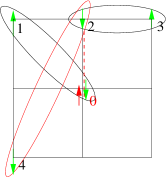
Figure 4: pSDwf with only $\tilde{\beta}_{1}$. The site $0$ is empty. $f$-fermions are represented by green spin, and $d$-fermion is represented by red spin. Black valence bonds are bonds with of $f$-fermions, while red valence bond has a $d$-fermion. Note that the position of $d$-fermion is shifted by $-\hat{y}$ by $\tilde{\beta}_{1}$ term effect (red dotted line). This figure shows another contribution to the overlap between pSDwf and spin basis $|1_{\uparrow}3_{\uparrow}2_{\downarrow}4_{\downarrow}0_{emp}\rangle$, with spin of $f$-fermion on site 2 and spin of $d$-fermion on site 0 are anti-parallel.. It gives rise to state: $|\uparrow_{1f}\downarrow_{0f}\uparrow_{3f}\downarrow_{2f}\uparrow_{0d}\downarrow_{4f}\rangle=-|\uparrow_{1f}\uparrow_{3f}\downarrow_{2f}\downarrow_{4f}(\uparrow_{0d}\downarrow_{0f})\rangle$. Note that there is a contribution for $\langle 1_{\uparrow}3_{\uparrow}0_{\downarrow}4_{\downarrow}2_{emp}|\Phi_{PSD}^{SC}(\tilde{\beta}_{0})\rangle$, with the same valence bond map, where $|1_{\uparrow}3_{\uparrow}0_{\downarrow}4_{\downarrow}2_{emp}\rangle$ is the result state after a hopping along $\hat{y}$ acting on original state $|1_{\uparrow}3_{\uparrow}2_{\downarrow}4_{\downarrow}0_{emp}\rangle$. That one would give a state $|\uparrow_{1f}\downarrow_{0f}\uparrow_{3f}\downarrow_{2f}\uparrow_{2d}\downarrow_{4f}\rangle=|\uparrow_{1f}\uparrow_{3f}\downarrow_{0f}\downarrow_{4f}(\uparrow_{2d}\downarrow_{2f})\rangle$. The minus sign in the shifted $d$-fermion overlap comes from fermi statistics.

III How to measure the mixing $\beta_{k}$? –Physical Meaning of spinon excitation and dopon excitation

From Eq.(34,33), we know what at the mean-field level, $\beta_{k}$ can be measured by spectral weight $Z$. After projection, it is natural to expect that $Z$ is also closely related to $\beta_{k}$. But how to calculate $Z$ after projection? Basically through Eq.(32,31), we need a good trial ground state and excited state. The ground state would be nothing but pSDwf. What is a good excited state? To be specific, let us study $Z_{-}$, then the question is how to obtain $|N-1\rangle$?

In pBCSwf, the good excited state (referred as quasi-particle state) is found to be:

$$|N-1\rangle_{qp}^{PBCS}=P_{D}c_{p}P_{N}|BCS\rangle,$$ (76)

where $P_{N}$ project into fixed $N_{f}$ number of electrons. The way we construct excited state here is simple: first find a excited state on the mean-field level, then do a projection. In pSDwf, which includes pBCSwf as a limit, we should have a similar formula. But now we have two possible ways to construct excitation states, since on mean-field level we have two types of fermions $f$ and $d$, they correspond to two types of excitations. Now it is important to understand what each type of excitations looks like. It turns out that the $f$-type excitation corresponds to the quasi-particle excitation, and $d$-type excitation corresponds to bare hole excitation. Thus the quasi-particle state $|N-1\rangle$ for calculating $Z_{-}$ is the $f$-type excitation.

The main result for this section is Eq.(99,100) for $f$-excitation and Eq.(109) for $d$-excitation. One can see that the $f$-excitation of pSDwf is just the quasi-particle excitation in pBCSwf together with hopping terms acting on it. And $d$-excitation is the bare hole on a pSDwf ground state. Let’s see how those happen:

For $f$-excitation,

$$|N-1\rangle_{f}=P_{SD}f_{-p}^{\dagger}P_{N}|\Phi_{SD}^{SC}\rangle$$ (77)

$$=P_{SD}f_{-p}^{\dagger}\left(\sum_{k}b(k)(f_{k\uparrow}^{\dagger}+\tilde{\beta}_{k}d_{k\uparrow}^{\dagger})(f_{-k\downarrow}^{\dagger}+\tilde{\beta}_{k}d_{-k\downarrow}^{\dagger})\right)^{\frac{N+N_{h}}{2}}|0\rangle.$$

Here $|N-1\rangle_{f}$ has $N_{f}-1$ number of electrons, because before projection there are totally $N+N_{h}+1$ fermions, and we know projection enforces one $f$-fermion per site, so totally there are $N_{h}+1$ $d$-fermions, i.e., holes. What does this wavefunction look like after projection?

To understand this we first try to understand the excitation of pBCSwf. What is the excited state in terms of spin basis? One way to see it is to identify:

$$|N-1\rangle_{qp}^{PBCS} =P_{D}c_{p\uparrow}\left(\sum_{k}a(k)c_{k\uparrow}^{\dagger}c_{-k\downarrow}^{\dagger}\right)^{N_{f}/2}|0\rangle$$ (78)

$$\propto P_{D}c_{-p\downarrow}^{\dagger}\left(\sum_{k}a(k)c_{k\uparrow}^{\dagger}c_{-k\downarrow}^{\dagger}\right)^{N_{f}/2-1}|0\rangle.$$ (79)

In this form the overlap with a spin basis $\{\mathbf{R}_{i\uparrow},\mathbf{R}_{j\downarrow}\}$ is easy to see. Notice now the number of up spins is $N_{f}/2-1$, and the number of down spins is $N_{f}/2$, so there is one more site in $\{\mathbf{R}_{j\downarrow}\}$. The only fashion to construct a spin basis is: let $c_{-p\downarrow}^{\dagger}$ create an electron somewhere, then let $a(k)c_{k\uparrow}^{\dagger}c_{-k\downarrow}^{\dagger}$ create the valence bonds. After observation, the overlap is:

$$\langle\{\mathbf{R}_{i\uparrow},\mathbf{R}_{j\downarrow}\}|N-1\rangle_{qp}^{PBCS}=\left|\begin{array}[]{ccccc}a(\mathbf{R}_{1\downarrow}-\mathbf{R}_{1\uparrow})&a(\mathbf{R}_{1\downarrow}-\mathbf{R}_{2\uparrow})&\cdots&a(\mathbf{R}_{1\downarrow}-\mathbf{R}_{\frac{N_{f}}{2}-1,\uparrow})&e^{-ip\mathbf{R}_{1\downarrow}}\\ a(\mathbf{R}_{2\downarrow}-\mathbf{R}_{1\uparrow})&a(\mathbf{R}_{2\downarrow}-\mathbf{R}_{2\uparrow})&\cdots&a(\mathbf{R}_{2\downarrow}-\mathbf{R}_{\frac{N_{f}}{2}-1,\uparrow})&e^{-ip\mathbf{R}_{2\downarrow}}\\ \vdots&\vdots&\ddots&\vdots\\ a(\mathbf{R}_{\frac{N_{f}}{2}\downarrow}-\mathbf{R}_{1\uparrow})&a(\mathbf{R}_{\frac{N_{f}}{2}\downarrow}-\mathbf{R}_{2\uparrow})&\cdots&a(\mathbf{R}_{\frac{N_{f}}{2}\downarrow}-\mathbf{R}_{\frac{N_{f}}{2}-1\uparrow})&e^{-ip\mathbf{R}_{\frac{N_{f}}{2}\downarrow}}\end{array}\right|.$$ (84)

But to compare with pSDwf formalism, we want to see the same result in a different way. Let us do a particle-hole transformation, just like what we did in Eq.(54).

$$|N-1\rangle_{qp}^{PBCS}=P_{D}c_{p\uparrow}\left(\sum_{k}a(k)c_{k\uparrow}^{\dagger}c_{-k\downarrow}^{\dagger}\right)^{N_{f}/2}|0\rangle\propto P_{D}h_{-p\downarrow}^{\dagger}\left(\sum_{k}b(k)h_{k\uparrow}^{\dagger}h_{-k\downarrow}^{\dagger}\right)^{(N+N_{h})/2}|0\rangle.$$ (85)

The only way to construct a spin basis in hole representation $\{\mathbf{\tilde{R}}_{i\uparrow},\mathbf{\tilde{R}}_{j\downarrow}\}_{h}$ is to let $h_{-p\downarrow}^{\dagger}$ construct a hole somewhere, and let $b(k)h_{k\uparrow}^{\dagger}h_{-k\downarrow}^{\dagger}$ construct the valence bonds to fill the lattice. The overlap in hole representation is:

$$\langle\{\mathbf{R}_{i\uparrow},\mathbf{R}_{j\downarrow}\}|N-1\rangle_{qp}^{PBCS}=\langle\{\mathbf{\tilde{R}}_{i\uparrow},\mathbf{\tilde{R}}_{j\downarrow}\}_{h}|N-1\rangle_{qp}^{PBCS}$$

$$= \left|\begin{array}[]{ccccc}b(\mathbf{\tilde{R}}_{1\downarrow}-\mathbf{\tilde{R}}_{1\uparrow})&b(\mathbf{\tilde{R}}_{1\downarrow}-\mathbf{\tilde{R}}_{2\uparrow})&\cdots&b(\mathbf{\tilde{R}}_{1\downarrow}-\mathbf{\tilde{R}}_{\frac{N+N_{h}}{2}\uparrow})&e^{-ip\mathbf{\tilde{R}}_{1\downarrow}}\\ b(\mathbf{\tilde{R}}_{2\downarrow}-\mathbf{\tilde{R}}_{1\uparrow})&b(\mathbf{\tilde{R}}_{2\downarrow}-\mathbf{\tilde{R}}_{2\uparrow})&\cdots&b(\mathbf{\tilde{R}}_{2\downarrow}-\mathbf{\tilde{R}}_{\frac{N+N_{h}}{2}\uparrow})&e^{-ip\mathbf{\tilde{R}}_{2\downarrow}}\\ \vdots&\vdots&\ddots&\vdots\\ b(\mathbf{\tilde{R}}_{\frac{N+N_{h}}{2}+1\downarrow}-\mathbf{\tilde{R}}_{1\uparrow})&b(\mathbf{\tilde{R}}_{\frac{N+N_{h}}{2}+1,\downarrow}-\mathbf{\tilde{R}}_{2\uparrow})&\cdots&b(\mathbf{\tilde{R}}_{\frac{N+N_{h}}{2}+1,\downarrow}-\mathbf{\tilde{R}}_{\frac{N+N_{h}}{2}\uparrow})&e^{-ip\mathbf{\tilde{R}}_{\frac{N+N_{h}}{2}+1,\downarrow}}\end{array}\right|.$$ (90)

Now let us go back to pSDwf. What is an $f$-type excitation? The only way to construct a spin basis, $|\{\mathbf{\tilde{R}}_{i\uparrow},\mathbf{\tilde{R}}_{j\downarrow}\}_{h}\rangle$, is to let $f_{-p}^{\dagger}$ construct an $f$-fermion somewhere, then let $b(k)(f_{k\uparrow}^{\dagger}+\tilde{\beta}_{k}d_{k\uparrow}^{\dagger})(f_{-k\downarrow}^{\dagger}+\tilde{\beta}_{k}d_{-k\downarrow}^{\dagger})$ construct the valence bonds to fill the whole lattice. We first consider the case $\tilde{\beta}_{k}=\tilde{\beta}_{0}$. In this case, the constructing precess is in exactly the same fashion as in Eq.(90), except for one difference: there is a coefficient of $\sqrt{2}\tilde{\beta}_{0}$ for each hole. That is because for each hole there are two contributions, one from $|\uparrow_{f}\downarrow_{d}\rangle$, the other from $|\uparrow_{d}\downarrow_{f}\rangle$, each with coefficient of $\sqrt{1/2}\tilde{\beta}_{0}$; unless that the hole and the spinon created by $f_{-p}^{\dagger}$ are on the same site, in which case we have only one contribution. If we ignore the last effect (since it is an infinitesimal change to the wavefunction in the low doping limit, and it also comes as an artifact of our projective construction), we conclude that:

$$\langle\{\mathbf{R}_{i\uparrow},\mathbf{R}_{j\downarrow}\}|N-1,\tilde{\beta}_{0}\rangle_{f}=\langle\{\mathbf{\tilde{R}}_{i\uparrow},\mathbf{\tilde{R}}_{j\downarrow}\}_{h}|N-1,\tilde{\beta}_{0}\rangle_{f}$$ (91)

$$= (\sqrt{2}\beta_{0})^{N_{h}+1}\left|\begin{array}[]{ccccc}b(\mathbf{\tilde{R}}_{1\downarrow}-\mathbf{\tilde{R}}_{1\uparrow})&b(\mathbf{\tilde{R}}_{1\downarrow}-\mathbf{\tilde{R}}_{2\uparrow})&\cdots&b(\mathbf{\tilde{R}}_{1\downarrow}-\mathbf{\tilde{R}}_{\frac{N+N_{h}}{2}\uparrow})&e^{-ip\mathbf{\tilde{R}}_{1\downarrow}}\\ b(\mathbf{\tilde{R}}_{2\downarrow}-\mathbf{\tilde{R}}_{1\uparrow})&b(\mathbf{\tilde{R}}_{2\downarrow}-\mathbf{\tilde{R}}_{2\uparrow})&\cdots&b(\mathbf{\tilde{R}}_{2\downarrow}-\mathbf{\tilde{R}}_{\frac{N+N_{h}}{2}\uparrow})&e^{-ip\mathbf{\tilde{R}}_{2\downarrow}}\\ \vdots&\vdots&\ddots&\vdots\\ b(\mathbf{\tilde{R}}_{\frac{N+N_{h}}{2}+1\downarrow}-\mathbf{\tilde{R}}_{1\uparrow})&b(\mathbf{\tilde{R}}_{\frac{N+N_{h}}{2}+1,\downarrow}-\mathbf{\tilde{R}}_{2\uparrow})&\cdots&b(\mathbf{\tilde{R}}_{\frac{N+N_{h}}{2}+1,\downarrow}-\mathbf{\tilde{R}}_{\frac{N+N_{h}}{2}\uparrow})&e^{-ip\mathbf{\tilde{R}}_{\frac{N+N_{h}}{2}+1,\downarrow}}\end{array}\right|$$ (96)

$$=(\sqrt{2}\beta_{0})^{N_{h}+1}\langle\{\mathbf{R}_{i\uparrow},\mathbf{R}_{j\downarrow}\}|N-1\rangle_{qp}^{PBCS},$$ (97)

so

$$|N-1,\tilde{\beta}_{0}\rangle_{f}\propto|N-1\rangle_{qp}^{PBCS}.$$ (98)

The point is that $f$-type excitation describes the spin-charge separation picture of the excitation, because the hole and the unpaired spinon created by $f_{-p}^{\dagger}$ can be arbitrarily separated. And it turns out to be the low energy excitation of $t$-$J$ model.

What if the mixing $\beta_{k}$ has momentum dependence? Similar to our study for the ground state wavefunction leading to Eq.(67,68), one can convince oneself that, in the one hole case

$$|N-1,\tilde{\beta}_{0},\tilde{\beta}_{1},\tilde{\beta}_{2},\tilde{\beta}_{3}\rangle_{f}\propto|N-1\rangle_{qp}^{PBCS}+\left(\frac{-\tilde{\beta}_{1}}{2\tilde{\beta}_{0}}\right)P_{D}\sum_{i,\mathbf{\delta}=\pm\hat{x},\pm\hat{y}}c_{i+\mathbf{\delta},\alpha}^{\dagger}c_{i,\alpha}|N-1\rangle_{qp}^{PBCS}$$

$$+\left(\frac{-\tilde{\beta}_{2}}{2\tilde{\beta}_{0}}\right)P_{D}\sum_{i,\mathbf{\delta}=\pm(\hat{x}+\hat{y}),\pm(\hat{x}-\hat{y})}c_{i+\mathbf{\delta},\alpha}^{\dagger}c_{i,\alpha}|N-1\rangle_{qp}^{PBCS}+\left(\frac{-\tilde{\beta}_{3}}{2\tilde{\beta}_{0}}\right)P_{D}\sum_{i,\mathbf{\delta}=\pm 2\hat{x},\pm 2\hat{y}}c_{i+\mathbf{\delta},\alpha}^{\dagger}c_{i,\alpha}|N-1\rangle_{qp}^{PBCS}.$$ (99)

And for multi-hole case, similar to Eq.(75)

$$|N-1,\tilde{\beta}_{0},\tilde{\beta}_{\delta}\rangle_{f}\propto P_{D}\exp_{n_{hop}=0,1}{\left(1+\sum_{i,\mathbf{\delta}}\frac{-\tilde{\beta}_{\mathbf{\delta}}}{2\tilde{\beta}_{0}}c_{i+\mathbf{\delta},\alpha}^{\dagger}c_{i,\alpha}\right)}|N-1\rangle_{qp}^{PBCS}.$$ (100)

For $d$-excitation, story is different. It turns out $d$-excitation corresponds to bare hole excitation. What is a bare hole excitation $|N-1\rangle_{bh}$? For a pBCSwf,

$$|N-1\rangle_{bh}^{PBCS} =c_{p\uparrow}|\Phi_{PBCS}\rangle,$$ (101)

in terms of spin basis, it is easy to show that:

$$\langle\{\mathbf{R}_{i\uparrow},\mathbf{R}_{j\downarrow},\mathbf{R}_{k0}\}|N-1\rangle_{bh}^{PBCS}=\langle\{\mathbf{R}_{i\uparrow},\mathbf{R}_{j\downarrow},\mathbf{R}_{k0}\}|c_{p\uparrow}|\Phi_{PBCS}\rangle\propto\sum_{k}e^{-ip\mathbf{R}_{k0}}\langle\{\{\mathbf{R}_{i\uparrow},\mathbf{R}_{k0}\},\mathbf{R}_{j\downarrow}\}|\Phi_{PBCS}\rangle$$

$$= \sum_{k}e^{-ip\mathbf{R}_{k0}}\left|\begin{array}[]{ccccc}a(\mathbf{R}_{1\downarrow}-\mathbf{R}_{1\uparrow})&a(\mathbf{R}_{1\downarrow}-\mathbf{R}_{2\uparrow})&\cdots&a(\mathbf{R}_{1\downarrow}-\mathbf{R}_{\frac{N_{f}}{2}-1\uparrow})&a(\mathbf{R}_{1\downarrow}-\mathbf{R}_{k0})\\ a(\mathbf{R}_{2\downarrow}-\mathbf{R}_{1\uparrow})&a(\mathbf{R}_{2\downarrow}-\mathbf{R}_{2\uparrow})&\cdots&a(\mathbf{R}_{2\downarrow}-\mathbf{R}_{\frac{N_{f}}{2}-1\uparrow})&a(\mathbf{R}_{2\downarrow}-\mathbf{R}_{k0})\\ \vdots&\vdots&\ddots&\vdots&\vdots\\ a(\mathbf{R}_{\frac{N_{f}}{2}\downarrow}-\mathbf{R}_{1\uparrow})&a(\mathbf{R}_{\frac{N_{f}}{2}\downarrow}-\mathbf{R}_{2\uparrow})&\cdots&a(\mathbf{R}_{\frac{N_{f}}{2}\downarrow}-\mathbf{R}_{\frac{N_{f}}{2}-1\uparrow})&a(\mathbf{R}_{\frac{N_{f}}{2}\downarrow}-\mathbf{R}_{k0})\end{array}\right|.$$ (106)

What is a $d$-type excitation in terms of spin basis? We first consider the case where $\tilde{\beta}_{k}=\tilde{\beta}_{0}$,

$$|N-1,\tilde{\beta}_{0}\rangle_{d}=P_{SD}d_{-p\downarrow}^{\dagger}P_{N}|\Phi_{SD}^{SC}\rangle=P_{SD}d_{-p\downarrow}^{\dagger}\left(\sum_{k}b(k)(f_{k\uparrow}^{\dagger}+\tilde{\beta}_{k}d_{k\uparrow}^{\dagger})(f_{-k\downarrow}^{\dagger}+\tilde{\beta}_{k}d_{-k\downarrow}^{\dagger})\right)^{\frac{N+N_{h}}{2}}|0\rangle.$$ (107)

One can see that the only way to construct a spin basis, $|\{\mathbf{\tilde{R}}_{i\uparrow},\mathbf{\tilde{R}}_{j\downarrow}\}_{h}\rangle$, is to let $b(k)(f_{k\uparrow}^{\dagger}+\tilde{\beta}_{k}d_{k\uparrow}^{\dagger})(f_{-k\downarrow}^{\dagger}+\tilde{\beta}_{k}d_{-k\downarrow}^{\dagger})$ construct the valence bonds to fill the whole lattice, then find a site occupied by one $f_{\uparrow}$-fermion only, and let $d_{-p\downarrow}^{\dagger}$ construct a hole there. By observation, we conclude,

$$|N-1,\tilde{\beta}_{0}\rangle_{d}\propto|N-1\rangle_{bh}^{PBCS}.$$ (108)

If $\tilde{\beta}_{k}$ has $k$-dependence, one can also convince oneself that

$$|N-1,\tilde{\beta}_{0},\tilde{\beta}_{\delta}\rangle_{d}\propto c_{p}|\Phi_{PSD}^{SC}(\tilde{\beta}_{0},\tilde{\beta}_{\mathbf{\delta}})\rangle\equiv|N-1\rangle_{bh}^{PSD},$$ (109)

i.e., $d$-type excitation corresponds to the bare hole in pSDwf.

To summarize, we have the following identification: $f$-type excitation corresponds to the low energy quasi-particle excitation, i.e., a state constructed by putting $c_{p}$ operator inside the projection; $d$-type excitation corresponds to the bare hole excitation, i.e., a state constructed by putting $c_{p}$ operator outside the projection.

IV Numerical Methods and Results

We use Variational Monte Carlo (VMC) method to calculate the ground state energy (of 2 holes), the excited state energy (of 1 hole) of pSDwf and pBCSwf and the spectral weight $Z_{-,k}$.

Our pBCSwf calculation is mostly traditional. Nevertheless the previous calculation of $Z_{-}$Bieri and Ivanov (2006) is indirect and having uncontrolled error bars inside the fermi surface. We developed a straightforward technique to calculate $Z_{-}$. Let us recall the definition of $Z_{-}$ Eq.(31). For pBCSwf, if we relabel $|N-1\rangle_{bh}^{PBCS}$ as $|bh\rangle$ and $|N-1\rangle_{qp}^{PBCS}$ as $|qp\rangle$ to save notation:

$$Z_{-,k} =\frac{|\langle qp|bh\rangle|^{2}}{\langle qp|qp\rangle\langle\Phi_{PBCS}|\Phi_{PBCS}\rangle}$$

$$=\frac{|\langle qp|bh\rangle|^{2}}{\langle qp|qp\rangle\langle bh|bh\rangle}\frac{\langle bh|bh\rangle}{\langle\Phi_{PBCS}|\Phi_{PBCS}\rangle}$$

$$=\frac{|\langle qp|bh\rangle|^{2}}{\langle qp|qp\rangle\langle bh|bh\rangle}n_{k},$$ (110)

where $n_{k}$ is the occupation number of particles at momentum $k$. $n_{k}$ can be calculated by VMC approach pretty straightforwardlyParamekanti et al. (2001). In particular, one can easily show that at low doping limit, which is the case considered in this paper, $n_{k}=\frac{1}{2}$ independent of $k$ exactly. The only thing one needs to worry about is the overlap prefactor between $|qp\rangle$ and $|bh\rangle$. Instead of calculating the factor itself, one can split the calculation into two. If we denote a spin basis as $|s\rangle$,

$$\frac{\langle qp|bh\rangle}{\langle qp|qp\rangle}=\sum_{s}\frac{\langle qp|s\rangle\langle s|bh\rangle}{\langle qp|qp\rangle}=\sum_{s}\frac{\langle s|bh\rangle}{\langle s|qp\rangle}\frac{|\langle qp|s\rangle|^{2}}{\langle qp|qp\rangle}=\sum_{s}\frac{\langle s|bh\rangle}{\langle s|qp\rangle}\rho_{qp}(s),$$ (111)

$$\frac{\langle bh|qp\rangle}{\langle bh|bh\rangle}=\sum_{s}\frac{\langle bh|s\rangle\langle s|qp\rangle}{\langle bh|bh\rangle}=\sum_{s}\frac{\langle s|qp\rangle}{\langle s|bh\rangle}\frac{|\langle bh|s\rangle|^{2}}{\langle bh|bh\rangle}=\sum_{s}\frac{\langle s|qp\rangle}{\langle s|bh\rangle}\rho_{bh}(s).$$ (112)

Since both $\langle s|qp\rangle$ and $\langle s|bh\rangle$ are Slater determinant or sum of Slater determinants (see Eq.(84) and Eq.(106)), the above two quantities can be calculated by Metropolis program in a straightforward fashion. Then the product of the two gives the $Z_{-,k}$. This algorithm works for finite doping case, too.

For pSDwf, because we include $k$-dependent mixing, in each step of Metropolis random walk, we need to keep track of all the $(1+n_{shift})^{n_{h}}$ matrices, which limit the calculation for few holes.

IV.1 Ground state at half filling and 2 holes

The calculation is done for $t$-$t^{\prime}$-$t^{\prime\prime}$-$J$ model on 10 by 10 lattice, where $t=1$, $t^{\prime}=-0.3$, $t^{\prime\prime}=0.2$ and $J=0.3$. We choose periodic boundary condition in x-direction, and anti-periodic boundary condition in y-direction.

energy per bond	$\vec{S}_{i}\cdot\vec{S}_{i+1}$
-0.1710$\pm$0.0001	-0.3200$\pm$0.0001

Table 1: half-filling ground state on 10 by 10 lattice

For variational parameters, we choose the lowest-energy ansatz in Eq.(7)Ivanov and Lee (2003) with parameters

$$\chi=1, \Delta=0.55, \mu=0.$$ (113)

The energy for half-filling ground state is listed in Table 1.

wavefunction	$\frac{\Delta}{\chi}$	$\frac{\chi^{\prime}}{\chi}$	$\frac{\chi^{\prime\prime}}{\chi}$	$\frac{\tilde{\beta}_{1}}{\tilde{\beta}_{0}}$	$\frac{\tilde{\beta}_{2}}{\tilde{\beta}_{0}}$	$\frac{\tilde{\beta}_{3}}{\tilde{\beta}_{0}}$	$\begin{array}[]{c}\mbox{total energy}\\ \mbox{per bond}\end{array}$	$\begin{array}[]{c}\langle\vec{S}_{i}\cdot\vec{S}_{i+1}\rangle\\ \mbox{per bond}\end{array}$	$T_{1}$	$T_{2}$	$T_{3}$
pBCSwf	0.55	0	0	0	0	0	-0.1872$\pm$0.0001	-0.2977$\pm$0.0002	2.64$\pm$0.01	0.52$\pm$0.01	0.48$\pm$0.01
pBCSwf(optimal)	0.55	-0.4	0.0	0	0	0	-0.1890$\pm$0.0001	-0.2947$\pm$0.0002	2.66$\pm$0.01	0.06$\pm$0.01	1.07$\pm$0.01
pBCSwf	0.55	-0.5	0.1	0	0	0	-0.1885$\pm$0.0001	-0.2872$\pm$0.0002	2.66$\pm$0.01	-0.23$\pm$0.01	1.52$\pm$0.01
pSDwf(optimal)	0.55	0	0	-0.3	0.3	-0.1	-0.1918$\pm$0.0001	-0.2943$\pm$0.0002	2.86$\pm$0.01	-0.46$\pm$0.01	0.77$\pm$0.01

Table 2: Two holes on 10 by 10 lattice. $t=1$, $t^{\prime}=-0.3$, $t^{\prime\prime}=0.2$ and $J=0.3$. $T_{1}$, $T_{2}$ and $T_{3}$ stand for nearest neighbor hopping per hole $\frac{1}{N_{h}}\sum_{i,\delta=\pm\hat{x},\pm\hat{y}}\langle c_{i}^{{\dagger}}c_{i+\delta}\rangle$, next nearest neighbor hopping per hole $\frac{1}{N_{h}}\sum_{i,\delta=\pm(\hat{x}+\hat{y}),\pm(\hat{x}-\hat{y})}\langle c_{i}^{{\dagger}}c_{i+\delta}\rangle$ and third nearest neighbor hopping per hole $\frac{1}{N_{h}}\sum_{i,\delta=\pm 2\hat{x},\pm 2\hat{y}}\langle c_{i}^{{\dagger}}c_{i+\delta}\rangle$ respectively. We compare pBCSwf of $d$-wave ansatz, pBCSwf with longer range hoppings $\chi^{\prime}$ and $\chi^{\prime\prime}$, and pSDwf with non-local mixings. The best trial pSDwf has an energy 1.5% below that of the best trial pBCSwf with longer range hoppings. Comparing the first and the last line which have the same spin correlation, we find that the energy of a hole in pSDwf is $0.46t$ lower than that of a hole in pBCSwf. Note that pBCSwf with longer range hoppings destroys the $d$-wave spin background. As a result, the attempt to lower the hopping energy by tuning $\chi^{\prime}$ and $\chi^{\prime\prime}$ is not effective since it would increase the spin energy a lot.

For two holes, we compare the energy of ground states of pBCSwf and pSDwf. For pSDwf, to lower the $t$ hopping energy, since $t<0$, by Eq.(75), the sign of $\tilde{\beta}_{1}$ should be negative. Similarly since $t^{\prime}>0,t^{\prime\prime}<0$, the parameters lowering $t^{\prime}$ and $t^{\prime\prime}$ hopping energy have signs $\tilde{\beta}_{2}>0$ and $\tilde{\beta}_{3}<0$. We did a variational search for the optimal values of $\tilde{\beta}_{i}$. The results are listed in Table 2, where we also compare it with pBCSwf with longer range hoppings (see Section IV.5).

We find that the energy of the best pSDwf is lower than the energy of the best pBCSwf. We note that the pSDwf and pBCSwf are identical at half filling. So the energy difference between the two states is purely a doping effect. Comparing the first and the last line in table 2 which have the same spin correlation, we see that the total energies of the two states differ by $0.0046\times 200$ since the the 10 by 10 lattice has 200 links. This energy difference is due to the presence of two holes. So the energy of a hole in pSDwf is $0.46t$ lower than that of a hole in pBCSwf. This energy difference is big, indicating that the charge-spin correlation is much better described by pSDwf than pBCSwf.

IV.2 Hole doped case, quasi-particle excitations and $Z_{-}$.

In this section we study the excitations of $t$-$t^{\prime}$-$t^{\prime\prime}$-$J$ model, which is one hole on 10x10 lattice. We also compare pSDwf with pBCSwf. We know from Eq.(100) that the pSDwf $f$-excitation state goes back to pBCSwf quasi-particle excitation state when all non-local mixings $\tilde{\beta}_{\delta}=0$. Also from Eq.(100), one can see that to lower the $t$, $t^{\prime}$ and $t^{\prime\prime}$ hopping energy, we should also have $\tilde{\beta}_{1}<0$, $\tilde{\beta}_{2}>0$ and $\tilde{\beta}_{3}<0$. Actually in the low doping limit, one should expect the non-local mixing $\tilde{\beta}_{\delta}$ for quasi-particle excited states ($f$-excitation) to be same as the ground state. Here we adopt the values of $\tilde{\beta}_{\delta}$ from our study of 2-hole system ground state.

Our VMC calculation shows that the pSDwf or pBCSwf has finite $Z_{-}$ deep inside the fermi surface even in the low doping limit $x\rightarrow 0$. This is physically wrong because deep inside fermi surface there is no well-defined quasi-particle, and the idea of calculating $Z_{-}$ by a single particle excited state is also incorrect. Nevertheless, because the low energy excitation is more and more quasi-particle like as one approaches the fermi surface, we expect that the $Z_{-}$ calculation remains valid close to fermi surface, roughly speaking, along the diagonal direction from $(\pi,0)$ to $(0,\pi)$.

Figure 5: Shapes of functions $\cos k_{x}\cos k_{y}$ (up) and $\cos 2k_{x}+\cos 2k_{y}$ (down) along diagonal direction from $(\pi,0)$ to $(0,\pi)$.

From Eq.(33), we know that at the mean-field level, the modulation of $Z_{-}$ is controlled by $\beta_{k}^{2}$. It is important to study the shapes of $\beta_{k}^{2}$ for various cases. In Fig. 5 we plot the shapes of functions $\cos k_{x}\cos k_{y}$ and $\cos 2k_{x}+\cos 2k_{y}$ along the diagonal direction. If $\beta_{k}=\beta_{0}+2\beta_{1}(\cos k_{x}+\cos k_{y})$, $\beta_{k}^{2}$ remains constant along the diagonal direction. If $\beta_{k}=\beta_{0}+4\beta_{2}\cos k_{x}\cos k_{y}$, for small $\beta_{2}>0$, $\beta_{k}^{2}$ is reduced at the anti-nodal point. If $\beta_{k}=\beta_{0}+2\beta_{3}(\cos 2k_{x}+\cos 2k_{y})$, for small $\beta_{3}<0$, $\beta_{k}^{2}$ is enhanced at the nodal point and suppressed at the anti-nodal point. Let us remember this trend: positive $\beta_{2}$ and negative $\beta_{3}$ drive the modulation of $Z_{-}$ in the way consistent with dichotomy for hole doped samples.

For small values of $\beta_{k}$ we know that $\tilde{\beta}_{k}\approx\beta_{k}$. Eq.(33) suggests that along the diagonal direction

$$Z_{-,k}\propto(\tilde{\beta}_{0}+4\tilde{\beta}_{2}\cos k_{x}\cos k_{y}+2\tilde{\beta}_{3}(\cos 2k_{x}+\cos 2k_{y}))^{2}.$$ (114)

But as a mean-field result, one should expect that the above equation is only valid qualitatively. In fact to crudely fit the relation of the modulation of $Z_{-}$ and $\tilde{\beta}$, we found it is better to have some order of unity extra factor in front of $\tilde{\beta}$ terms, and $\tilde{\beta}_{1}$ also contributes to the modulation of $Z_{-}$ as a uniform shift.

$$Z_{-,k}\propto(\tilde{\beta}_{0}+\frac{\tilde{\beta}_{1}}{2}+\tilde{\beta}_{2}\cos k_{x}\cos k_{y}+\frac{\tilde{\beta}_{3}}{2}(\cos 2k_{x}+\cos 2k_{y}))^{2}.$$ (115)

For $t$-$J$ model without $t^{\prime}$ and $t^{\prime\prime}$, there is no reason to develop a finite value of $\beta_{2}$ and $\beta_{3}$ since there is no longer range hoppings. As a result, one expects that $Z_{-}$ remains almost constant along the diagonal direction.

For $t$-$t^{\prime}$-$t^{\prime\prime}$-$J$ model with $t>0$, $t^{\prime}<0$, $t^{\prime\prime}>0$, we know that $\tilde{\beta}_{2}>0$ and $\tilde{\beta}_{3}<0$ have to be developed to favor longer range hoppings. So one expect $Z_{-}$ should develop dichotomy shape along the diagonal direction.

In Fig.6 we compare the $Z_{-,k}$ of pBCSwf and pSDwf. One can see that pSDwf shows strong dichotomy.

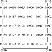
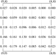
Figure 6: For one hole on 10 by 10 lattice, we plot $Z_{-,k}$ of pBCSwf (left, $\chi=1$, $\Delta=0.55$) and pSDwf (right, $\chi=1$, $\Delta=0.55$, $\frac{\tilde{\beta}_{1}}{\tilde{\beta}_{0}}=-0.3$, $\frac{\tilde{\beta}_{2}}{\tilde{\beta}_{0}}=0.3$, $\frac{\tilde{\beta}_{1}}{\tilde{\beta}_{0}}=-0.1$). pBCSwf has almost constant $Z_{-}$ along diagonal direction from $(\pi,0)$ to $(0,\pi)$; while pSDwf has $Z_{-}$ suppressed at anti-nodal point.

In Fig.7 we compare the energy dispersion of one-hole quasi-particle excitations of pBCSwf and pSDwf. The energy of a doped hole in pSDwf is $0.38t$ lower than that of a hole in pBCSwf.

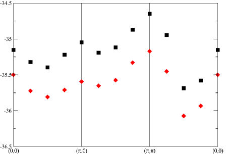
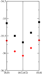
Figure 7: Quasi-particle spectrum for one hole on 10 by 10 lattice. $t=1$, $t^{\prime}=-0.3$, $t^{\prime\prime}=0.2$ and $J=0.3$. The black square shows the spectrum of $d$-wave pBCSwf with $\chi=1$ and $\Delta=0.55$, and the red diamond shows the spectrum of pSDwf with $\chi=1$, $\Delta=0.55$, $\frac{\tilde{\beta}_{1}}{\tilde{\beta}_{0}}=-0.3$, $\frac{\tilde{\beta}_{2}}{\tilde{\beta}_{0}}=0.3$ and $\frac{\tilde{\beta}_{3}}{\tilde{\beta}_{0}}=-0.1$. One can see the first hole doped to $(\pi/2,\pi/2)$. The energy of a doped hole in pSDwf is $0.38t$ lower than that of a hole in pBCSwf.

IV.3 Electron doped case

In electron-doped case, one can do a particle-hole transformation, then multiply a $(-1)$ for the odd lattice electron operators. By doing so, the original electron-doped $t$-$J$ model with parameters $t,t^{\prime},t^{\prime\prime},J$ transformed into hole-doped $t$-$J$ model with parameters $t,-t^{\prime},-t^{\prime\prime},J$, together with a $(\pi,\pi)$ shift in momentum space.

The approach outlined in Eq.(111) and Eq.(112) still applies here. But because of the particle-hole transformation, we are calculating $Z_{+}$ of the original electron-doped system. Because $t^{\prime}>0$ and $t^{\prime\prime}<0$, to favor longer range hoppings, we must have $\tilde{\beta}_{2}<0$ and $\tilde{\beta}_{3}>0$, which differ from hole-doped case by a sign flip. As a result, the $Z_{+}$ now will be suppressed at nodal point, but enhanced at the anti-nodal point. This is exactly what people observed in exact diagonalizationLeung et al. (1997).

We did a variational search for the optimal variational parameters for pBCSwf with longer range hoppings $\chi^{\prime}$ and $\chi^{\prime\prime}$, and pSDwf with non-local mixings. In Table 3 we compare the energy of pBCSwf and pSDwf with 2 electron doped on 10 by 10 lattice. In Fig.8 we plot the $Z_{+}$ map of pSDwf, one can see pSDwf has spectral weight of anti-dichotomy shape.

wavefunction	$\frac{\Delta}{\chi}$	$\frac{\chi^{\prime}}{\chi}$	$\frac{\chi^{\prime\prime}}{\chi}$	$\frac{\tilde{\beta}_{1}}{\tilde{\beta}_{0}}$	$\frac{\tilde{\beta}_{2}}{\tilde{\beta}_{0}}$	$\frac{\tilde{\beta}_{3}}{\tilde{\beta}_{0}}$	$\begin{array}[]{c}\mbox{total energy}\\ \mbox{per bond}\end{array}$	$\begin{array}[]{c}\langle\vec{S}_{i}\cdot\vec{S}_{i+1}\rangle\\ \mbox{per bond}\end{array}$	$T_{1}$	$T_{2}$	$T_{3}$
pBCSwf	0.55	0	0	0	0	0	-0.1884$\pm$0.0001	-0.2977$\pm$0.0002	2.64$\pm$0.01	0.52$\pm$0.01	0.48$\pm$0.01
pBCSwf(optimal)	0.55	0.2	0.0	0	0	0	-0.1888$\pm$0.0001	-0.2964$\pm$0.0002	2.61$\pm$0.01	0.70$\pm$0.02	0.20$\pm$0.02
pSDwf(optimal)	0.55	0	0	-0.5	-0.3	0.3	-0.1910$\pm$0.0001	-0.2971$\pm$0.0002	2.57$\pm$0.01	0.86$\pm$0.02	-0.72$\pm$0.02

Table 3: Two electrons on 10 by 10 lattice. $t=1$, $t^{\prime}=-0.3$, $t^{\prime\prime}=0.2$ and $J=0.3$, and we mapped it into a hole-doped model with $t=1$, $t^{\prime}=0.3$, $t^{\prime\prime}=-0.2$ and $J=0.3$ with a $(\pi,\pi)$ shift in momentum space. $T_{1}$, $T_{2}$ and $T_{3}$ stand for nearest neighbor hopping per hole $\frac{1}{N_{h}}\sum_{i,\delta=\pm\hat{x},\pm\hat{y}}\langle c_{i}^{{\dagger}}c_{i+\delta}\rangle$, next nearest neighbor hopping per hole $\frac{1}{N_{h}}\sum_{i,\delta=\pm(\hat{x}+\hat{y}),\pm(\hat{x}-\hat{y})}\langle c_{i}^{{\dagger}}c_{i+\delta}\rangle$ and third nearest neighbor hopping per hole $\frac{1}{N_{h}}\sum_{i,\delta=\pm 2\hat{x},\pm 2\hat{y}}\langle c_{i}^{{\dagger}}c_{i+\delta}\rangle$ respectively. We compare pBCSwf of $d$-wave ansatz, pBCSwf with longer range hoppings $\chi^{\prime}$ and $\chi^{\prime\prime}$, and pSDwf with non-local mixings. The best trial pSDwf has energy lowered by 1.2% from the best trial pBCSwf with longer range hoppings. And comparing the first line and the last line which have the same spin correlations, we find that the energy of a doped electron in pSDwf is $0.26t$ lower than that of an electron in pBCSwf.

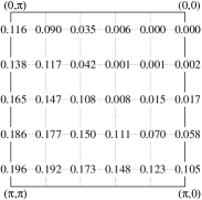
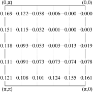
Figure 8: For one electron on 10 by 10 lattice, we plot $Z_{+,k}$ of pBCSwf(left, $\chi=1$, $\Delta=0.55$) and pSDwf(right, $\chi=1$, $\Delta=0.55$, $\frac{\tilde{\beta}_{1}}{\tilde{\beta}_{0}}=-0.5$, $\frac{\tilde{\beta}_{2}}{\tilde{\beta}_{0}}=-0.3$, $\frac{\tilde{\beta}_{1}}{\tilde{\beta}_{0}}=0.3$). By particle-hole symmetry, the $Z_{+}$ of one electron pBCSwf is identical to the $Z_{-}$ of one hole pBCSwf together with a $(\pi,\pi)$ momentum shift. pBCSwf has almost constant $Z_{+}$ along the direction from $(\pi,0)$ to $(0,\pi)$; while pSDwf has $Z_{+}$ suppressed at nodal point and enhanced at anti-nodal point.

In Fig.9 we compare the energy dispersion of one-electron quasi-particle excitations of pBCSwf and pSDwf. The energy of a doped electron in pSDwf is $0.25t$ lower than that of an electron in pBCSwf.

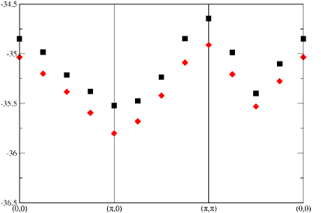
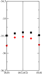
Figure 9: Quasi-particle spectrum for one electron on 10 by 10 lattice. $t=1$, $t^{\prime}=-0.3$, $t^{\prime\prime}=0.2$ and $J=0.3$ (one can map it into a hole-doped model with $t=1$, $t^{\prime}=0.3$, $t^{\prime\prime}=-0.2$ and $J=0.3$ with a $(\pi,\pi)$ shift in momentum space.). The black square shows the spectrum of $d$-wave pBCSwf with $\chi=1$ and $\Delta=0.55$, and the red diamond shows the spectrum of pSDwf with $\chi=1$, $\Delta=0.55$, $\frac{\tilde{\beta}_{1}}{\tilde{\beta}_{0}}=-0.5$, $\frac{\tilde{\beta}_{2}}{\tilde{\beta}_{0}}=-0.3$ and $\frac{\tilde{\beta}_{3}}{\tilde{\beta}_{0}}=0.3$. One can see the first electron doped to $(\pi,0)$. The energy of a doped electron in pSDwf is $0.25t$ lower than that of an electron in pBCSwf.

IV.4 A prediction

In hole-doped and electron-doped case, $t>0$ and $t^{\prime}$ and $t^{\prime\prime}$ have opposite signs, and as a result $Z_{-}$ develops strong $k$ dependence along diagonal direction. What if $t^{\prime}$ and $t^{\prime\prime}$ have the same sign? If both $t^{\prime}>0$ and $t^{\prime\prime}>0$, one expects that $\tilde{\beta}_{2}<0$ and $\tilde{\beta}_{3}<0$ to favor longer range hoppings. But they drive the modulation of $Z_{-}$ in opposite ways. As a result, one expects that for certain ratio of values of $t^{\prime}>0$ and $t^{\prime\prime}>0$ of order 1, their effects cancel and $Z_{-}$ remains constant along the diagonal direction, but with an enhanced value of $Z_{-}$ than the case of pure $t$-$J$ model. Similarly for certain ratio of values of $t^{\prime}<0$ and $t^{\prime\prime}<0$ of order 1, $Z_{-}$ remains constant along the diagonal direction, but with a suppressed value of $Z_{-}$ than the case of pure $t$-$J$ model. These predictions can be checked by exact diagonalization.

IV.5 pBCSwf with longer range hoppings

One can view pSDwf as an improved pBCSwf. We choose the $d$-wave pairing wavefunction $b(k)$ with only nearest hopping $\chi$ and pairing $\Delta$ parameters. Then $\beta_{2}$ and $\beta_{3}$ encode some second-neighbor and third-neighbor correlations. The price to pay is to include more than one Slater determinants in spin basis. One may naturally ask, suppose we insist working on pBCSwf, if one puts in longer range hopping parameters like $\chi^{\prime}$ and $\chi^{\prime\prime}$ in the pairing wavefunction $b(k)$, one also encodes some second-neighbor and third-neighbor correlations, which may lower the second-neighbor and third-neighbor hopping energies. But in this way one can still work with a single Slater determinant. If our pSDwf with no-local mixing is physically similar to pBCSwf with longer range hoppings, why should one bother to work with many Slater determinants?

We want to emphasize that our pSDwf is physically different from pBCSwf even after we include longer range hoppings $\chi^{\prime}$ and $\chi^{\prime\prime}$. We note that, in the infinite-lattice limit with a few holes, the pBCSwf cannot have longer range hoppings (i.e. $\chi^{\prime}=\chi^{\prime\prime}=0$). Otherwise we are considering some other spin wavefunction instead of $d$-wave wavefunction, which will increase the spin energy by a finite amount per site. Therefore $\chi^{\prime}$ and $\chi^{\prime\prime}$ have to vanish in low doping limit. In contrast, for our pSDwf, the the spin energy is not affected by finite $\beta_{i}$ in the zero doping limit. Thus in the low doping limit, the spin energy is perturbed only slightly by a finite $\beta_{2}$ and $\beta_{3}$. On the other hand a finite $\beta_{2}$ and $\beta_{3}$ make the hopping energy much larger than that of pBCSwf. So in the infinite-lattice limit with a few holes, $\beta_{i}$ will be finite and the energy of one hole will be lowered by a finite amount by turning on a finite $\beta_{i}$.

Physically this means that $\beta_{2}$ and $\beta_{3}$ characterize the charge correlations, while $\chi^{\prime}$ and $\chi^{\prime\prime}$ characterize the spin correlations. The above claim is supported by 2-hole system on larger lattice, i.e., by lower the doping. In Table 4 we list the energies of pBCSwf with longer range hopping and pSDwf on 14 by 14 lattice. Comparing with Table 2 one can see the spin energy for pSDwf is lowered further than that for pBCSwf.

wavefunction	$\frac{\Delta}{\chi}$	$\frac{\chi^{\prime}}{\chi}$	$\frac{\chi^{\prime\prime}}{\chi}$	$\frac{\tilde{\beta}_{1}}{\tilde{\beta}_{0}}$	$\frac{\tilde{\beta}_{2}}{\tilde{\beta}_{0}}$	$\frac{\tilde{\beta}_{3}}{\tilde{\beta}_{0}}$	$\begin{array}[]{c}\mbox{total energy}\\ \mbox{per bond}\end{array}$	$\begin{array}[]{c}\langle\vec{S}_{i}\cdot\vec{S}_{i+1}\rangle\\ \mbox{per bond}\end{array}$	$T_{1}$	$T_{2}$	$T_{3}$
pBCSwf	0.55	0	0	0	0	0	-0.1793$\pm$0.0001	-0.3075$\pm$0.0002	2.65$\pm$0.02	0.43$\pm$0.02	0.65$\pm$0.02
pBCSwf	0.55	-0.4	0	0	0	0	-0.1796$\pm$0.0001	-0.3043$\pm$0.0002	2.66$\pm$0.02	0.02$\pm$0.02	1.21$\pm$0.02
pSDwf	0.55	0	0	-0.3	0.3	-0.1	-0.1815$\pm$0.0001	-0.3058$\pm$0.0002	2.86$\pm$0.02	-0.49$\pm$0.02	0.87$\pm$0.02

Table 4: Two holes on 14 by 14 lattice. $t=1$, $t^{\prime}=-0.3$, $t^{\prime\prime}=0.2$ and $J=0.3$. $T_{1}$, $T_{2}$ and $T_{3}$ stand for nearest neighbor hopping, next nearest neighbor hopping and third nearest neighbor hopping respectively. Although the spin energy of pBCSwf with finite longer range hoppings $\chi^{\prime}=-0.4$ is slightly lower than that of pSDwf on 10 by 10 lattice, it is much higher on 14 by 14 lattice.

Another way to see that these two wavefunctions are different is by calculating $Z_{-}$. Numerical results show that pSDwf has dichotomy whereas pBCSwf does not. Actually on the mean-field level, a negative $\chi^{\prime}$ and/or positive $\chi^{\prime\prime}$ even make the $Z_{-}$ larger on the anti-nodal point than on the nodal point. After projection, we observe that $Z_{-}$ still remains almost constant along the diagonal direction for pBCSwf with longer range hoppings. In Fig.10 we plot the $Z_{-}$ map of pBCSwf with longer range hopping $\chi^{\prime}=-0.4$.

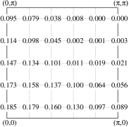
Figure 10: For one hole on 10 by 10 lattice, we plot $Z_{-,k}$ of pBCSwf with longer range hopping $\chi^{\prime}=-0.4$ ($\chi=1$, $\Delta=0.55$).

V Conclusion

In this paper we studied a new type of variational wavefunction, pSDwf. It can be viewed as an improved pBCSwf, and the improvement is that pSDwf correctly characterizes the charge dynamics and the correlation between the doped holes/electrons and the nearby spins. This physics was missed by the previous pBCSwf. As a result, pSDwf correctly reproduces the dichotomy of hole-doped and electron-doped Mott insulator.

In pSDwf, we introduced two types of fermions, spinon $f$ and dopon $d$. Spinons $f$ carry spin but no charge. They form a $d$-wave paired state that describes the spin liquid background. Dopons $d$ carry both spin and charge and correspond to a bare doped hole. The mixing between spinons and dopons described by $\beta_{0}$, $\beta_{1}$, $\beta_{2}$ and $\beta_{3}$ leads to a $d$-wave superconducting state. The charge dynamics (such as electron spectral function) is determined by those mixings. $\beta_{0}$ is the on-site mixing (or local mixing), and $\beta_{1}$, $\beta_{2}$ and $\beta_{3}$ are non-local mixings corresponding to mixing with first, second and third neighbors respectively. If pSDwf has only local mixing, it is identical to pBCSwf. With non-local mixings, pSDwf corresponds to pBCSwf with hopping terms acting on it. Therefore the wavefunction develops finite non-local mixings to lower the hopping energies. In particular, for the hole-doped case, to lower $t^{\prime}$ and $t^{\prime\prime}$ energies, the mixing is described by $\beta_{2}>0$ and $\beta_{3}<0$.

The pSDwf can also be obtained by projecting the spinon-dopon mean-field wavefunction into the physical subspace. Therefore, one expects that some properties of pSDwf can be understood from the mean-field theory. In the mean-field theory, it is clear that the modulation of $Z_{-,k}$ in $k$ space is controlled by the non-local mixings. Our numerical calculation of $Z_{-,k}$ shows that the above mean-field result is valid even for the projected wave function. We find that $\beta_{2}>0$ and $\beta_{3}<0$ give exactly the dichotomy of $Z_{-,k}$ observed in the hole doped samples. Because $\beta_{2}>0$ and $\beta_{3}<0$ are driven by $t^{\prime}$ and $t^{\prime\prime}$, the dichotomy is also driven by $t^{\prime}$ and $t^{\prime\prime}$. Thus to lower the hopping energy, the spectral weight is suppressed in some region in $k$-space. This result conflicts a naive guess: to lower the hopping energy, the excitation should be more quasi-particle like. We also predict that the dichotomy will go away if $t^{\prime}$ and $t^{\prime\prime}$ have the same sign and similar magnitude. In summary, we found a mean-field theory and the associated trial wavefunction capturing the dichotomy physics.

Traditionally, in projected wavefunction variational approach, for example pBCSwf, people use wavefunctions which in real space correspond to a single Slater determinant. The reason to do so is simply to make the computation easier. Our study shows what kinds of important physics that may be missed by doing so. In real space, the pSDwf is sum of $(1+n_{shift})^{n_{hole}}$ number of Slater determinants, because each hole can either do not hop, or hop into one of $n_{shift}$ sites. So our calculation is limited to few-hole cases. However, the idea of introducing many Slater determinant is quite general. For example, one can study another improved pBCSwf, which allows each hole to hop once but forbids two holes hopping together, therefore the number of Slater determinant is $(1+n_{shift})n_{hole}$ and many-hole cases are computationally achievable. This new improved pBCSwf is the first order approximation of pSDwf and remains to be studied. For a long time there is a puzzle that doped Mott-insulator (ie the spin disordered metallic state) seems to be energetically favorable only at high doping $x>0.3$. For $x<0.3$ the doped spin density wave state have a lower energy. Our pSDwf may push this limit down to low doping which agrees with experiments better. This is because that including many Slater determinants can lower the energy per hole by a significant amount (about $0.4t$).

As we have stressed, pSDwf provides a better description of spin-charge correlation, or more precisely, the spin configuration near a doped hole. This allows us to reproduce the dichotomy in quasiparticle spectral weights observed in experiments. The next question is whether the better understanding of the spin-charge correlation can lead to new experimental predictions. In the following, we will describe one such prediction in quasi-particle current distribution.

We know that a finite supercurrent $\bm{J}_{s}$ shifts the superconducting quasiparticle dispersion $E_{\bm{k}}$. To the linear order in $\bm{J}_{s}$, we have

$$E_{\bm{k}}(\bm{A})=E_{\bm{k}}(0)+c^{-1}\bm{j}_{\bm{k}}\cdot\bm{A},$$

where $c$ is the speed of light and we have introduced the vector potential $\bm{A}$ to represent the supercurrent: $\bm{J}_{s}=\frac{n_{s}e^{2}}{mc}\bm{A}$. $\bm{j}_{\bm{k}}$ is a very important function that characterizes how excited quasiparticles affect superfluid density $\rho_{S}$. We call $\bm{j}_{\bm{k}}$ quasiparticle current. According to the BCS theory

$$\bm{j}_{\bm{k}}=e\frac{\partial\epsilon_{\bm{k}}}{\partial\bm{k}}=e\bm{v}_{\text{normal}},$$ (116)

where $\epsilon_{\bm{k}}$ is the normal state dispersion which is roughly given by $\epsilon_{\bm{k}}=-2t[\cos(k_{x})+\cos(k_{y})]$.

The previous studyNave et al. (2006) of quasi-particle current for pBCSwf shows that the quasi-particle current is roughly given by the BCS result (116) scaled down by a factor $\alpha$. Such a quasi-particle current has a smooth distribution in $k$-space. Here we would like to stress that since the charge dynamics is not capture well by the pBCSwf, the above result from pBCSwf may not be reliable. We expect that the quasi-particle current of pSDwf should has a strong $k$-dependence, ie a large quasi-particle current near the nodal point where $Z_{k}$ is large and small quasi-particle current near the anti-nodal point where $Z_{k}$ is small. Such a quasi-particle current distribution may explain the temperature dependence of superfluid density Liang et al. (2005).

Indeed, the mean-field spinon-dopon approach does give rise to a very different quasi-particle current distribution which roughly follows $Z_{k}$. For more detailed study in this direction and possible experimental tests, see Ref. Ribeiro et al. (to be published).

We would like to thank Cody Nave, Sung-Sik Lee, P. A. Lee for helpful discussions. This work was supported by NSF grant No. DMR-0433632

Appendix A A simple algorithm to do local projection

Suppose the wavefunction before projection is the ground state of some fermionic quadratic Hamiltonian. One can always diagonalize the Hamiltonian so that all two-point correlation functions of fermion operators can be calculated exactly. For our SDwf, that means quantities like $\langle f_{i}^{{\dagger}}f_{j}\rangle$, $\langle d_{i}^{{\dagger}}f_{j}\rangle$,$\langle d_{i}^{{\dagger}}d_{j}\rangle$… can be calculated.

Projection is supposed to remove the unphysical states. For a site $i$, the following operator removes the unphysical states.

$$P_{i}= n_{f,i}(n_{f,i}-2)(\frac{1}{2}n_{d,i}^{2}-\frac{1}{2}n_{d,i}+1)$$

$$\cdot(1-\frac{1}{2}n_{d,i}(\vec{S}_{f,i}+\vec{S}_{d,i})^{2}).$$ (117)

It obviously ensures that $n_{f,i}=1$, $n_{d,i}\neq 2$ and $f$ and $d$ fermions form local singlet. To calculate energy, we do local projection on the relevant sites. For example, to calculate the $J$ term energy, one actually calculates

$$\langle\vec{S}_{i}\cdot\vec{S}_{j}\rangle_{prj}=\frac{\langle P_{i}P_{j}(\vec{S}_{f,i}+\vec{S}_{d,i})\cdot(\vec{S}_{f,j}+\vec{S}_{d,j})P_{i}P_{j}\rangle}{\langle P_{i}P_{j}\rangle}.$$ (118)

The denominator accounts for the wavefunction normalization due to projection. One can write operators $P_{i}\vec{S}_{i}\cdot\vec{S}_{j}P_{j}$ and $P_{i}\vec{S}_{i}\cdot\vec{S}_{j}P_{j}$ in terms of fermion operators. By Wick’s theorem, the expectation values of these operators reduce to a sum of products of fermion two-point correlation functions, which are known. Similarly for $t$ term energy, one calculates for example,

$$\langle c_{i\uparrow}^{{\dagger}}c_{j\uparrow}\rangle_{prj}=\frac{\langle P_{i}P_{j}f_{i\uparrow}^{{\dagger}}h_{j}^{{\dagger}}h_{i}f_{j\uparrow}P_{i}P_{j}\rangle}{\langle P_{i}P_{j}\rangle},$$ (119)

where $h_{i}^{{\dagger}}=\frac{1}{\sqrt{2}}(f_{i\uparrow}^{{\dagger}}d_{i\downarrow}^{{\dagger}}-f_{i\downarrow}^{{\dagger}}d_{i\uparrow}^{{\dagger}})$ is the operator that creates a hole at site $i$.

One may ask whether we can do local projections on more and more sites, then the result will be closer and closer to the one of full projection. Unfortunately this cannot be done, because the number of terms in the summation when we expand $P_{i1}P_{i2}\ldots P_{in}$ increases exponentially fast as we increase $n$. Therefore we are limited to few sites. The above method can only be viewed as some renormalized mean-field approach.

References

- Damascelli et al. (2003) A. Damascelli, Z. Hussain, and Z.-X. Shen, Rev. Mod. Phys. 75, 473 (2003).
- Shen and Schrieffer (1997) Z.-X. Shen and J. Schrieffer, Phys. Rev. Lett. 78, 1771 (1997).
- Zhou et al. (2004) X. Zhou, T. Yoshida, D.-H. Lee, W. Yang, V. Brouet, F. Zhou, W. Ti, J. Xiong, Z. Zhao, T. Sasagawa, et al., Phys. Rev. Lett. 92, 187001 (2004).
- Pan et al. (2001) S. Pan, J. O’Neal, R. Badzey, C. Chamon, H. Ding, J. Engelbrecht, Z. Wang, H. Eisaki, S. Uichada, A. Gupta, et al., Nature 413, 282 (2001).
- Howald et al. (2001) C. Howald, P. Fournier, and A. Kapitulnik, Phys. Rev. B 64, 100504 (2001).
- McElroy et al. (2005) K. McElroy, D.-H. Lee, J. E. Hoffman, K. M. Lang, J. Lee, E. W. Hudson, H. Eisaki, S. Uchida, and J. C. Davis, Phys. Rev. Lett. 94, 197005 (2005).
- Leung and Gooding (1995) P. W. Leung and R. J. Gooding, Phys. Rev. B 52, R15711 (1995).
- Leung et al. (1997) P. W. Leung, B. O. Wells, and R. J. Gooding, Phys. Rev. B 56, 6320 (1997).
- Fong et al. (1999) H. Fong, P. Bourges, Y. Sidis, L. Regnault, A. Ivanov, G. Gu, N. Koshizuka, and B. Keimer, Nature 398, 588 (1999).
- Tranquada et al. (1995) J. Tranquada, B. Sternlieb, J. Axe, Y. Nakamura, and S. Uchida, Nature 375, 561 (1995).
- Aeppli et al. (1997) G. Aeppli, T. Mason, S. Hayden, H. Mook, and J. Kulda, Science 278, 1432 (1997).
- Yamada et al. (1998) K. Yamada, C. H. Lee, K. Kurahashi, J. Wada, S. Wakimoto, S. Ueki, H. Kimura, Y. Endoh, S. Hosoya, G. Shirane, et al., Phys. Rev. B 57, 6165 (1998).
- Zhang and Rice (1988) F. Zhang and T. Rice, Phys. Rev. B 37, 3759 (1988).
- Baskaran et al. (1987) G. Baskaran, Z. Zou, and P. Anderson, Solid State Commun. 63, 973 (1987).
- Kotliar and Liu (1988) G. Kotliar and J. Liu, Phys. Rev.B 38, 5142 (1988).
- Lee et al. (2006) P. Lee, N. Nagaosa, and X.-G. Wen, Rev. Mod. Phys. 78, 17 (2006).
- Gros (1988) C. Gros, Phys. Rev. B) 38, 931 (1988).
- Nave et al. (2006) C. Nave, D. Ivanov, and P. Lee, Phys. Rev. B 73, 104502 (2006).
- Bieri and Ivanov (2006) S. Bieri and D. Ivanov, condmat/0608047 (2006).
- Ribeiro and Wen (2005) T. C. Ribeiro and X.-G. Wen, Phys. Rev. Lett. 95, 1 (2005).
- Liang et al. (2005) R. Liang, D. A. Bonn, W. N. Hardy, and D. Broun, Phys. Rev. Lett. 94, 117001 (2005).
- Lee and Nagaosa (1992) P. Lee and N. Nagaosa, Physical Review B 46, 5621 (1992).
- Ribeiro and Wen (2006a) T. C. Ribeiro and X.-G. Wen, Phys. Rev. B 74, 155113 (2006a).
- Ribeiro and Wen (2006b) T. C. Ribeiro and X.-G. Wen, Phys. Rev. Lett. 97, 057003 (2006b).
- Paramekanti et al. (2001) A. Paramekanti, M. Randeria, and N. Trivedi, Phys. Rev. Lett. 87, 217002 (2001).
- Ivanov and Lee (2003) D. A. Ivanov and P. A. Lee, Phys. Rev. B 68, 132501 (2003).
- Ribeiro et al. (to be published) T. C. Ribeiro, X.-G. Wen, and A. Vishwanath (to be published).