Monomer-dimer model in two-dimensional rectangular lattices with fixed dimer density

Abstract

The classical monomer-dimer model in two-dimensional lattices has been shown to belong to the “#P-complete” class, which indicates the problem is computationally “intractable”. We use exact computational method to investigate the number of ways to arrange dimers on $m\times n$ two-dimensional rectangular lattice strips with fixed dimer density $\rho$. For any dimer density $0<\rho<1$, we find a logarithmic correction term in the finite-size correction of the free energy per lattice site. The coefficient of the logarithmic correction term is exactly $-1/2$. This logarithmic correction term is explained by the newly developed asymptotic theory of Pemantle and Wilson. The sequence of the free energy of lattice strips with cylinder boundary condition converges so fast that very accurate free energy $f_{2}(\rho)$ for large lattices can be obtained. For example, for a half-filled lattice, $f_{2}(1/2)=0.633195588930$, while $f_{2}(1/4)=0.4413453753046$ and $f_{2}(3/4)=0.64039026$. For $\rho<0.65$, $f_{2}(\rho)$ is accurate at least to 10 decimal digits. The function $f_{2}(\rho)$ reaches the maximum value $f_{2}(\rho^{*})=0.662798972834$ at $\rho^{*}=0.6381231$, with $11$ correct digits. This is also the monomer-dimer constant for two-dimensional rectangular lattices. The asymptotic expressions of free energy near close packing are investigated for finite and infinite lattice widths. For lattices with finite width, dependence on the parity of the lattice width is found. For infinite lattices, the data support the functional form obtained previously through series expansions.

I Introduction

The monomer-dimer problem has received much attention not only from statistical physics but also from theoretical computer science. As one of the classical lattice statistical mechanics models, the monomer-dimer model was first used to describe the absorption of a binary mixture of molecules of unequal sizes on crystal surface Fowler and Rushbrooke (1937). In the model, the regular lattice sites are either covered by monomers or dimers. The diatomic molecules are modeled as rigid dimers which occupy two adjacent sites in a regular lattice and no lattice site is covered by more than one dimer. The lattice sites that are not covered by the dimers are regarded as occupied by monomers. A central problem of the model is to enumerate the dimer configurations on the lattice. In 1961 an elegant analytical solution was found for a special case of the problem, namely when the planar lattice is completely covered by dimers (the close-packed dimer problem, or dimer-covering problem) Kasteleyn (1961); Temperley and Fisher (1961). For the general monomer-dimer problem where there are vacancies (monomers) in the lattice, there is no exact solution. For three-dimensional lattices, there is even no exact solution for the special case of close-packed dimer problem. One recent advance is an analytic solution to the special case of the problem in two-dimensional lattices where there is a single vacancy at certain specific sites on the boundary of the lattice Tzeng and Wu (2003); Wu (2006a). The monomer-dimer problem also serves as a prototypical problem in the field of computational complexity Garey and Johnson (1979). It has been shown that two-dimensional monomer-dimer problem belongs to the “#P-complete” class and hence is computationally intractable Jerrum (1987).

Even though there is a lack of progress in the analytical solution to the monomer-dimer problem, many rigorous results exist, such as series expansions Nagle (1966); Gaunt (1969); Samuel (1980), lower and upper bounds on free energy Bondy and Welsh (1966); Friedland and Peled (2005), monomer-monomer correlation function of two monomers in a lattice otherwise packed with dimers Fisher and Stephenson (1963), locations of zeros of partition functions, Heilmann and Lieb (1972); Gruber and Kunz (1971), and finite-size correction Ferdinand (1967). Some approximate methods have also been proposed Chang (1939); Baxter (1968); Nemirovsky and Coutinho-Filho (1989); Lin and Lai (1994). The monomer-dimer constant $h_{d}$ (the exponential growth rate) of the number of all configurations with different number of dimers has also been calculated Baxter (1968); Friedland and Peled (2005). By using sequential importance sampling Monte Carlo method, the dimer covering constant for a three-dimensional cubic lattice has been estimated Beichl and Sullivan (1999). The importance of monomer-dimer model also comes from the fact that there is one to one mapping between the Ising model and the monomer-dimer model: the Ising model in the absence of an external field is mapped to the pure dimer model Kasteleyn (1963); Fisher (1966); Fan and Wu (1970); McCoy and Wu (1973), and the Ising model in the presence of an external field is mapped to the general monomer-dimer model Heilmann and Lieb (1972).

The major purposes of this paper are (1) to show it is possible to calculate accurately the free energy of the monomer-dimer problem in two-dimensional rectangular lattices at a fixed dimer density by using the proposed computational methods (Sections II, IV, VI, and VII), and (2) to use the computational methods to probe the physical properties of the monomer-dimer model, especially at the high dimer density limit (Section VIII). The high dimer density limit is considered to be more difficult and more interesting than the low dimer density limit. The major result is the asymptotic expression Eq. 24. The third purpose of the paper is to introduce the asymptotic theory of Pemantle and Wilson Pemantle and Wilson (2002), which not only gives a theoretical explanation of the origin of the logarithmic correction term found by computational methods reported in this paper (Section III), but also has the potential to be applicable to other statistical models.

The following notation and definitions will be used throughout the paper. The configurational grand canonical partition function of the monomer-dimer system in a $m\times n$ two-dimensional lattice is

$$Z_{m,n}(x)=a_{N}(m,n)x^{N}+a_{N-1}(m,n)x^{N-1}+\cdots+a_{0}(m,n)$$ (1)

where $a_{s}(m,n)$ is the number of distinct ways to arrange $s$ dimers on the $m\times n$ lattice, $N=\lfloor mn/2\rfloor$, and $x$ can be taken as the activity of a dimer. The average number of sites covered by dimers (twice the average number of dimers) of this grand canonical ensemble is given by

$$\theta_{m,n}(x)=\frac{2}{mn}\frac{\partial\ln Z_{m,n}(x)}{\partial\ln x}=\frac{2}{mn}\frac{\sum_{s=1}^{N}a_{s}(m,n)sx^{s}}{\sum_{s=0}^{N}a_{s}(m,n)x^{s}}.$$ (2)

The limit of this average for large lattices is denoted as $\theta(x)$: $\theta(x)=\lim_{m,n\rightarrow\infty}\theta_{m,n}(x)$. In general we use $\theta_{d}(x)$ for the average number of sites covered by dimers in a $d$-dimensional infinite lattice when the dimer activity is $x$.

The total number of configurations of dimers is given by $Z_{m,n}(1)$ at $x=1$, and the monomer-dimer constant for a two-dimensional infinite lattice is defined as

$$h_{2}=\lim_{m,n\rightarrow\infty}\frac{\ln Z_{m,n}(1)}{mn}.$$ (3)

In general, we denote $h_{d}$ as the monomer-dimer constant for a $d$-dimensional infinite lattice, and $h_{d}(x)$ as the grand potential per lattice site at any dimer activity $x$. For a two-dimensional infinite lattice,

$$h_{2}(x)=\lim_{m,n\rightarrow\infty}\frac{\ln Z_{m,n}(x)}{mn}.$$ (4)

In this paper we focus on the number of dimer configurations at a given dimer density $\rho$. In this sense we are working on the canonical ensemble. The connection between the canonical ensemble and the grand canonical ensemble is discussed in Appendix A. We define the dimer density for the canonical ensemble as the ratio

$$\rho=\frac{2s}{mn}.$$ (5)

When the lattice is fully covered by dimers, $\rho=1$. For a $m\times n$ lattice, the number of dimers at a given dimer density is $s=\frac{mn\rho}{2}$. In the following we use $a_{m,n}(\rho)$ as the number of distinct dimer and monomer configurations at the given dimer density $\rho$. By using this definition, Eq. 1 can be rewritten as

$$Z_{m,n}(x)=\sum_{0\leq\rho\leq 1}a_{m,n}(\rho)x^{mn\rho/2}.$$ (6)

The free energy per lattice site at a given dimer density $\rho$ is defined as

$$f_{m,n}(\rho)=\frac{\ln a_{m,n}(\rho)}{mn}$$

and the free energy at a given dimer density for a semi-infinite lattice strip $\infty\times n$ is

$$f_{\infty,n}(\rho)=\lim_{m\rightarrow\infty}\frac{\ln a_{m,n}(\rho)}{mn}=\lim_{m\rightarrow\infty}f_{m,n}(\rho).$$

For infinite lattices where both $m$ and $n$ go to infinity, the free energy is

$$f_{2}(\rho)=f_{\infty,\infty}(\rho)=\lim_{m,n\rightarrow\infty}\frac{\ln a_{m,n}(\rho)}{mn}=\lim_{n\rightarrow\infty}f_{\infty,n}(\rho).$$

We use the subscript $d$ in $f_{d}(\rho)$ to indicate the dimension of the infinitely large lattice. From the exact result Kasteleyn (1961); Temperley and Fisher (1961) we know $f_{2}(\rho)$ at $\rho=1$

$$f_{2}(1)=\frac{G}{\pi}=0.291560904$$

where $G$ is the Catalan’s constant. For other values of $\rho>0$, no analytical result is known, although several bounds are developed Bondy and Welsh (1966); Friedland and Peled (2005). We will show below that by using the exact calculation method developed previously Kong (1999, 2006a, 2006b), we can calculate $f_{2}(\rho)$ at an arbitrary dimer density $\rho$ with high accuracy.

The article is organized as follows. In Section II, the computational method is outlined. In Section III, we show a logarithmic correction term in the finite-size correction of $f_{m,n}(\rho)$ for any fixed dimer density $0<\rho<1$. The coefficient of this logarithmic correction term is exactly $-1/2$, for both cylinder lattices and lattices with free boundaries. We give a theoretical explanation for this logarithmic correction term and its coefficient using the newly developed asymptotic theory of Pemantle and Wilson Pemantle and Wilson (2002). In this section we point out the universality of this logarithmic correction term with coefficient of $-1/2$. This term is not unique to the monomer-dimer model: a large class of lattice models has this term when the “density” of the models is fixed. More discussions of applications of this asymptotic method to the monomer-dimer model in particular, and statistical models in general, can be found in Section IX. In Section IV we calculate $f_{\infty,n}(\rho)$ on lattice strips $\infty\times n$ for $n=1,\dots,17$ with cylinder boundary condition. The sequence of $f_{\infty,n}(\rho)$ on cylinder lattices converges very fast so that we can obtain $f_{2}(\rho)$ quite accurately. To the best of our knowledge, the results presented here are the most accurate for monomer-dimer problem in two-dimensional rectangular lattices at an arbitrary dimer density. In Section V similar calculations of $f_{\infty,n}(\rho)$ are carried out on lattice strips $\infty\times n$ with free boundaries for $n=1,\dots,16$. Compared with the sequence with cylinder boundary condition, the sequence $f_{\infty,n}(\rho)$ with free boundaries converges slower. In Section VI, the position and values of the maximum of $f_{2}(\rho)$ are located: $f_{2}(\rho^{*})=0.662798972834$ at $\rho^{*}=0.6381231$. These results give an estimation of the monomer-dimer constant with $11$ correct digits. The previous best result is with $9$ correct digits Friedland and Peled (2005). The results are also compared with those obtained by series expansions and field theoretical methods. The maximum value of $f_{2}(\rho)$ is equal to the two-dimensional monomer-dimer constant $h_{2}$. This is one special case of the more general relations between the calculated values in the canonical ensemble and those in the grand canonical ensemble, and these relations are further discussed in Appendix A. In Section VII, the relations developed in Appendix A are used to compare the results of the computational method presented in this paper with those of Baxter Baxter (1968). For monomer-dimer model, the more interesting properties are at the more difficult high dimer density limit. In Section VIII asymptotic behavior of the free energy $f_{\infty,n}(\rho)$ is examined for high dimer density near close packing. For lattices with finite width, a dependence of the free energy $f_{\infty,n}(\rho)$ on the parity of the lattice width $n$ is found (Eq. 22), consistent with the previous results when the number of monomers is fixed Kong (2006b). The combination of the results in this section and those of Section III leads to the asymptotic expression Eq. 24 for near close packing dimer density. The asymptotic expression of $f_{2}(\rho)$, the free energy on an infinite lattice, is also investigated near close packing. The results support the functional forms obtained previously through series expansions Gaunt (1969), but quantitatively the value of the exponent is lower than previously conjectured. In Appendix B we put together in one place various explicit formulas for the one-dimensional lattices ($n=1$). These formulas can be used to check the formulas developed for the more general situations where $n>1$. As an illustration, an explicit application of the Pemantle and Wilson asymptotic method is also given for $n=1$.

II Computational methods

The basic computational strategy is to use exact calculations to obtain a series of partition functions $Z_{m,n}(x)$ of lattice strips $m\times n$. Then for a given dimer density $\rho$, $f_{m,n}(\rho)$ can be calculated using arbitrary precision arithmetic. By fitting $f_{m,n}(\rho)$ to a given function (Sections IV, V, and VIII), $f_{\infty,n}(\rho)$ can be estimated with high accuracy. From $f_{\infty,n}(\rho)$, $f_{2}(\rho)$ can then be estimated using the special convergent properties of the sequence $f_{\infty,n}(\rho)$ on the cylinder lattice strips (Section IV).

II.1 Calculation of the partition functions

The computational methods used here have been described in details previously Kong (1999, 2006a, 2006b). The full partition functions (Eq. 1) are calculated recursively for lattice strips on cylinder lattices and lattices with free boundaries. As before, all calculations of the terms $a_{s}(m,n)$ in the partition functions use exact integers, and when logarithm is taken to calculate free energy $f_{m,n}(\rho)$, the calculations are done with precisions much higher than the machine floating-point precision. The bignum library used is GNU MP library (GMP) for arbitrary precision arithmetic (version 4.2) Granlund (2006). The details of the calculations on lattices with free boundaries can be found in Ref. Kong, 2006a, so in the following only information on cylinder lattices is given.

For a $m\times n$ lattice strip, a square matrix $M_{n}$ is set up based on two rows of the lattice strip with proper boundary conditions. The vector $\Omega_{m}$, which consists of partition function of Eq. 1 as well as other contracted partition functions Kong (1999), is calculated by the following recurrence

$$\Omega_{m}=M_{n}\Omega_{m-1}.$$ (7)

Similar recursive method has also been used for other combinatorial problems, such as calculation of the number of independent sets Calkin and Wilf (1998). For a cylinder lattice strip, the matrix $M_{n}$ is constructed in a similar way as that with free boundaries Kong (2006a). The total valid number ($v_{c}(n)$) and unique number ($u_{c}(n)$) of configurations are given respectively by the generating function $\sum_{n}v_{c}(n)x^{n}=x(3+x-x^{3})/(1-3x-x^{2})/(x-1)/(x+1)$ and the formula

$$u_{c}(n)=\sum_{d\backslash n}\frac{\varphi(d)2^{n/d}}{2n}+\begin{cases}2^{(n-1)/2}&\text{if $n$ odd}\\ 2^{n/2-1}+2^{n/2-2}&\text{if $n$ even}\end{cases}$$

where $\varphi(m)$ is Euler’s totient function, which gives the number of integers relatively prime to integer $m$. The size of matrix $M_{n}$ is $u_{c}(n)\times u_{c}(n)$. The first $17$ terms of the sequence $v_{c}(n)$ are: $3$, $10$, $36$, $118$, $393$, $1297$, $4287$, $14158$, $46764$, $154450$, $510117$, $1684801$, $5564523$, $18378370$, $60699636$, $200477278$, and $662131473$. The first $17$ terms of the sequence $u_{c}(n)$ are: $2$, $3$, $4$, $6$, $8$, $13$, $18$, $30$, $46$, $78$, $126$, $224$, $380$, $687$, $1224$, $2250$, and $4112$. It is noted that the sequence $u_{c}(n)$ is exactly the same as that shown in column 2, Table 1 of Ref. Friedland and Peled, 2005. Calculations based on the dominant eigenvalues of the matrices of the cylinder lattice strips for $n=4$, $6$, $8$, and $10$ are carried out by Runnels Runnels (1970). The sizes of $M_{n}$ for cylinder lattice strips are smaller when compared with the corresponding numbers for lattice strips with free boundaries Kong (2006a), which allows for calculations on wider lattice strips. For cylinder lattice strips, full partition functions are calculated for $n=1,\dots,17$, with length up to $m=1000$ for $n=1,\dots,13$, $m=880$ for $n=14$, $m=669$ for $n=15$, $m=474$ for $n=16$, and $m=325$ for $n=17$. The corresponding numbers for lattice strips with free boundaries are reported in Ref. Kong, 2006a.

II.2 Interpolation for arbitrary dimer density $\rho$

In this paper the main quantity to be calculated is $f_{2}(\rho)$. The starting point of the calculations is the full partition function Eq. 1 for different values of $n$ and $m$. Finite values of $n$ and $m$ only lead to discrete values of dimer density $\rho$, as defined in Eq. 5. For example, when $n=7$ and $m=11$, the number of dimers $s$ takes the values of $0,1,\dots,38$, and dimer density $\rho$ of this lattice can only be one of the following values: $0,2/77,\dots,76/77$. In general, for fixed finite $m$ and $n$, $\rho$ can only be a rational number:

$$\rho=\frac{p}{q}$$

where $p$ and $q$ are positive integers. When $\rho$ is expressed as a rational number, the number of dimers is given by

$$s=\frac{mn\rho}{2}=\frac{mnp}{2q}.$$ (8)

This expression is only meaningful if $mnp$ can be divided by $2q$. When we write the grand canonical partition function in the form of Eq. 6 for finite $m$ and $n$, we implicitly imply that Eq. 8 is satisfied.

In the following we use the rational dimer density $\rho=p/q$ whenever possible so that the value of $a_{m,n}(\rho)$ can be read directly from the partition function of $m\times n$ lattices. Depending on the values of $p$ and $q$, some dimer densities, such as $\rho=1/2$, can be realized in many lattices, while others can only be realized in small number of lattices with special combinations of values of $m$ and $n$. In many situations it becomes impossible to use rational $\rho$. For example, in Section VI the location of the maximum of $f_{2}(\rho)$ is searched within a very small region of $\rho$, and in Section VII, in order to compare the results from different methods, $\rho$ takes the output values of other computational methods Baxter (1968). In such situations, if the rational form of $\rho$ were used, $p$ and $q$ would become so big that not enough data points which satisfy Eq. 8 could be found for the fitting in the $m\times n$ lattice strip. To calculate $f_{m,n}(\rho)$ for an arbitrary real number $\rho$ ($0<\rho<1$), interpolation of the exact data points is needed. Since full partition functions have been calculated for fairly long lattice strips, proper interpolation procedure can yield highly accurate values of $f_{m,n}(\rho)$ for an arbitrary real number $\rho$. For interpolation, we use the standard Bulirsch-Stoer rational function interpolation method Stoer and Bulirsch (1992); Press et al. (1992). For any real number $\rho$, Eq. 8 is used to calculate the corresponding number of dimers $s$, which may not be an integer. On each side of this value of $s$, $30$ exact values of $a_{s}(m,n)$ are used (if possible) in the interpolation. If on one side there are not enough exact data points of $a_{s}(m,n)$, extra data points on the other side of $s$ are used to make the total number of exact data points as $60$. For the high dimer density case (Section VIII), the total number of data points used is changed to $30$. We also take care that no extrapolation is used: if $\rho$ is greater than the maximum dimer density for a given $m\times n$ lattice, the data point from this lattice is not used. Let’s look at the above example of $11\times 7$ lattice again. For this lattice, the highest dimer density is $76/77$. If calculation is done for a dimer density $\rho=0.99$, since $\rho=0.99$ is greater than $76/77\approx 0.987$, the data point from this lattice will not be used in the following steps to avoid inaccuracy introduced by unreliable extrapolations.

II.3 Fitting procedure

The fitting experiments are carried out by using the “fit” function of software gnuplot (version 4.0) Williams and Kelley (2004) on a 64-bit Linux system. The fit algorithm implemented is the nonlinear least-squares (NLLS) Levenberg-Marquardt method Marquart (1963). All fitting experiments use the default value $1$ as the initial value for each parameter, and each fitting experiment is done independently. As done previously Kong (2006a, b), only those $a_{m,n}(\rho)$ with $m\geq 100$ are used in the fitting. Since $a_{m,n}(\rho)$ is calculated for relatively long lattice strips (in the $m$ direction, see Section II.1), the estimates of $f_{\infty,n}(\rho)$ are usually quite accurate, up to $12$ or $13$ decimal place. The accuracy for this fitting step is limited by the machine floating-point precision, since gnuplot uses machine floating-point representations, instead of arbitrary precision arithmetic. We would have used the GMP library to implement a fitting program with arbitrary precision arithmetic. This would increase the accuracy in the estimation of $f_{2}(\rho)$ when $\rho$ is small. For the major objective of this paper, i.e., to investigate the behavior of $f_{2}(\rho)$ when $\rho\rightarrow 1$ (Section VIII), however, the current accuracy is adequate. At high dimer density limit, the convergence of $f_{\infty,n}(\rho)$ towards $f_{2}(\rho)$ is much slower than at low dimer density limit. With lattice width $n\leq 17$ used for the current calculations, $f_{\infty,n}(\rho)$ is far from converging to the machine floating-point precision when $\rho\rightarrow 1$.

III Logarithmic corrections of the free energy at fixed dimer density

For lattice strips $m\times n$ with a fixed width $n$ and a given dimer density $\rho$, the coefficients $a_{m,n}(\rho)$ of the partition functions are extracted to fit the following function:

$$f_{m,n}(\rho)=\frac{\ln a_{m,n}(\rho)}{mn}=c_{0}+\frac{c_{1}}{m}+\frac{c_{2}}{m^{2}}+\frac{c_{3}}{m^{3}}+\frac{c_{4}}{m^{4}}+\frac{\ell}{n}\frac{\ln(m+1)}{m}$$ (9)

where $c_{0}=f_{\infty,n}(\rho)$.

For both cylinder lattices and lattices with free boundaries, the fitting experiments clearly show that $\ell=-1/2$, accurate up to at least six decimal place, for any dimer density $0<\rho<1$. This result holds for both odd $n$ and even $n$. This is in contrast with the results reported earlier for the situation with a fixed number of monomers (or vacancies), where the logarithmic correction coefficient depends on the number of monomers present and the parity of the width of the lattice strip Kong (2006a, b). We notice that a coefficient $-1/2$ also appears in the logarithmic correction term of the free energy studied in Ref. Tzeng and Wu, 2003, which is a special case of the monomer-dimer problem where there is a single vacancy at certain specific sites on the boundary of the lattice.

For the general monomer-dimer model, to our best knowledge, this logarithmic correction term with coefficient of exactly $-1/2$ has not been reported before in the literature. The recently developed multivariate asymptotic theory by Pemantle and Wilson Pemantle and Wilson (2002), however, gives an explanation of this term and its coefficient. This theory applies to combinatorial problems when the multivariate generating function of the model is known. For univariate generating functions, asymptotic methods are well known and have been used for a long time. The situation is quite different for multivariate generating functions. Until recently, techniques to get asymptotic expressions from multivariate generating functions were “almost entirely missing” (for review, see Ref. Pemantle and Wilson, 2002). The newly developed Pemantle and Wilson method applies to a large class of multivariate generating functions in a systematic way. In general the theory applies to generating functions with multiple variables, and for the bivariate case that we are interested in here, the generating function of two variables takes the form

$$F(x,y)=\frac{G(x,y)}{H(x,y)}=\sum_{s,m=0}^{\infty}a_{sm}x^{s}y^{m}$$ (10)

where $G(x,y)$ and $H(x,y)$ are analytic, and $H(0,0)\neq 0$. In this case, Pemantle and Wilson method gives the asymptotic expression as

$$a_{sm}\sim\frac{G(x_{0},y_{0})}{\sqrt{2\pi}}x_{0}^{-s}y_{0}^{-m}\sqrt{\frac{-y_{0}H_{y}(x_{0},y_{0})}{mQ(x_{0},y_{0})}}$$ (11)

where $(x_{0},y_{0})$ is the positive solution to the two equations

$$H(x,y)=0,\qquad mx\frac{\partial{H}}{\partial{x}}=sy\frac{\partial{H}}{\partial{y}}$$ (12)

and $Q(x,y)$ is defined as

$$-(xH_{x})(yH_{y})^{2}-(yH_{y})(xH_{x})^{2}-[(yH_{y})^{2}(x^{2}H_{xx})+(xH_{x})^{2}(y^{2}H_{yy})-2(xH_{x})(yH_{y})(xyH_{xy})].$$

Here $H_{x}$, $H_{y}$, etc. are partial derivatives $\partial{H}/\partial{x}$, $\partial{H}/\partial{y}$, and so on. One of the advantages of the method over previous ones is that the convergence of Eq. 11 is uniform when $s/m$ and $m/s$ are bounded.

For the monomer-dimer model discussed here, with $n$ as the finite width of the lattice strip, $m$ as the length, and $s$ as the number of dimers, we can construct the bivariate generating function $F(x,y)$ as

$$F(x,y)=\sum_{m=0}^{\infty}\sum_{s=0}^{mn/2}a_{s}(m,n)x^{s}y^{m}=\sum_{m=0}^{\infty}Z_{m,n}(x)y^{m}.$$ (13)

For the monomer-dimer model, as well as a large class of lattice models in statistical physics, the bivariate generating function $F(x,y)$ is always in the form of Eq. (10), with $G(x,y)$ and $H(x,y)$ as polynomials in $x$ and $y$. In fact, we can get $H(x,y)$ directly from matrix $M_{n}$ in Eq. (7). It is closely related to the characteristic function of $M_{n}$ Kong (1999): $H(x,y)=\det(M_{n}-I/y)\times y^{w}$, where $w$ is the size of the matrix $M_{n}$. As an illustration, the bivariate generating function $F(x,y)$ for the one-dimensional lattice ($n=1$) is shown in Eq. 39 of Appendix B.

When the dimer density is fixed, which is the case discussed here, $s=\rho mn/2$. If we substitute this relation into Eq. (12), then we see that the solution $(x_{0},y_{0})$ of Eq. (12) only depends on $\rho$ and $n$, and does not depend on $m$ or $s$. Substituting this solution $(x_{0}(\rho),y_{0}(\rho))$ into Eq. (11) we obtain

$$f_{m,n}(\rho)\sim-\frac{1}{n}\ln(x_{0}^{\rho n/2}y_{0})-\frac{1}{2}\frac{\ln m}{mn}+\frac{1}{mn}\ln\left(G(x_{0},y_{0})\sqrt{\frac{-y_{0}H_{y}(x_{0},y_{0})}{2\pi Q(x_{0},y_{0})}}\right).$$ (14)

From this asymptotic expansion we obtain the logarithmic correction term with coefficient of $-1/2$ exactly, for any value of $n$. In fact, this asymptotic theory predicts that there exists such a logarithmic correction term with coefficient of $-1/2$ for a large class of lattice models when the two variables involved are proportional, that is, when the models are at fixed “density”. For those lattice models which can be described by bivariate generating functions, this logarithmic correction term with coefficient of $-1/2$ is universal when those models are at fixed “density”. For the monomer-dimer model, this proportional relation is for $s$ and $m$ with $s=\rho mn/2$. An explicit calculation for $n=1$ is shown in Appendix B.

For a fixed dimer density $\rho$ and a fixed lattice width $n$, the first term of Eq. 14 is a constant and does not depend on $m$. we identify it as $f_{\infty,n}(\rho)$

$$f_{\infty,n}(\rho)=-\frac{1}{n}\ln(x_{0}^{\rho n/2}y_{0}).$$ (15)

In all the following fitting experiments, we set $\ell=-1/2$ for Eq. 9.

IV Cylinder lattices

For the monomer-dimer problem at a given dimer density $\rho$ in cylinder lattice strips, the sequence $f_{\infty,n}(\rho)$ converges very fast to $f_{2}(\rho)$, as can be seen from a few sample data in Table IV. In the table, values of $f_{\infty,n}(\rho)$ for $\rho=1/4$, $1/2$, $3/4$, and $1$ are listed. Two obvious features can be observed: (1) The function $f_{\infty,n}(\rho)$ is an increasing function of odd $n$, but a decreasing function of even $n$. Furthermore, for finite integer values of $h$ and $k$,

$$f_{\infty,2h}(\rho)>f_{2}(\rho)>f_{\infty,2k+1}(\rho).$$ (16)

The value $f_{\infty,n}(\rho)$ oscillates around the limit value $f_{2}(\rho)$ from even $n$ to odd $n$. (2) The smaller the value of $\rho$, the faster the rate of convergence of $f_{\infty,n}(\rho)$ towards $f_{2}(\rho)$. Rational values of $\rho$ are used for the calculations in Table IV and no interpolation of $a_{m,n}(\rho)$ is used. The numbers of data points used in the fitting are listed in the parentheses.

As a check of the accuracy of the results, the data at $\rho=1$ can be compared with the exact solution. For a cylinder lattice strip $\infty\times n$, the exact expression for $f_{\infty,n}(1)$ reads as Kasteleyn (1961)

$$f_{\infty,n}(1)=\frac{1}{n}\ln\prod_{i=1}^{n/2}\left[\sin\frac{(2i-1)\pi}{n}+\left(1+\sin^{2}\frac{(2i-1)\pi}{n}\right)^{\frac{1}{2}}\right].$$ (17)

The results from Eq. 17 are listed as the last column in Table IV. As mentioned in the previous Section, all input data are exact integers and the logarithm of these integers is taken with high precision before the fitting. The only places where accuracy can be lost are in the fitting procedure as well as the approximation introduced by the fitting function Eq. 9. Comparisons of the data in the last two columns of Table IV show that, as far as the fitting procedure is concerned, the calculation accuracy is up to $12$ or $13$ decimal place.

Another check for the accuracy of the fitting procedure is through the exact expression Eq. 33 of one-dimensional strip ($n=1$) at various dimer density $\rho$. The data are listed in the first row of Table IV. By using Eq. (15) of the Pemantle and Wilson asymptotic method, we can also compare the fitting results with exact asymptotic values for small values of $n$ (data not shown). All these checks confirm consistently that the accuracy of the fitting procedure is up to $12$ or $13$ decimal place. See Section IX for further discussions on this issue.

The fast convergence of $f_{\infty,n}(\rho)$ and the property of Eq. 16 make it possible to obtain $f_{2}(\rho)$ quite accurately, especially when $\rho$ is not too close to $1$. Some of the values of $f_{2}(\rho)$ at rational $\rho=p/q$ for small $p$ and $q$ are listed in Table 2. As in Table IV, no interpolation of $a_{m,n}(\rho)$ is used. The numbers in square brackets indicate the next digits for $n=16$ (upper bound) and $n=17$ (lower bound). The data show that when $\rho\leq 0.65$, the $f_{2}(\rho)$ is accurate up to at least $10$ decimal place. It should be pointed out that the data listed are just raw data, showing digits that have already converged for $n=16$ and $n=17$. If the pattern of convergence of these raw data is explored and extrapolation technique is used, as is done in Section VI, it is possible to get even more correct digits. As shown in Section VI, the true value of $f_{2}(\rho)$ is not the average of $f_{\infty,16}(\rho)$ and $f_{\infty,17}(\rho)$. Instead, it should lie closer to $f_{\infty,17}(\rho)$.

Table 1: The coefficient $c_{0}$ ($f_{\infty,n}(\rho)$) for different $n$ and $\rho$ on cylinder lattice strips $\infty\times n$. The numbers in parentheses are the number of data points used in the fitting. The first row for $n=1$ is from the exact expression Eq. 33. The last column is from the exact expression Eq. 17 when $\rho=1$. Rational $\rho$ is used here and no interpolation of $a_{m,n}(\rho)$ is used.

	1/4	1/2	3/4	1	1
1	0.358851778502358	0.477385626221110	0.420632291880785	0.000000000000000
1	0.358851778501632 (113)	0.477385626220963 (226)	0.420632291880650 (113)	3.6259082842339e-31 (451)	0.000000000000000
2	0.443539035661245 (226)	0.643863506776599 (451)	0.675072579831534 (226)	0.440686793509790 (901)	0.440686793509772
3	0.441243226869578 (113)	0.632058256526847 (226)	0.634554086596250 (113)	0.261133206162104 (451)	0.261133206162069
4	0.441350608415009 (451)	0.633331866235995 (901)	0.641840174628945 (451)	0.329239474231224 (901)	0.329239474231204
5	0.441345086182334 (113)	0.633177665529326 (226)	0.640045538037963 (113)	0.280932225367582 (451)	0.280932225367553
6	0.441345392065621 (226)	0.633198099780748 (451)	0.640485680552428 (226)	0.307299539523143 (901)	0.307299539523125
7	0.441345374298049 (113)	0.633195220523869 (226)	0.640363389854116 (113)	0.286180041989361 (451)	0.286180041989328
8	0.441345375366775 (901)	0.633195644943681 (901)	0.640398267527096 (901)	0.300105275372022 (901)	0.300105275372003
9	0.441345375300735 (113)	0.633195580174568 (226)	0.640387826199450 (113)	0.288315256713912 (451)	0.288315256713877
10	0.441345375304906 (226)	0.633195590329820 (451)	0.640391026472015 (226)	0.296935925720006 (901)	0.296935925719986
11	0.441345375304640 (113)	0.633195588702860 (226)	0.640390021971380 (113)	0.289391267149380 (451)	0.289391267149350
12	0.441345375304658 (451)	0.633195588968099 (901)	0.640390342494518 (451)	0.295260881552885 (901)	0.295260881552868
13	0.441345375304658 (113)	0.633195588924235 (226)	0.640390238745032 (113)	0.290008735546277 (451)	0.290008735546247
14	0.441345375304656 (196)	0.633195588931575 (391)	0.640390272712621 (196)	0.294265803657058 (781)	0.294265803657028
15	0.441345375304652 (71)	0.633195588930329 (143)	0.640390261482688 (71)	0.290395631458758 (285)	0.290395631458698
16	0.441345375304640 (375)	0.633195588930530 (375)	0.640390265226077 (375)	0.293625491565320 (375)	0.293625491565145
17	0.441345375304620 (28)	0.633195588930470 (57)	0.640390263969286 (28)	0.290653983951606 (113)	0.290653983951281

Table 2: List of $f_{2}(\rho)$ for different $\rho$. Numbers in square brackets indicate the next digits for $n=16$ (upper bound) and $n=17$ (lower bound). Rational $\rho$ is used here and no interpolation of $a_{m,n}(\rho)$ is used.

$\rho$	$f_{2}(\rho)$
0	0
1/20	0.1334362263587
1/10	0.229899144084[8..9]
3/20	0.310823643168[1..2]
1/5	0.380638530252[1..2]
1/4	0.4413453753046
3/10	0.4940275921700
1/3	0.525010031447[5..6]
7/20	0.539305666744[5..6]
2/5	0.5775208675757
9/20	0.6088200746799
1/2	0.633195588930[4..5]
11/20	0.650499726669[5..8]
3/5	0.66044120984[2..5]
13/20	0.6625636470[2..4]
2/3	0.661425713[7..8]
7/10	0.65620036[0..1]
3/4	0.64039026[3..5]
4/5	0.6137181[3..4]
17/20	0.573983[2..3]
9/10	0.51739[1..2]
19/20	0.435[8..9]
1	0.29[0..3]

V Lattices with free boundaries

We also carry out similar calculations for lattice strips on $m\times n$ two-dimensional lattices with free boundaries, for $n=2,\dots,16$. A few sample data are shown in Table V. In the table, values of $f_{\infty,n}^{\text{fb}}(\rho)$ for $\rho=1/4$, $1/2$, $3/4$, and $1$ are listed. The data in Table V show that the sequence of $f_{\infty,n}^{\text{fb}}(\rho)$ in lattices with free boundaries converges slower than that in cylinder lattices. Furthermore, in contrast to the situation in cylinder lattices, $f_{\infty,n}^{\text{fb}}(\rho)$ is an increasing function of $n$ for $0<\rho<1$: $f_{\infty,n}^{\text{fb}}(\rho)$ approaches $f_{2}(\rho)$ (the same value as that for cylinder lattices) monotonically from below. When $\rho=1$, the functions $f_{\infty,2k}^{\text{fb}}(1)$ and $f_{\infty,2k+1}^{\text{fb}}(1)$ are increasing functions, with $f_{\infty,2k}^{\text{fb}}(1)>f_{\infty,2k-1}^{\text{fb}}(1)$ and $f_{\infty,2k}^{\text{fb}}(1)>f_{\infty,2k+1}^{\text{fb}}(1)$. Due to the slow convergence rate and the lack of property like Eq. 16, it is difficult to obtain $f_{2}(\rho)$ reliably from the data on the lattice strips with free boundaries.

As we did in the previous Section, we also take advantage of the known exact solution for $\rho=1$ as a check for the numerical accuracy of the fitting procedure. The exact result for lattice strips with free boundaries is given by Kasteleyn (1961)

$$f_{\infty,n}^{\text{fb}}(1)=\frac{1}{n}\ln\left[\prod_{i=1}^{\frac{n}{2}}\left(\cos\frac{i\pi}{n+1}+\left(1+\cos^{2}\frac{i\pi}{n+1}\right)^{\frac{1}{2}}\right)\right].$$ (18)

The last column in Table V lists the values given by Eq. 18, which can be compared with the calculated values from the fitting experiments in the column next to it. Again, as shown in the previous Section, the accuracy at $\rho=1$ is up to $11$ or $12$ decimal place for most of the values of $n$.

Table 3: The coefficient $c_{0}$ ($f_{\infty,n}^{\text{fb}}(\rho)$) for different $n$ and $\rho$ on lattice strips $\infty\times n$ with free boundaries. The numbers in parentheses are the number of data points used in the fitting. The last column is from the exact expression Eq. 18 when $\rho=1$. Rational $\rho$ is used here and no interpolation of $a_{m,n}(\rho)$ is used.

	1/4	1/2	3/4	1	1
2	0.406768721898144 (101)	0.567460205873414 (201)	0.550618824275690 (101)	0.240605912529824 (401)	0.240605912529802
3	0.418805029581931 (50)	0.589202338098224 (101)	0.577814537070212 (50)	0.219492982820793 (201)	0.219492982820803
4	0.424677898377694 (201)	0.600481083876114 (401)	0.593860234282314 (201)	0.260998208772619 (401)	0.260998208772539
5	0.428121453697918 (50)	0.607125402184205 (101)	0.603150396985283 (50)	0.252922288709197 (201)	0.252922288709162
6	0.430386238446347 (101)	0.611530695170404 (201)	0.609386552832152 (101)	0.269862305348313 (401)	0.269862305348238
7	0.431988836086132 (50)	0.614662382427737 (101)	0.613828224552787 (50)	0.265557149993036 (201)	0.265557149992917
8	0.433182588323077 (401)	0.617003233867274 (401)	0.617157805951205 (401)	0.274751610011806 (401)	0.274751610011700
9	0.434106231271596 (50)	0.618819152717284 (101)	0.619745522952440 (50)	0.272072662436541 (201)	0.272072662436436
10	0.434842114982272 (101)	0.620268892851619 (201)	0.621814606701445 (101)	0.277844105572086 (401)	0.277844105571997
11	0.435442204742419 (50)	0.621453058127923 (101)	0.623506740930563 (50)	0.276016066623932 (201)	0.276016066623911
12	0.435940910510948 (201)	0.622438494443121 (401)	0.624916337018327 (201)	0.279975752031904 (401)	0.279975752031819
13	0.436361922501114 (39)	0.623271352033866 (78)	0.626108703477498 (39)	0.278648778924217 (155)	0.278648778924210
14	0.436722083762241 (26)	0.623984518924941 (51)	0.627130461956123 (26)	0.281534000787684 (101)	0.281534000780413
15	0.437033697160078 (13)	0.624602065315795 (26)	0.628015783739589 (13)	0.280526932170974 (51)	0.280526932164772
16	0.437305958542365 (44)	0.625142013068189 (44)	0.628790285827699 (44)	0.282722754819597 (44)	0.282722752409010

VI Maximum of free energy and the monomer-dimer constant

It is well known that $f_{d}(\rho)$ is a continuous concave function of $\rho$ and at certain dimer density $\rho^{*}$, $f_{d}(\rho)$ reaches its maximum Hammersley (1966). However, there is no analytical knowledge of the location ($\rho^{*}$) and value ($f_{d}(\rho^{*})$) of the maximum for $d>1$. As is shown in Appendix A, the maximum of $f_{d}(\rho)$ is equal to the monomer-dimer constant: $f_{d}(\rho^{*})=h_{d}$. Currently the best value for $h_{2}$ is given in Ref. Friedland and Peled, 2005, which gives $h_{2}=0.6627989727\pm 0.0000000001$, with $9$ correct digits. The location of the maximum, $\rho^{*}$, is controversial. Baxter gives the value of $\rho^{*}=0.63812311$ Baxter (1968), while Friedland and Peled state, “it is reasonable to assume that the value $p^{*}$, for which $\lambda_{2}(p^{*})=h_{2}$, is fairly close to $p(2)=\frac{9-\sqrt{17}}{8}\approx 0.6096118$” (Here the original notation is used: $p$ is our $\rho$ and $\lambda_{2}(p)$ is our $f_{2}(\rho)$) Friedland and Peled (2005).

In this Section we use the same computational procedure described in the previous sections to locate accurately the maximum of $f_{2}(\rho)$. Using rational dimer density $\rho=p/q$ and choose appropriate $p$ and $q$, we can locate the maximum to a fairly small region, as shown in Figure 1.

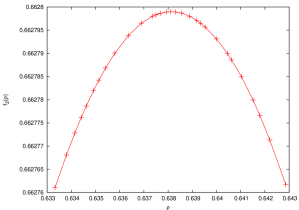
Figure 1: (Color online) The function of $f_{2}(\rho)$ in the region of $19/20\leq\rho\leq 9/14$. All data points use rational $\rho$, so no interpolation is used.

With the interpolated data for $a_{m,n}(\rho)$, we can locate $\rho^{*}$ and $f_{2}(\rho^{*})$ more accurately. As shown in Figures 2 and 3, we find that

$$0.662798972831<f_{2}(\rho^{*})<0.662798972845,$$

where the value of $f_{\infty,n}(\rho)$ for $n=16$ is used as the upper bounds, and that for $n=17$ as the lower bounds. From Figures 2, 3 and 4 we can locate $\rho^{*}$ as

$$0.63812310<\rho^{*}<0.63812312.$$

The values of $f_{\infty,n}(\rho)$ around $\rho^{*}$ are listed in Table VI. Inspection of the convergent rate of these data for even and odd values of $n$ suggests that for both sequences, the convergent rate is geometric. If we assume that

$$f_{\infty,n}(\rho)=f_{2}(\rho)-\alpha\eta^{n},$$ (19)

then the data points at $\rho=0.63812311$ of $n=12$, $14$, and $16$ can be used to obtain an extrapolated value of $f_{2}(\rho)=0.6627989728336$, while the data points of $n=13$, $15$, and $17$ give another extrapolation value $f_{2}(\rho)=0.6627989728341$. Together these two extrapolation values converge to $f_{2}(\rho^{*})=0.662798972834$, with $11$ correct digits.

We can also get the same conclusion graphically from Figure 3. By inspecting the pattern of the data points of different values of $n$ in the inset of Figure 3, we notice that the difference between the data points of $n=14$ and $n=16$ is bigger than the difference between $n=15$ and $n=17$. This indicates that the true value of $f_{2}(\rho^{*})$ lies closer to the data point of $n=17$ than the data point of $n=16$. From Figure 3 we are quite sure that the $11$-th digit of $f_{2}(\rho^{*})$ is $3$ instead of $4$, and the $12$-th digit is probably $4$, as indicated by the two extrapolation values mentioned above.

The value of $f_{2}(\rho^{*})$ is in excellent agreement with that reported in Ref. Friedland and Peled, 2005, which gives $9$ correct digits (Friedland and Peled also guess correctly the $10$-th digits as $8$). The value also agrees with that in Ref. Baxter, 1968, which gives $8$ correct digits Friedland and Peled (2005). The value of $\rho^{*}$ is exactly that of Baxter Baxter (1968).

By using field theoretical method, Samuel uses the following relation to transform the activity $x$ into a new variable $\omega$ Samuel (1980)

$$x=\frac{\omega}{(1-4\omega)^{2}}.$$ (20)

This relation is very close to the one used by Nagle Nagle (1966). By substituting this relation into Gaunt’s series expansions Gaunt (1969), Samuel obtained new series for various lattices, including the rectangular lattice (Eq. (5.12) of Ref. Samuel, 1980). The value of monomer-dimer constant in two-dimensional rectangular lattice can be calculated at $x=1$ by using his series as $0.66279914$. As we can see, this only gives five correct digits. Nagle used the following transform Nagle (1966)

$$x=\frac{\omega}{(1-3\omega)^{2}}.$$ (21)

By using Gaunt’s series, a value of $0.6627988$ is obtained, with six correct digits.

Table 4: The coefficient $c_{0}$ ($f_{\infty,n}(\rho)$) for different $n$ and $\rho$ on cylinder lattice strips $\infty\times n$ around $\rho^{*}$. The numbers in parentheses are the number of data points used in the fitting.

	0.63812309	0.63812310	0.63812311	0.63812312
1	0.470643631091106 (880)	0.470643628559868 (880)	0.470643626028629 (880)	0.470643623497390 (880)
2	0.683451694063943 (901)	0.683451695019491 (901)	0.683451695975038 (901)	0.683451696930585 (901)
3	0.659839104062378 (901)	0.659839103873019 (901)	0.659839103683659 (901)	0.659839103494298 (901)
4	0.663319985040839 (901)	0.663319985089007 (901)	0.663319985137175 (901)	0.663319985185343 (901)
5	0.662701144811933 (901)	0.662701144800592 (901)	0.662701144789251 (901)	0.662701144777910 (901)
6	0.662818978977777 (901)	0.662818978980627 (901)	0.662818978983477 (901)	0.662818978986327 (901)
7	0.662794695257766 (901)	0.662794695257048 (901)	0.662794695256327 (901)	0.662794695255611 (901)
8	0.662799924786436 (901)	0.662799924786622 (901)	0.662799924786807 (901)	0.662799924786992 (901)
9	0.662798754939549 (901)	0.662798754939501 (901)	0.662798754939453 (901)	0.662798754939404 (901)
10	0.662799023857733 (901)	0.662799023857746 (901)	0.662799023857758 (901)	0.662799023857771 (901)
11	0.662798960670265 (901)	0.662798960670262 (901)	0.662798960670259 (901)	0.662798960670256 (901)
12	0.662798975775941 (901)	0.662798975775943 (901)	0.662798975775944 (901)	0.662798975775944 (901)
13	0.662798972113454 (901)	0.662798972113453 (901)	0.662798972113445 (901)	0.662798972113451 (901)
14	0.662798973011855 (781)	0.662798973011855 (781)	0.662798973011855 (781)	0.662798973011855 (781)
15	0.662798972789303 (570)	0.662798972789304 (570)	0.662798972789304 (570)	0.662798972789303 (570)
16	0.662798972844882 (375)	0.662798972844882 (375)	0.662798972844883 (375)	0.662798972844883 (375)
17	0.662798972830869 (226)	0.662798972830871 (226)	0.662798972830870 (226)	0.662798972830869 (226)

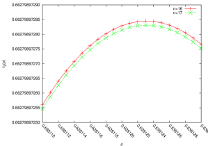
Figure 2: (Color online) The function of $f_{\infty,n}(\rho)$ in the region of $0.638110\leq\rho\leq 0.638130$ for $n=16$ (upper curve) and $n=17$ (lower curve).

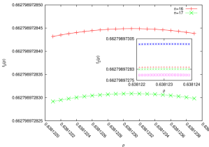
Figure 3: (Color online) The function of $f_{\infty,n}(\rho)$ in the region of $0.6381221\leq\rho\leq 0.6381239$ for $n=16$ (upper curve) and $n=17$ (lower curve). In the inset the data points from $n=14$ and $n=15$ are also shown. From top to bottom in the inset: $n=14$, $n=16$, $n=17$, and $n=15$.

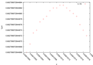
Figure 4: (Color online) The function of $f_{\infty,n}(\rho)$ in the region of $0.63812301\leq\rho\leq 0.63812319$ for $n=16$.

To conclude this section, we compare our results on the maximum of $f_{2}(\rho)$ with the approximate formulas of Chang Chang (1939) and Lin and Lai Lin and Lai (1994). The Chang’s approximate formula is given below

$$f_{2}^{C}(\rho)=-\frac{1}{2}[4\ln 4-(4-\rho)\ln(4-\rho)+\rho\ln\rho+2(1-\rho)\ln(1-\rho)-2\rho\ln 4],$$

which gives $\rho^{*}=0.634641$ and $f_{2}(\rho^{*})=0.661355$. The approximate formula of Lin and Lai is

$$f_{2}^{\text{LL}}(\rho)=-\frac{\rho}{2}\ln\frac{\rho}{2}-0.9030(1-\rho)\ln(1-\rho)-0.05645\rho$$

which gives $\rho^{*}=0.638057$ and $f_{2}(\rho^{*})=0.66282235$. Although the two formulas are quite simple, they give effective approximation with respect to $\rho^{*}$ and $f_{2}(\rho^{*})$.

VII Comparison with Baxter’s results

Using variational approach, Baxter calculated $h_{2}(x)$ (which is $\ln\kappa$ using his notation) and $\theta(x)$ (which is $2\rho$ by his notation) for different values of dimer activity $x$ ($s^{2}$ by his notation). By using Eqs. 28 and 29, we can compare our results with Baxter’s results in his Table II. For each of his data point at a dimer activity $x$, we calculate $f_{2}(\rho)$ with $\rho=\theta(x)$. Then his $h_{2}(x)$ is converted to $f_{2}^{B}(\rho)=h_{2}(x)-\frac{\rho}{2}\ln(x)$. The comparisons are shown in Table 5. It should be pointed out that in Baxter’s data, extrapolation is used for the sequence to obtain $\theta(x)$ and $h_{2}(x)$ when $x^{-1/2}$ is small ($x^{-1/2}<0.3$ for $h_{2}(x)$ and $x^{-1/2}<0.5$ for $\theta(x)$), while no extrapolation is used in our data: we only look at the digits that have been converged for $n=16$ and $n=17$. Although the extrapolation used in Baxter’s data makes the comparison less direct, we still see that the agreement is excellent. It seems that Baxter’s method converges faster for $\rho$ very close to $1$ (again the extrapolation factor has to be considered), and our method is more accurate when $\rho$ is not too close to $1$. As in Section IV, we only present the raw data here. If extrapolation is used, more correct digits can be obtained.

Table 5: Comparison with Baxter’s results. Numbers in square brackets indicate the next digits for $n=16$ (upper bound) and $n=17$ (lower bound).

$x^{-1/2}$	$\rho$	$f_{2}(\rho)$	$f_{2}^{B}(\rho)$
0.00	1.0	0.29[0..3]	0.291557
0.02	0.994176	0.319[2..8]	0.3194631
0.05	0.9836216	0.355[0..2]	0.35510683
0.10	0.96456376	0.4047[5..8]	0.404771005
0.20	0.924706050	0.4810[8..9]	0.4810887477
0.30	0.8846581140	0.536892[1..4]	0.5368922350
0.40	0.8453815864	0.5782845[2..9]	0.5782845477
0.50	0.8072764728	0.608814[3..4]	0.6088143934
0.60	0.7705280966	0.63085609[6..8]	0.6308560970
0.80	0.7013863228	0.655894637[3..5]	0.6558946374
1.00	0.6381231092	0.6627989728[3..4]	0.6627989726
1.50	0.5042633294	0.6349499289380[4..9]	0.6349499290
2.00	0.4006451804	0.5779686472227[1..4]	0.5779686472
2.50	0.3211782498	0.5140847735884[4..6]	0.5140847737
3.00	0.2603068980	0.4528361791290[7..9]	0.4528361790
3.50	0.2134739142	0.3978378948658[1..3]	0.3978378949
4.00	0.17715243204	0.3499573614350[0..2]	0.3499573615
4.50	0.14869898092	0.3088705309099[2..6]	0.3088705306
5.00	0.126162903820	0.273811439807[1..2]	0.2738114398

VIII High dimer density near close packing

It is well known that phase transition for the monomer-dimer model only occurs at $\rho=1$ Heilmann and Lieb (1972). Since the close-packed dimer system is at the critical point, it is interesting to investigate the behavior of the model when $\rho\rightarrow 1$. Using the similar computational procedure outlined before, the following results are obtained at high dimer density limit:

$$f_{\infty,n}(\rho)\sim f_{\infty,n}^{\text{lattice}}(1)+\begin{cases}-(1-\rho)\ln(1-\rho)&\text{$n$ is odd}\\ -\frac{1}{2}(1-\rho)\ln(1-\rho)&\text{$n$ is even}\\ \end{cases}$$ (22)

where $f_{\infty,n}^{\text{lattice}}(1)$ is the free energy of close-packed lattice with width $n$, and is given, based on the boundary condition, by Eq. 17 (cylinder lattices) or Eq. 18 (lattices with free boundary condition). Eq. 22 for $n=1$ is verified from the exact result as shown in Eq. 34. The result is also confirmed for other values of $n$ by using the Pemantle and Wilson asymptotic methods for multivariate generating function, as described in Section III. For space limitation these confirmations are not presented in this paper.

The dependence of the asymptotic form of $f_{\infty,n}(\rho)$ on the parity of the lattice width $n$ as shown in Eq. 22 reminds us of the results reported previously for monomer-dimer model with fixed number of monomers $v$ Kong (2006b), in which the coefficient of the logarithmic correction term of the free energy depends on the parity of the lattice width $n$. These two results are consistent with each other. If we substitute the relation $v=(1-\rho)mn$ into Eq. 22, we will get the logarithmic correction term with coefficient $v$ for odd $n$, and $v/2$ for even $n$. More discussions about this asymptotic form will be found in Section IX (Eq. 24).

We also investigate the behavior of $f_{2}(\rho)$ (for infinite lattice) as $\rho\rightarrow 1$. Since $f_{\infty,n}(\rho)$ does not converge fast enough as $\rho\rightarrow 1$ (Table IV), we use weighted average of $f_{\infty,16}(\rho)$ and $f_{\infty,17}(\rho)$ as an approximation of $f_{2}(\rho)$. The weights are calculated from the exact results at $\rho=1$. Fitting these data to the following function

$$f_{2}(\rho)=G/\pi+\frac{\gamma}{2}(1-\rho)\ln{(1-\rho)}+b_{1}(1-\rho),$$ (23)

we obtain $\gamma\approx 1.69775$ and $b_{1}\approx 0.427832$. No other reasonable form of functions other than Eq. (23) gives better fit. Including a term of $(1-\rho)^{2}$ in Eq. 23 leads to only slight changes in the values of $\gamma$ and $b_{1}$ The data and the fitting result are shown in Figure 5.

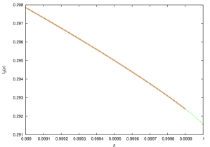
Figure 5: (Color online) Fitting result for $f_{2}(\rho)$ as $\rho\rightarrow 1$.

Using the equivalence between statistical ensembles discussed in Appendix A, we can relate our results with Gaunt’s series expansions Gaunt (1969). Plugging $f_{2}(\rho)$ as in Eq. 23 into $f(\rho)+\frac{\rho}{2}\ln(x)$ (see Eq. A), differentiating with respect to $\rho$, and solving for $\rho$, we obtain the average dimer density $\theta(x)$ at the activity $x$. Expressing $x$ as a function of $\theta$, we have

$$x=\frac{e^{2b_{1}-\gamma}}{(1-\theta)^{\gamma}}.$$

This is in the same form of Eq. (3.7) of Gaunt Gaunt (1969). If we put in the values of $\gamma$ and $b_{1}$, we can estimate the amplitude $A=\exp(2b_{1}-\gamma)=0.4308$. Gaunt obtains through series expansions $\gamma=1.73\pm 4$ and $A=0.3030\pm 4$, and conjectures that $\gamma=7/4$. Our results support the same functional form, and the numerical values are close to these obtained by Gaunt’s series analysis. As for the conjectured value of $\gamma$, the current data seem to indicate a value lower than $7/4$. In fact, the data presented here as well as theoretical arguments (not shown here) indicate that $\gamma=5/3$. More discussion on this constant can be found in the next Section.

IX Discussion

In Section III we show by computational methods that there is a logarithmic correction term in the free energy with a coefficient of $-1/2$. By introducing the newly developed Pemantle and Wilson asymptotic method, we give a theoretical explanation of this term. We also demonstrate that this term is not unique to the monomer-dimer model. Many statistical lattice models can be casted in the form of bivariate (or multivariate) generating functions, and when the two variables are proportional to each other so that the system is at a fixed “density”, we will expect such a universal logarithmic correction term with coefficient of $-1/2$. We anticipate more applications of this asymptotic method in statistical physics in the future.

The Pemantle and Wilson asymptotic method not only gives a nice explanation of the logarithmic correction term and its coefficient found by computational means, but also gives exact numerical values of $f_{\infty,n}(\rho)$ for small $n$ (the width of the lattice strips). These exact values can be used to check the accuracy of the computational method, as already mentioned in Section IV. In Section III we discuss how this can be done. The denominator $H(x,y)$ of the bivariate generating functions is derived from the characteristic function of the matrix $M_{n}$, and the size of $M_{n}$ is given by $u_{c}(n)$ in Section II for cylinder lattices, and in Ref. Kong, 2006a for lattices with free boundaries. For small $n$, the size of $M_{n}$ is small enough so that the characteristic function can be calculated symbolically. As $n$ increases, however, the size of $M_{n}$ increases exponentially: $u_{c}(17)=4112$ for cylinder lattice when $n=17$, and $u_{\text{fb}}(16)=32896$ when $n=16$. It is currently impractical to calculate the characteristic functions symbolically from matrices of such sizes to get $H(x,y)$ of the corresponding bivariate generating functions, so the Pemantle and Wilson method cannot be applied when the width of the lattice $n$ becomes larger. Even when $H(x,y)$ is available, it is of the order of thousands or higher, which will lead to instabilities in the numerical calculations. The computational method utilized here, however, can still give important and accurate data in these situations.

Previously we demonstrated that when the monomer number $v$ or the dimer number $s$ are fixed, there is also a logarithmic correction term in the free energy Kong (2006a, b). When the number of dimers is fixed (low dimer density limit), the coefficient of this term equal to the number of dimers. When the number of monomers is fixed (high dimer density limit), the coefficient, however, depends on the parity of the lattice width $n$: it equals to $v$ when $n$ is odd, and $v/2$ when $n$ is even. In this high dimer density limit, as $m\rightarrow\infty$, dimer density $\rho\rightarrow 1$. In this paper we focus on the situation where the dimer density is fixed, and find that again there is a logarithmic correction term, but this time its coefficient equals to $-1/2$ and does not depend on the parity of the lattice width. Why does the dependence of the coefficient on the parity of the lattice width disappear as dimer density $\rho\rightarrow 1$ and the lattice becomes almost completely covered by the dimers?

This seemingly paradoxical phenomenon can be explained as follows. When the number of monomer $v$ is fixed and as $m\rightarrow\infty$, if we can put $v=(1-\rho)mn$ into Eq. 22, then the term of $(1-\rho)\ln(1-\rho)$ leads to a term of $v\ln m/(mn)$ when $n$ is odd, and a term of $v\ln m/(2mn)$ when $n$ is even. At the same time, the logarithmic correction term with $-1/2$ as coefficient ($-\ln m/(2mn)$, the second term in Eq. 14), gets canceled out by the a term of $-\ln(1-\rho)/(2mn)$ from the third term in Eq. 14 as $m\rightarrow\infty$ and $\rho\rightarrow 1$. Putting Eqs. 14 and 22 together, we have for finite $n$, as $m\rightarrow\infty$ and $\rho\rightarrow 1$,

$$f_{m,n}(\rho)\sim f_{\infty,n}^{\text{lattice}}(1)+\left\{\begin{tabular}[]{l}$-(1-\rho)\ln(1-\rho)$\\ $-\frac{1}{2}(1-\rho)\ln(1-\rho)$\end{tabular}-\frac{1}{2mn}\ln m-\frac{1}{2mn}\ln(1-\rho)\quad\begin{tabular}[]{l}$n$ is odd\\ $n$ is even\\ \end{tabular}\right.$$ (24)

This expression can be checked with the explicit formulas for one-dimensional lattice, Eqs. 31 and 34. By using the relation $v=(1-\rho)mn$, we see from Eq. 24 that as $m\rightarrow\infty$, when the monomer number $v$ is fixed, the dependence of the logarithmic correction term on the parity of $n$ comes from the second term in the equation; the third and fourth terms cancel each other out. On the other hand when the dimer density $\rho$ is fixed, the only logarithmic correction term comes from the third term of Eq. 24, with coefficient $-1/2$.

As $n\rightarrow\infty$, $f_{2}(\rho)$ also has a term of $(1-\rho)\ln(1-\rho)$ (Eq. 23), whose coefficient is estimated as $-0.85$ (Section VIII). This value is closer to $-5/6=-0.83$ than to the conjectured value $-7/8=-0.875$ by Gaunt Gaunt (1969). Runnels’ result, however, seems to be closer to Gaunt’s result Runnels (1970). It should be recognized that, as pointed out previously Nagle (1966); Baxter (1968); Gaunt (1969); Runnels (1970); Samuel (1980) as well as in the present work, the convergence is poorest when the dimer density is near close packing. On the other hand, theoretical calculations underway (not shown here due to space limitation) indeed indicate that this coefficient of $(1-\rho)\ln(1-\rho)$ for the infinite lattice is $-5/6$, or equivalently, $\gamma=5/3$.

It is well known that there is a one to one correspondence between the Ising model in a rectangular lattice with zero magnetic field and a fully packed dimer model in a decorated lattice Kasteleyn (1963); Fisher (1966). By using a similar method Heilmann and Lieb (1972), it has been shown that the Ising model in a non-zero magnetic field, a well-known unsolved problem in statistical mechanics, can be mapped to a monomer-dimer model with dimer density $\rho<1$. The investigation of the monomer-dimer model near close packing is of interest within this context.

As mentioned in Section VI, several authors have applied field theoretic methods to analyze the monomer-dimer model (for example, Ref. Samuel, 1980). In such studies, the monomer-dimer problem is expressed as a fermionic field theory. For close-packed dimer model, the expression is a free field theory with quadratic action, which is exactly solvable as expected. For general monomer-dimer model, the expression is an interacting field theory with a quartic interaction term, and self-consistent Hartree approximation is used to improve the Feynman rules to derive the series expansions. The transforms that are obtained using these methods (such as Eq. 20, which is similar to Eq. 21) make the series expansions converge in the full range of the dimer activity. The accuracy of these calculations, however, is not comparable to the accuracy of the computational method reported here, possibly due to the limited length of the series expansion.

Appendix A Equivalence of statistical ensembles

Throughout the paper our focus is on the functions $f_{m,n}(\rho)$, $f_{\infty,n}(\rho)$, or $f_{2}(\rho)$ at a given dimer density $\rho$. These functions are in essence properties of the canonical ensemble. In this Appendix we make the connection between $f_{2}(\rho)$ and the functions of $\theta(x)$ and $h_{2}(x)$ as defined in Eqs. 2 and 4, which are properties of the grand canonical ensemble. The results are used in Section VIII to compare the results of near close packing dimer density with Gaunt’s series analysis, and in Section VII to compare our results with those of Baxter, whose calculations are carried out in terms of $\theta(x)$ and $h_{2}(x)$ Baxter (1968).

Suppose at $\rho=\rho^{*}$, the summand $a_{m,n}(\rho)x^{mn\rho/2}$ in Eq. 6 reaches its maximum. By using the standard thermodynamic equivalence between different statistical ensembles (Hill, 1987, Chap. 4), we have

$$h_{2}(x) =\lim_{m,n\rightarrow\infty}\frac{\ln Z_{m,n}(x)}{mn}$$

$$=\lim_{m,n\rightarrow\infty}\frac{\ln\sum_{0\leq\rho\leq 1}a_{m,n}(\rho)x^{mn\rho/2}}{mn}$$

$$=\lim_{m,n\rightarrow\infty}\frac{\ln a_{m,n}(\rho^{*})x^{mn\rho^{*}/2}}{mn}$$

$$=f_{2}(\rho^{*})+\frac{\rho^{*}}{2}\ln x.$$ (25)

In other words, if we define $F_{2}(\rho,x)=f_{2}(\rho)+\frac{\rho}{2}\ln x$, then

$$h_{2}(x)=\max_{0\leq\rho\leq 1}(f_{2}(\rho)+\frac{\rho}{2}\ln x)=\max_{0\leq\rho\leq 1}F_{2}(\rho,x).$$ (26)

As a special case, the monomer-dimer constant is the maximum of the function $f_{2}(\rho)$ by setting $x=1$

$$h_{2}=\max_{0\leq\rho\leq 1}f_{2}(\rho)=f_{2}(\rho^{*}).$$ (27)

The connection for the average dimer coverage can also be obtained by using Eqs. 2 and A as

$$\theta(x)=\lim_{m,n\rightarrow\infty}\theta_{m,n}(x)=\lim_{m,n\rightarrow\infty}\frac{2}{mn}\frac{\partial\ln Z_{m,n}(x)}{\partial\ln x}=\rho^{*}(x)$$ (28)

with the understanding that at $\rho^{*}$, $F_{2}(\rho,x)=f_{2}(\rho)+\frac{\rho}{2}\ln x$, not $f_{2}(\rho)$, reaches its maximum. Substituting Eq. 28 into Eq. A, we obtain

$$h_{2}(x)=f_{2}(\theta(x))+\frac{\theta(x)}{2}\ln x.$$ (29)

In Section VI, the excellent agreement of our result of $f_{2}(\rho^{*})$ with the result on $h_{2}$ of Friedland and Peled Friedland and Peled (2005) has already been demonstrated. In Ref. Friedland and Peled, 2005, what is calculated is actually $h_{2}$. Eq. 27 makes it possible to compare our result with that of Friedland and Peled. Eq. 27 is proved as a theorem for the specific monomer-dimer problem in Ref. Friedland and Peled, 2005 as Theorem 4.1.

Since there is an analytical solution to the one-dimensional lattice problem, Eqs. A and 28 can be confirmed for the one-dimensional lattice by explicit calculations, as shown in Appendix B.

Appendix B Explicit results for one-dimensional lattice

In this Appendix we summarize some exact results for the one-dimensional lattice ($n=1$) which are useful to compare and check the results for lattices with width $n>1$. When $n=1$, the problem is a special case of the so-called “parking problem” in one-dimensional lattice in which a $k$-mer covers $k$ consecutive lattice sites in a non-overlapping way. Various methods exist which lead to closed form solutions to the general case of interacting $k$-mers (for example, see Refs. Zasedatelev et al., 1971; Cera and Kong, 1996). For the monomer-dimer model, $k=2$ and there is no interaction between the dimers. The number of ways to put $s$ dimers in the $m\times 1$ lattice is known as

$$a_{m,1}(s)=\binom{m-s}{s}.$$ (30)

From this expression, in the next subsection we derive the asymptotic expression of the free energy by using the traditional method. As an illustration, later we also give an explicit demonstration of Pemantle and Wilson’s asymptotic method as it is applied to the bivariate generating function.

B.1 Canonical ensemble

From the explicit expression of Eq. 30, we can get the asymptotic expression of the free energy by using Stirling formula when $0<\rho<1$:

$$f_{m,1}(\rho)=\frac{\ln a_{m,1}(s)}{m}=f_{\infty,1}(\rho)-\frac{1}{2m}\ln m+\frac{1}{2m}\ln\frac{2-\rho}{\rho(1-\rho)}$$

$$+\sum_{j=1}^{\infty}\frac{2^{2j-2}B_{2j}}{j(2j-1)m^{2j}}\left[\frac{1}{(2-\rho)^{2j-1}}-\frac{1}{\rho^{2j-1}}-\frac{1}{2^{2j-1}(1-\rho)^{2j-1}}\right]$$ (31)

$$=f_{\infty,1}(\rho)-\frac{1}{2m}\ln(m+1)+\frac{1}{2m}\ln\frac{2-\rho}{\rho(1-\rho)}$$

$$+\sum_{j=1}^{\infty}\frac{1}{m^{2j}}\left[\frac{2^{2j-2}B_{2j}}{j(2j-1)}\left(\frac{1}{(2-\rho)^{2j-1}}-\frac{1}{\rho^{2j-1}}-\frac{1}{2^{2j-1}(1-\rho)^{2j-1}}\right)+\frac{1}{2(2j-1)}\right]-\sum_{j=1}^{\infty}\frac{1}{4jm^{2j+1}}$$ (32)

where

$$f_{\infty,1}(\rho)=(1-\frac{\rho}{2})\ln(1-\frac{\rho}{2})-\frac{\rho}{2}\ln\frac{\rho}{2}-(1-\rho)\ln(1-\rho)$$ (33)

and $B_{2j}$ are the Bernoulli numbers.

From Eqs. 31 or B.1 it is evident that for $n=1$, the coefficient of the logarithmic correction term is $\ell=-1/2$ for $0<\rho<1$.

The asymptotic expression of $f_{\infty,1}(\rho)$ (Eq. 33) at $\rho=1$ is given by

$$f_{\infty,1}(\rho)\sim-(1-\rho)\ln(1-\rho)-(\ln 2-1)(1-\rho)-\sum_{i=1}\frac{(1-\rho)^{2i+1}}{2i(2i+1)}$$ (34)

From this asymptotic expression we can see that the coefficient of $(1-\rho)\ln(1-\rho)$ is exactly $-1$, as in Eq. 22 for odd values of $n$. By combining Eqs. 31 and 34 together we confirm Eq. 24 for $n=1$ at high dimer density limit.

B.2 Grand canonical ensemble

In this section we calculate various quantities associated with the grand canonical ensemble. The configurational grand canonical partition function (Eq. 1) is

$$Z_{m,1}(x)=\sum_{s=0}^{m/2}\binom{m-s}{s}x^{s}$$

To get a closed form of $Z_{m,1}(x)$, we use the WZ method (Wilf-Zeilberger) Petkovšek et al. (1996) to get the following recurrence of $Z_{m,1}(x)$

$$xZ_{m,1}(x)+Z_{m+1,1}(x)-Z_{m+2,1}(x)=0,$$

from which we obtain the closed form solution as

$$Z_{m,1}(x)=\frac{1}{\sqrt{1+4x}}\left[\beta_{1}^{m+1}-\beta_{2}^{m+1}\right]$$ (35)

where

$$\beta_{1,2}=\frac{1\pm\sqrt{1+4x}}{2}.$$

To calculate $\theta(x)$ using Eq. 2, we need to evaluate the sum

$$S(m)=\sum_{s=0}^{m/2}\binom{m-s}{s}sx^{s}.$$

Again by using WZ method, we obtain the following recurrence for $S(m)$

$$(m+2)xS(m)+(m+1)S(m+1)-mS(m+2)=0.$$

To solve this recurrence, we use the generating function of $S(m)$: $G_{S}(z)=\sum_{m}S(m)z^{m}$, and get $G_{S}(z)$ from the recurrence as

$$G_{S}(z)=\frac{xz^{2}}{(1-z-xz^{2})^{2}}.$$

From $G_{S}(z)$ a closed form expression of $S(m)$ can be found as

$$S(m)=\frac{x}{1+4x}\left[(m-\frac{1}{\sqrt{1+4x}})\beta_{1}^{m}+(m+\frac{1}{\sqrt{1+4x}})\beta_{2}^{m}\right]$$ (36)

Substituting Eqs. 35 and 36 into Eq. 2, we obtain

$$\theta_{1}(x)=1-\frac{1}{\sqrt{1+4x}}$$ (37)

Using Eq. 35 we can calculate $h_{1}(x)$ as

$$h_{1}(x)=\lim_{m\rightarrow\infty}\frac{\ln Z_{m,1}(x)}{m}=\ln\frac{1+\sqrt{1+4x}}{2}$$ (38)

It is known that there are multiple methods to solve the one-dimensional lattice model. For example, transform matrix method can also be used Wu . In this case, the transform matrix is

$$T_{1}=\begin{bmatrix}0&x\\ 1&1\end{bmatrix},$$

whose eigenvalues are $\lambda_{1,2}=(1\pm\sqrt{1+4x})/2$. As $m\rightarrow\infty$, $Z_{m,1}(x)\sim\lambda_{1}^{m}$, so we obtain $h_{1}(x)$ as Eq. 38. From $\theta_{1}(x)=2\partial\ln\lambda_{1}/\partial\ln x$ we obtain Eq. 37.

B.3 Equivalence of statistical ensembles

The confirmation of the equivalence of ensembles for the special case of $x=1$ (Eq. 27) has been done in Ref. Friedland and Peled, 2005. Here we carry out the explicit calculations for the general case of arbitrary dimer activity $x$.

If we take the derivative of function $F_{1}(\rho,x)=f_{1}(\rho)+\frac{\rho}{2}\ln x$, where $f_{1}(\rho)=f_{\infty,1}(\rho)$ is given in Eq. 33, solve for $\rho$, and retain only the solution in $[0,1]$, we have

$$\rho^{*}=1-\frac{1}{\sqrt{1+4x}}$$

which is the same as Eq. 37. If we put the value of $\rho^{*}$ into $F_{1}(\rho,x)$, we obtain the maximum of $F_{1}(\rho^{*},x)$:

$$\max_{0\leq\rho\leq 1}(f_{1}(\rho)+\frac{\rho}{2}\ln x)=\ln\frac{1+\sqrt{1+4x}}{2}=h_{1}(x)$$

B.4 Application of Pemantle and Wilson asymptotic method to the bivariate generating function

The bivariate generating function of Eq, 13 can also be obtained in multiple ways, for example by direct summation of Eq. 35, or by using the characteristic function of $M_{1}$, or by using Eq. (23) of Ref. Cera and Kong, 1996 (by setting the interaction parameter $\sigma=1$ and the size of $k$-mer as 2), to get

$$F_{1}(x,y)=\frac{1}{1-y-xy^{2}}.$$ (39)

Here $G(x,y)=1$ and $H(x,y)=1-y-xy^{2}$. Solving the two equations in Eq. 12 we get $(x_{0},y_{0})$ as $(x_{0}=s(m-s)/(m-2s)^{2},y_{0}=(m-2s)/(m-s))$. Substituting $(x_{0},y_{0})$ into Eq. 11 we obtain

$$a_{m,1}\sim\frac{1}{\sqrt{2\pi}}(m-s)^{m-s+1/2}(m-2s)^{-m+2s-1/2}(s)^{-s-1/2}.$$

By putting $s=\rho m/2$, the first three terms of Eq. 31 are recovered, including the term of logarithmic correction $-\ln m/(2m)$. Higher order terms can also be obtained if more terms of the asymptotic expressions are used Pemantle and Wilson (2002).

References

- Fowler and Rushbrooke (1937) R. H. Fowler and G. S. Rushbrooke, Trans. Faraday Soc. 33, 1272 (1937).
- Kasteleyn (1961) P. W. Kasteleyn, Physica 27, 1209 (1961).
- Temperley and Fisher (1961) H. N. V. Temperley and M. E. Fisher, Philos. Mag. 6, 1061 (1961); M. E. Fisher, Phys. Rev. 124, 1664 (1961).
- Tzeng and Wu (2003) W.-J. Tzeng and F. Y. Wu, J. Stat. Phys. 110, 671 (2003).
- Wu (2006a) F. Y. Wu, Phys. Rev. E 74, 020104 (2006a); 74, 039907(E) (2006).
- Garey and Johnson (1979) M. R. Garey and D. S. Johnson, Computers and Intractability, A Guide to the Theory of NP-Completeness (W.H. Freeman and Company, New York, 1979); D. J. A. Welsh, Complexity: Knots, Colourings, and Counting, vol. 186 of London Mathematical Society Lecture Note Series (Cambridge University Press, 1993); S. Mertens, Computing in Science and Engineering 4, 31 (2002).
- Jerrum (1987) M. Jerrum, J. Stat. Phys. 48, 121 (1987); 59, 1087(E) (1990).
- Nagle (1966) J. F. Nagle, Phys. Rev. 152, 190 (1966).
- Gaunt (1969) D. Gaunt, Phys. Rev. 179, 174 (1969).
- Samuel (1980) S. Samuel, J. Math. Phys. 21, 2820 (1980).
- Bondy and Welsh (1966) J. Bondy and D. Welsh, Proc. Camb. Phil. Soc. Math. Phys. Sci. 62, 503 (1966); J. Hammersley, Proc. Camb. Phil. Soc. Math. Phys. Sci. 64, 455 (1968); J. Hammersley and V. Menon, J. Inst. Math. Appl. 6, 341 (1970); M. Ciucu, Duke Math. J 94, 1 (1998); P. H. Lundow, Disc. Math. 231, 321 (2001).
- Friedland and Peled (2005) S. Friedland and U. N. Peled, Adv. Appl. Math. 34, 486 (2005).
- Fisher and Stephenson (1963) M. E. Fisher and J. Stephenson, Phys. Rev. 132, 1411 (1963); R. E. Hartwig, J. Math. Phys. 7, 286 (1966).
- Heilmann and Lieb (1972) O. J. Heilmann and E. H. Lieb, Commun. Math. Phys. 25, 190 (1972).
- Gruber and Kunz (1971) C. Gruber and H. Kunz, Commun. Math. Phys. 22, 133 (1971).
- Ferdinand (1967) A. E. Ferdinand, J. Math. Phys. 8, 2332 (1967); N. S. Izmailian, K. B. Oganesyan, and C. K. Hu, Phys. Rev. E 67, 066114 (2003); N. S. Izmailian, V. B. Priezzhev, P. Ruelle, and C.-K. Hu, Phys. Rev. Lett. 95, 260602 (2005).
- Chang (1939) T. Chang, Proc. R. Soc. Series A 169, 512 (1939).
- Lin and Lai (1994) G. J. Lin and P. Y. Lai, Physica A 211, 465 (1994).
- Baxter (1968) R. J. Baxter, J. Math. Phys. 9, 650 (1968).
- Nemirovsky and Coutinho-Filho (1989) A. M. Nemirovsky and M. D. Coutinho-Filho, Phys. Rev. A 39, 3120 (1989); C. Kenyon, D. Randall, and A. Sinclair, J. Stat. Phys. 83, 637 (1996); I. Beichl, D. P. O’Leary, and F. Sullivan, Phys. Rev. E 64, 016701 (2001).
- Beichl and Sullivan (1999) I. Beichl and F. Sullivan, J. Comput. Phys. 149, 128 (1999).
- Kasteleyn (1963) P. W. Kasteleyn, J. Math. Phys. 4, 287 (1963).
- Fisher (1966) M. E. Fisher, J. Math. Phys. 7, 1776 (1966).
- Fan and Wu (1970) C. Fan and F. Wu, Phys. Rev. B 2, 723 (1970).
- McCoy and Wu (1973) B. M. McCoy and T. T. Wu, The two-dimensional Ising Model (Harvard University Press, Cambridge, Massachusetts, 1973).
- Pemantle and Wilson (2002) R. Pemantle and M. C. Wilson, J. Comb. Theory Ser. A 97, 129 (2002).
- Kong (1999) Y. Kong, J. Chem. Phys. 111, 4790 (1999).
- Kong (2006a) Y. Kong, Phys. Rev. E 73, 016106 (2006a).
- Kong (2006b) Y. Kong, Phys. Rev. E 74, 011102 (2006b).
- Granlund (2006) T. Granlund, GNU MP: The GNU Multiple Precision Arithmetic Library (2006), version 4.2, URL http://www.swox.com/gmp/.
- Calkin and Wilf (1998) N. J. Calkin and H. S. Wilf, SIAM J. Discrete Math. 11, 54 (1998).
- Runnels (1970) L. Runnels, J. Math. Phys. 11, 842 (1970).
- Stoer and Bulirsch (1992) J. Stoer and R. Bulirsch, Introduction to Numerical Analysis (Springer-Verlag, New York, USA, 1992), 2nd ed.
- Press et al. (1992) W. H. Press, S. A. Teukolsky, W. T. Vetterling, and B. P. Flannery, Numerical Recipes in C: The Art of Scientific Computing (Cambridge University Press, New York, NY, USA, 1992).
- Williams and Kelley (2004) T. Williams and C. Kelley, Gnuplot: An Interactive Plotting Program (2004), version 4.0, URL http://www.gnuplot.info.
- Marquart (1963) D. Marquart, J. Soc. Indust. Appl. Math. 11, 431 (1963).
- Hammersley (1966) J. Hammersley, in Research Papers in Statistics: Festschrift for J. Neyman, edited by F. David (Wiley, London, 1966), p. 125.
- Hill (1987) T. L. Hill, Statistical Mechanics : Principles and Applications (Dover Publications, New York, USA, 1987).
- Zasedatelev et al. (1971) A. Zasedatelev, G. Gurskii, and M. Volkenshtein, Mol. Biol. 5, 245 (1971); Y. Kong, J. Phys. Chem. B 105, 10111 (2001).
- Cera and Kong (1996) E. D. Cera and Y. Kong, Biophys. Chem. 61, 107 (1996).
- Petkovšek et al. (1996) M. Petkovšek, H. Wilf, and D. Zeilberger, A=B (AK Peters, Ltd., Wellesley, MA, USA, 1996).
- (42) F. Y. Wu, private communication.