The density-matrix renormalization group applied to transfer matrices: Static and dynamical properties of one-dimensional quantum systems at finite temperature

The density-matrix renormalization group (DMRG) applied to transfer matrices allows it to calculate static as well as dynamical properties of one-dimensional quantum systems at finite temperature in the thermodynamic limit. To this end the quantum system is mapped onto a two-dimensional classical system by a Trotter-Suzuki decomposition. Here we discuss two different mappings: The standard mapping onto a two-dimensional lattice with checkerboard structure as well as an alternative mapping introduced by two of us. For the classical system an appropriate quantum transfer matrix is defined which is then treated using a DMRG scheme. As applications, the calculation of thermodynamic properties for a spin-$1/2$ Heisenberg chain in a staggered magnetic field and the calculation of boundary contributions for open spin chains are discussed. Finally, we show how to obtain real time dynamics from a classical system with complex Boltzmann weights and present results for the autocorrelation function of the $XXZ$-chain.

1 Introduction

Several years after the invention of the DMRG method to study ground-state properties of one-dimensional (1D) quantum systems WhiteDMRG , Nishino showed that the same method can also be applied to the transfer matrix of a two-dimensional (2D) classical system hence allowing to calculate its partition function at finite temperature Nishino . The same idea can also be used to calculate the thermodynamic properties of a 1D quantum system after mapping it to a 2D classical one with the help of a Trotter-Suzuki decomposition Trotter ; Suzuki1 ; Suzuki2 . Bursill et. al. BursillXiang then presented the first application but the density matrix chosen in this work to truncate the Hilbert space was not optimal so that the true potential of this new numerical method was not immediately clear. This changed when Wang and Xiang WangXiang and Shibata Shibata presented an improved algorithm and showed that the density-matrix renormalization group applied to transfer matrices (which we will denote as TMRG from hereon) is indeed a serious competitor to other numerical methods as for example Quantum-Monte-Carlo (QMC). Since then, the TMRG method has been successfully applied to a number of systems including various spin chains, the Kondo lattice model, the $t-J$ chain and ladder and also spin-orbital models EggertRommer ; Raupach ; RiceTroyer ; SirkerKhaliullin ; SirkerSu4 ; MutouShibata ; SirkerKluemperEPL ; SirkerKluemperPRB ; NaefWang .

The main advantage of the TMRG algorithm is that the thermodynamic limit can be performed exactly thus avoiding an extrapolation in system size. Furthermore, there are no statistical errors and results can be obtained with an accuracy comparable to $T=0$ DMRG calculations. Similar to the $T=0$ DMRG algorithms, the method is best suited for 1D systems with short range interactions. These systems can, however, be either bosonic or fermionic because no negative sign problem as in QMC exists. Most important, there are two areas where TMRG seems to have an edge over any other numerical methods known today. These are: (1) Impurity or boundary contributions, and (2) real-time dynamics at finite temperature. As first shown by Rommer and Eggert RommerEggert , the TMRG method allows it to separate an impurity or boundary contribution from the bulk part thus giving direct access to quantities which are of order $\mathcal{O}(1/L)$ compared to the $\mathcal{O}(1)$ bulk contribution (here $L$ denotes the length of the system). We will discuss this in more detail in section 5. Calculating numerically the dynamical properties for large or even infinite 1D quantum systems constitutes a particularly difficult problem because QMC and TMRG algorithms can usually only deal with imaginary-time correlation functions. The analytical continuation of numerical data is, however, an ill-posed problem putting severe constraints on the reliability of results obtained this way. Very recently, two of us have presented a modified TMRG algorithm which allows for the direct calculation of real-time correlations SirkerKluemperDTMRG . This new algorithm will be discussed in section 6.

Before coming to these more recent developments we will discuss the definition of an appropriate quantum transfer matrix for the classical system in section 2 and describe how the DMRG algorithm is applied to this object in section 3. Here we will follow in parts the article by Wang and Xiang in Peschel but, at the same time, also discuss an alternative Trotter-Suzuki decomposition SirkerKluemperEPL ; SirkerKluemperPRB .

2 Quantum transfer matrix theory

The TMRG method is based on a Trotter-Suzuki decomposition of the partition function, mapping a 1D quantum system to a 2D classical one Trotter ; Suzuki1 ; Suzuki2 . In the following, we discuss both the standard mapping introduced by Suzuki Suzuki2 as well as an alternative one SirkerKluemperEPL ; SirkerKluemperPRB starting from an arbitrary Hamiltonian $H$ of a 1D quantum system with length $L$, periodic boundary conditions and nearest neighbor interaction

$$H=\sum_{i=1}^{L}h_{i,i+1}\;.$$ (1)

The standard mapping, widely used in QMC and TMRG calculations, is described in detail in Peschel . Therefore we only summarize it briefly here. First, the Hamiltonian is decomposed into two parts, $H=H_{e}+H_{o}$, where each part is a sum of commuting terms. Here $H_{e}$ ($H_{o}$) contains the interactions $h_{i,i+1}$ with $i$ even (odd). By discretizing the imaginary time, the partition function becomes

$$Z=\mbox{Tr}\;\mbox{e}^{-\beta H}=\lim_{M\to\infty}\mbox{Tr}\left\{\left[\mbox{e}^{-\epsilon H_{e}}\mbox{e}^{-\epsilon H_{o}}\right]^{M}\right\}$$ (2)

with $\epsilon=\beta/M$, $\beta$ being the inverse temperature and $M$ an integer (the so called Trotter number). By inserting $2M$ times a representation of the identity operator, the partition function is expressed by a product of local Boltzmann weights

$$\tau_{k,k+1}^{i,i+1}=\left<s_{k}^{i}s_{k}^{i+1}\right|\mbox{e}^{-\epsilon H_{e,o}}\left|s_{k+1}^{i}s_{k+1}^{i+1}\right>\;,$$ (3)

denoted in a graphical language by a shaded plaquette (see Fig. 1). The subscripts $i$ and $k$ represent the spin coordinates in the space and the Trotter (imaginary time) directions, respectively. A column-to-column transfer matrix $\mathcal{T}_{M}$, the so called quantum transfer matrix (QTM), can now be defined using these local Boltzmann weights

$$\mathcal{T}_{M}=\left(\tau_{1,2}\tau_{3,4}\ldots\tau_{2M-1,2M}\right)\left(\tau_{2,3}\tau_{4,5}\ldots\tau_{2M,1}\right)\;.$$ (4)

and is shown in the left part of Fig. 1. The partition function is then simply given by

$$Z=\mbox{Tr}\;\mathcal{T}_{M}^{L/2}\;.$$ (5)

The disadvantage of this Trotter-Suzuki mapping to a 2D lattice with checkerboard structure is that the QTM is two columns wide. This increases the amount of memory necessary to store it and also complicates the calculation of correlation functions.

Alternatively, the partition function can also be expressed by SirkerKluemperEPL ; SirkerKluemperPRB

$$Z=\lim_{M\to\infty}\mbox{Tr}\left\{\left[\mathcal{T}_{1}(\epsilon)\mathcal{T}_{2}(\epsilon)\right]^{M/2}\right\}\;,$$ (6)

with $\mathcal{T}_{1,2}(\epsilon)=T_{R,L}\exp[-\epsilon H+\mathcal{O}(\epsilon^{2})]$. Here, $T_{R,L}$ are the right- and left-shift operators, respectively. The obtained classical lattice has alternating rows and additional points in a mathematical auxiliary space. Its main advantage is that it allows to formulate a QTM which is only one column wide (see right part of Fig. 1).

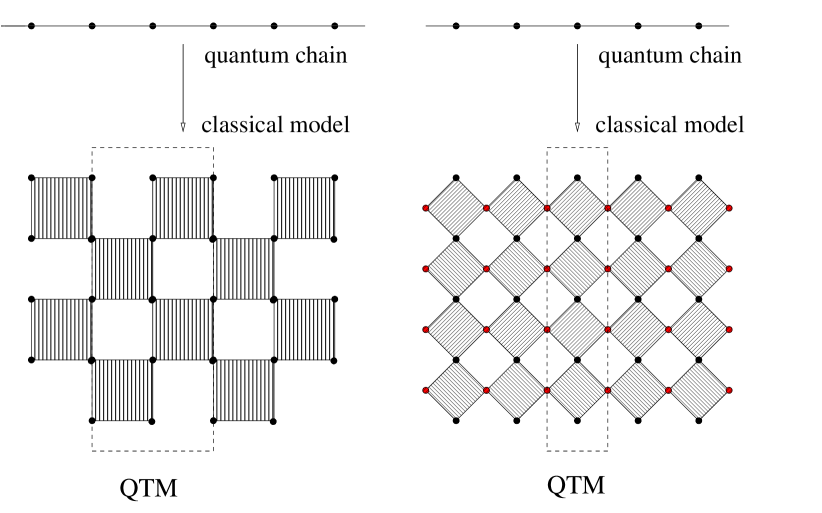
Figure 1: The left part shows the standard Trotter-Suzuki mapping of the 1D quantum chain to a 2D classical model with checkerboard structure where the vertical direction corresponds to imaginary time. The QTM is two-column wide. The right part shows the alternative mapping. Here, the QTM is only one column wide.

The derivation of this QTM is completely analogous to the standard one, even the shaded plaquettes denote the same Boltzmann weight. Here, however, these weights are rotated by 45⁰ clockwise and anti-clockwise in an alternating fashion from row to row. Using this transfer matrix, $\widetilde{\mathcal{T}}_{M}$, the partition function is given by $Z=\mbox{Tr}\;\widetilde{\mathcal{T}}_{M}^{L}$.

2.1 Physical properties in the thermodynamic limit

The reason why this transfer matrix formalism is extremely useful for numerical calculations has to do with the eigenspectrum of the QTM. At infinite temperature it is easy to show SirkerDiss that the largest eigenvalue of the QTM $\mathcal{T}_{M}$ ($\widetilde{\mathcal{T}}_{M}$) is given by $S^{2}$ ($S$) and all other eigenvalues are zero. Here $S$ denotes the number of degrees of freedom of the physical system per lattice site. Decreasing the temperature, the gap between the leading eigenvalue $\Lambda_{0}$ and next-leading eigenvalues $\Lambda_{n}$ ($n>0$) of the transfer matrix shrinks. The ratio between $\Lambda_{0}$ and each of the other eigenvalues $\Lambda_{n}$, however, defines a correlation length $1/\xi_{n}=\ln|\Lambda_{0}/\Lambda_{n}|$ Peschel ; SirkerDiss . Because a 1D quantum system cannot order at finite temperature, any correlation length $\xi_{n}$ will stay finite for $T>0$, i.e., the gap between the leading and any next-leading eigenvalue stays finite. Therefore the calculation of the free energy in the thermodynamic limit boils down to the calculation of the largest eigenvalue $\Lambda_{0}$ of the QTM

$$f = -\lim_{L\to\infty}\frac{1}{\beta L}\ln Z=-\lim_{L\to\infty}\lim_{\epsilon\to 0}\frac{1}{\beta L}\ln\mbox{Tr}\,\widetilde{\mathcal{T}}_{M}^{L}$$ (7)

$$= -\lim_{\epsilon\to 0}\lim_{L\to\infty}\frac{1}{\beta L}\ln\bigg{\{}\Lambda_{0}^{L}\bigg{[}1+\sum_{l>1}\underbrace{\left(\Lambda_{l}/\Lambda_{0}\right)^{L}}_{\stackrel{{\scriptstyle L\to\infty}}{{\longrightarrow 0}}}\bigg{]}\bigg{\}}$$

$$= -\lim_{\epsilon\to 0}\frac{\ln\Lambda_{0}}{\beta}\;.$$

Here the interchangeability of the limits $L\rightarrow\infty$ and $\epsilon\rightarrow 0$ has been used Suzuki2 . Local expectation values and static two-point correlation functions can be calculated in a similar fashion (see e.g. Peschel and SirkerDiss ). In the next section, we are going to show how the eigenvalues of the QTM are computed by means of the density matrix renormalization group. This is possible since the transfer matrices are built from local objects. Instead of sums of local objects we are dealing with products, but this is not essential to the numerical method. However, there are a few important differences in treating transfer matrices instead of Hamiltonians. At first sight, these differences look technical, but at closer inspection they reveal a physical core.

The QTMs as introduced above are real valued, but not symmetric. This is not a serious drawback for numerical computations, but certainly inconvenient. So the first question that arises is whether the transfer matrices can be symmetrized. Unfortunately, this is not the case. If the transfer matrix were replaceable by a real symmetric (or a hermitean) matrix all eigenvalues would be real and the ratios of next-leading eigenvalues to the leading eigenvalue would be real, positive or negative. Hence all correlation functions would show commensurability with the lattice. However, we know that a generic quantum system at sufficiently low temperatures yields incommensurate oscillations with wave vectors being multiples of the Fermi vector taking rather arbitrary values.

Therefore we know that the spectrum of a QTM must consist of real eigenvalues or of complex eigenvalues organized in complex conjugate pairs. This opens the possibility to understand the QTM as a normal matrix upon a suitable choice of the underlying scalar product. Unfortunately, the above introduced matrices are not normal with respect to standard scalar products, i.e. we do not have $[\widetilde{\mathcal{T}}_{M},\widetilde{\mathcal{T}}_{M}^{\dagger}]=0$.

3 The Method - DMRG algorithm for the QTM

Next, we describe how to increase the length of the transfer matrix in imaginary time, i.e. the inverse temperature, by successive DMRG steps. Like in the ordinary DMRG, we first divide the QTM into two parts, the system $S$ and the environment block $E$. Using the QTM, $\widetilde{\mathcal{T}}_{M}$, the density matrix is defined by

$$\rho=\widetilde{\mathcal{T}}_{M}^{L}\;,$$ (8)

which reduces to $\rho=\left|\Psi_{0}^{R}\right>\left<\Psi_{0}^{L}\right|$ up to a normalization constant in the thermodynamic limit. As in the zero temperature DMRG algorithm, a reduced density matrix $\rho_{S}$ is obtained by taking a partial trace over the environment

$$\rho_{S}=\mbox{Tr}_{E}\{\left|\Psi_{0}^{R}\right>\left<\Psi_{0}^{L}\right|\}\;.$$ (9)

Note that this matrix is real but non-symmetric, which complicates its numerical diagonalization. It also allows for complex conjugated pairs of eigenvalues which have to be treated separately (see SirkerDiss for details).

In actual computations, the Trotter-Suzuki parameter $\epsilon$ is fixed. Therefore the temperature $T\sim 1/\epsilon M$ is decreased by an iterative algorithm $M\to M+1$. In the following, the blocks of the QTM, $\widetilde{\mathcal{T}}_{M}$, are shown in a $90^{\circ}$-rotated view.

1. First we construct the initial system block $\Gamma$ consisting of $M$ plaquettes so that $S^{M}\leq N<S^{M+1}$, where $S$ is the dimension of the local Hilbert space and $N$ is the number of states which we want to keep.

   

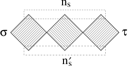
   Figure 2: The system block $\Gamma$. The plaquettes are connected by a summation over the adjacent corner spins.

   $n_{s},n_{s}^{\prime}$ are block-spin variables and contain $\widetilde{N}=S^{M}$ states. The $S^{2}\cdot\widetilde{N}^{2}$-dimensional array $\Gamma(\sigma,n_{s},\tau,n_{s}^{\prime})$ is stored.

2. The enlarged system block $\widetilde{\Gamma}(\sigma,n_{s},s_{2},\tau,s_{2}^{\prime},n_{s}^{\prime})$, a $S^{4}\cdot\widetilde{N}^{2}$-dimensional array, is formed by adding a plaquette to the system block. If $h_{i,i+1}$ is real and translationally invariant, the environment block can be constructed by a $180^{\circ}$-rotation and a following inversion of the system block. Otherwise the environment block has to be treated separately like the system block. Together both blocks form the superblock (see Fig. 3).

   

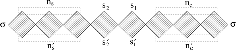
   Figure 3: The superblock is closed periodically by a summation over all $\sigma$ states.

3. The leading eigenvalue $\Lambda_{0}$ and the corresponding left and right eigenstates

   $$\left<\Psi_{0}^{L}\right|=\Psi^{L}(s_{1},n_{s},s_{2},n_{e})\;,\;\left|\Psi_{0}^{R}\right>=\Psi^{R}(s_{1}^{\prime},n_{s}^{\prime},s_{2}^{\prime},n_{e}^{\prime})$$ (10)

   are calculated and normalized $\langle\Psi_{0}^{L}|\Psi_{0}^{R}\rangle=1$. Now thermodynamic quantities can be evaluated at the temperature $T=1/(2\epsilon(M+1))$.

4. A reduced density matrix is calculated by performing the trace over the environment

   $$\rho_{s}(n_{s}^{\prime},s^{\prime}_{2}|n_{s},s_{2}) = \sum_{s1,n_{e}}\left|\Psi_{0}^{R}\right>\left<\Psi_{0}^{L}\right|$$

   $$= \sum_{s1,n_{e}}\Psi^{R}(s_{1},n_{s}^{\prime},s_{2}^{\prime},n_{e})\Psi^{L}(s_{1},n_{s},s_{2},n_{e})$$

   and the complete spectrum is computed. A $N\times(S\cdot\widetilde{N})$-matrix $V^{L}(\widetilde{n}_{s}|n_{s},s_{2})$ ($V^{R}(\widetilde{n}_{s}^{\prime}|n_{s}^{\prime},s_{2}^{\prime})$) is constructed using the left (right) eigenstates belonging to the $N$ largest eigenvalues, where $\widetilde{n}_{s}$ ($\widetilde{n}_{s}^{\prime}$) is a new renormalized block-spin variable with only $N$ possible values.

5. Using $V^{L}$ and $V^{R}$ the system block is renormalized.

   

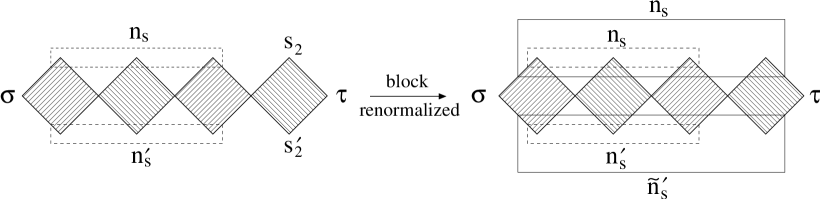
   Figure 4: The renormalization step for the system block.

   The renormalization is given by

   $$\Gamma(\sigma,\widetilde{n}_{s},\tau,\widetilde{n}_{s}^{\prime})=\sum_{n_{s},s_{2}}\sum_{n_{s}^{\prime},s_{2}^{\prime}}V^{L}(\widetilde{n}_{s}|n_{s},s_{2})\widetilde{\Gamma}(\sigma,n_{s},s_{2},\tau,s_{2}^{\prime},n_{s}^{\prime})V^{R}(\widetilde{n}_{s}^{\prime}|n_{s}^{\prime},s_{2}^{\prime})\;.$$ (12)

Now the algorithm is repeated starting with step 2 using the new system block. However, the block-spin variables can now take $N$ instead of $\widetilde{N}$ values.

4 An example: The spin-$1/2$ Heisenberg chain with staggered and uniform magnetic fields

As example, we show here results for the magnetization of a spin-$1/2$ Heisenberg chain subject to a staggered magnetic field $h_{s}$ and a uniform field $h_{u}=g\mu_{B}H/J$

$$\mathcal{H}=J\sum_{i}\left[\mathbf{S}_{i}\mathbf{S}_{i+1}-h_{u}S_{i}^{z}-(-1)^{i}h_{s}S_{i}^{x}\right]\;,$$ (13)

where $H$ is the external uniform magnetic field and $g$ the Landé factor. An effective staggered magnetic field is realized in spin-chain compounds as for example copper pyrimidine dinitrate (CuPM) or copper benzoate if an external uniform magnetic field $H$ is applied OshikawaAffleck . For CuPM the magnetization as a function of applied magnetic field $H$ has been measured experimentally. In Fig. 5 the excellent agreement between these experimental and TMRG data at a temperature $T=1.6$ K with a magnetic field applied along the $c^{\prime\prime}$ axis is shown. Along the $c^{\prime\prime}$ axis the effect due to the induced staggered field is largest (see Glocke for more details). Note that at low magnetic fields the TMRG data describe the experiment more accurately than the exact diagonalization (ED) data, because there are no finite size effects (see inset (a) of Fig. 5).

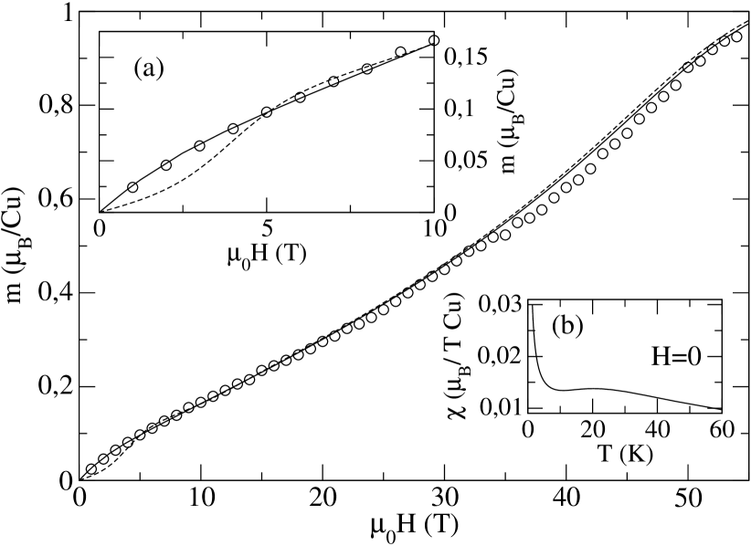
Figure 5: TMRG data (solid line) and experimental magnetization curves (circles) for CuPM at a temperature $T=1.6$ K with the magnetic field applied along the $c^{\prime\prime}$ axis. For comparison ED data for a system of $16$ sites and $T=0$ are shown (dashed lines). Here $J/k_{B}=36.5$ K, $h_{u}=g\mu_{B}H/J$, $h_{s}=0.11\,h_{u}$ and $g=2.19$. Inset (a): Magnetization for small magnetic fields. Inset (b): Susceptibility as a function of temperature $T$ at $H=0$ calculated by TMRG.

For a magnetic field $H$ applied along the $c^{\prime\prime}$ axis a gap, $\Delta\propto H^{2/3}$, is induced with multiplicative logarithmic corrections. For $H\to 0$ and low $T$ the susceptibility diverges $\chi\sim 1/T$ because of the staggered part OshikawaAffleckCUB (see inset (b) of Fig. 5).

5 Impurity and boundary contributions

In recent years much interest has focused on the question how impurities and boundaries influence the physical properties of spin chains EggertAffleck92 ; FujimotoEggert ; SirkerBortzJSTAT ; FurusakiHikihara ; SirkerLaflorencie . The doping level $p$ defines an average chain length $\bar{L}=1/p-1$ and impurity or boundary contributions are of order $\sim\mathcal{O}(1/\bar{L})$ compared to the bulk. This makes it very difficult to separate these contributions from finite size corrections if numerical data for finite systems (e.g. from QMC calculations) are used. TMRG, on the other hand, allows to study directly impurities embedded into an infinite chain RommerEggert . We will discuss here only the simplest case that a single bond or a single site is different from the rest. The partition function is then given by

$$Z=\mbox{Tr}\left(\widetilde{\mathcal{T}}_{M}^{L-1}\mathcal{T}_{imp}\right)\;,$$ (14)

where $\mathcal{T}_{imp}$ is the QTM describing the site impurity or the modified bond. In the thermodynamic limit the total free energy then becomes

$$F=-T\ln Z=Lf_{\mbox{\tiny bulk}}+F_{\mbox{\tiny imp}}=-LT\ln\Lambda_{0}-T\ln(\lambda_{imp}/\Lambda_{0})\;,$$ (15)

with $\Lambda_{0}$ being the largest eigenvalue of the QTM, $\widetilde{\mathcal{T}}_{M}$, and $\lambda_{imp}=\langle\Psi^{L}_{0}|\mathcal{T}_{imp}|\Psi^{R}_{0}\rangle$.

As example, we want to consider a semi-infinite spin-$1/2$ $XXZ$-chain with an open boundary. In this case translational invariance is broken and field theory predicts Friedel-type oscillations in the local magnetization $\langle S^{z}(r)\rangle$ and susceptibility $\chi(r)=\partial\langle S^{z}(r)\rangle/\partial h$ near the boundary EggertAffleck95 ; BortzSirker . Using the TMRG method the local magnetization can be calculated by

$$\langle S^{z}(r)\rangle=\frac{\langle\Psi_{L}^{0}|\widetilde{\mathcal{T}}(S^{z})\widetilde{\mathcal{T}}^{r-1}\mathcal{T}_{\mbox{\tiny imp}}|\Psi_{R}^{0}\rangle}{\Lambda_{0}^{r}\lambda_{imp}}\;,$$ (16)

where $\widetilde{\mathcal{T}}(S^{z})$ is the transfer matrix with the operator $S^{z}$ included and $\mathcal{T}_{\mbox{\tiny imp}}$ is the transfer matrix corresponding to the bond with zero exchange coupling. Hence $\mathcal{T}_{\mbox{\tiny imp}}|\Psi_{R}^{0}\rangle$ is nothing but the state describing the open boundary at the right.

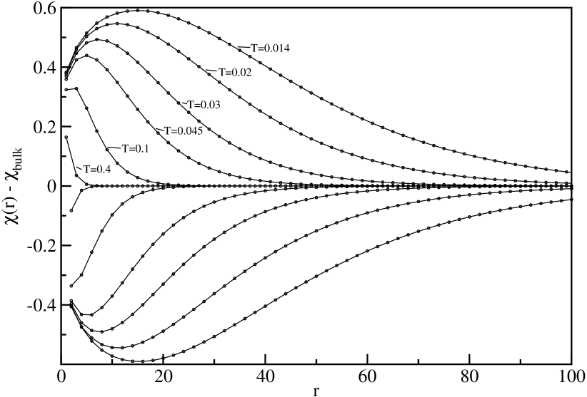
Figure 6: Susceptibility profile for $\Delta=0.6$ and different temperatures $T$. $N=240$ states have been kept in the DMRG algorithm. The lines are a guide to the eye.

In Fig. 6 the susceptibility profile as a function of the distance $r$ from the boundary for various temperatures as obtained by TMRG calculations BortzSirker is shown. For more details the reader is referred to RommerEggert and BortzSirker .

6 Real time dynamics

Finally, we want to discuss a very recent development in the TMRG method. The Trotter-Suzuki decomposition of a 1D quantum system yields a 2D classical model with one axis corresponding to imaginary time (inverse temperature). It is therefore straightforward to calculate imaginary-time correlation functions (CFs). Although the results for the imaginary-time CFs obtained by TMRG are very accurate, the results for real-times (real-frequencies) involve errors of unknown magnitude because the analytical continuation poses an ill-conditioned problem. In practice, the maximum entropy method is the most efficient way to obtain spectral functions from TMRG data. The combination of TMRG and maximum entropy has been used to calculate spectral functions for the $XXZ$-chain NaefWang and the Kondo-lattice model MutouShibata . However, it is in principle impossible to say how reliable these results are because of the afore mentioned problems connected with the analytical continuation of numerical data. It is therefore desirable to avoid this step completely and to calculate real-time correlation functions directly.

A TMRG algorithm to do this has recently been proposed by two of us SirkerKluemperDTMRG . Starting point is an arbitrary two-point CF for an operator $\hat{O}_{r}(t)$ at site $r$ and time $t$

$$\langle\hat{O}_{r}(t)\hat{O}_{0}(0)\rangle=\frac{\mbox{Tr}\left(\hat{O}_{r}(t)\hat{O}_{0}(0)\mbox{e}^{-\beta H}\right)}{\mbox{Tr}\left(\mbox{e}^{-\beta H}\right)}=\frac{\mbox{Tr}\left(\mbox{e}^{-\beta H/2}\mbox{e}^{itH}\hat{O}_{r}\mbox{e}^{-itH}\hat{O}_{0}\mbox{e}^{-\beta H/2}\right)}{\mbox{Tr}\left(\mbox{e}^{-\beta H/2}\mbox{e}^{itH}\mbox{e}^{-itH}\mbox{e}^{-\beta H/2}\right)}\;.$$ (17)

Here we have used the cyclic invariance of the trace and have written the denominator in analogy to the numerator. In the following we will use the standard Trotter-Suzuki decomposition leading to a two-dimensional checkerboard model.

The crucial step in our approach to calculate real-time dynamics directly is to introduce a second Trotter-Suzuki decomposition of $\exp(-\mbox{i}\delta H)$ with $\delta=t/N$ in addition to the usual one for the partition function described in section 2. We can then define a column-to-column transfer matrix

$$\mathcal{T}_{2N,M}=(\tau_{1,2}\tau_{3,4}\cdots\tau_{2M-1,2M})(\tau_{2,3}\tau_{4,5}\cdots\tau_{2M,2M+1})$$

$$(\bar{v}_{2M+1,2M+2}\cdots\bar{v}_{2M+2N-1,2M+2N})(\bar{v}_{2M+2,2M+3}\cdots\bar{v}_{2M+2N,2M+2N+1})$$

$$(v_{2M+2N+1,2M+2N+2}\cdots v_{2M+4N-1,2M+4N})(v_{2M+2N+2,2M+2N+3}\cdots v_{2M+4N,1})$$

where the local transfer matrices have matrix elements

$$\tau(s_{k}^{i}s_{k}^{i+1}|s_{k+1}^{i}s_{k+1}^{i+1}) = \langle s_{k}^{i}s_{k}^{i+1}|\mbox{e}^{-\epsilon h_{i,i+1}}|s_{k+1}^{i}s_{k+1}^{i+1}\rangle$$ (19)

$$v(s_{l}^{i}s_{l}^{i+1}|s_{l+1}^{i}s_{l+1}^{i+1}) = \langle s_{l}^{i}s_{l}^{i+1}|\mbox{e}^{-i\delta h_{i,i+1}}|s_{l+1}^{i}s_{l+1}^{i+1}\rangle\;$$

and $\bar{v}$ is the complex conjugate. Here $i=1,\cdots,L$ is the lattice site, $k=1,\cdots,2M$ ($l=1,\cdots,2N$) the index of the imaginary time (real time) slices and $s_{k(l)}^{i}$ denotes a local basis. The denominator in Eq. (17) can then be represented by $\mbox{Tr}(\mathcal{T}_{2N,M}^{L/2})$ where $N,M,L\rightarrow\infty$. A similar path-integral representation holds for the numerator in (17). Here we have to introduce an additional modified transfer matrix $\mathcal{T}_{2N,M}(\hat{O})$ which contains the operator $\hat{O}$ at the appropriate position. For $r>1$ we find

$$\langle\hat{O}_{r}(t)\hat{O}_{0}(0)\rangle = \lim_{N,M\rightarrow\infty}\lim_{L\rightarrow\infty}\frac{\mbox{Tr}(\mathcal{T}(\hat{O})\mathcal{T}^{[r/2]-1}\mathcal{T}(\hat{O})\mathcal{T}^{L/2-[r/2]-1})}{\mbox{Tr}(\mathcal{T}^{L/2})}$$ (20)

$$= \lim_{N,M\rightarrow\infty}\frac{\langle\Psi^{L}_{0}|\mathcal{T}(\hat{O})\mathcal{T}^{[r/2]-1}\mathcal{T}(\hat{O})|\Psi^{R}_{0}\rangle}{\Lambda_{0}^{[r/2]+1}\langle\Psi^{L}_{0}|\Psi^{R}_{0}\rangle}\;.$$

Here $[r/2]$ denotes the first integer smaller than or equal to $r/2$ and we have set $\mathcal{T}\equiv\mathcal{T}_{2N,M}$. A graphical representation of the transfer matrices appearing in the numerator of Eq. (20) is shown in Fig. 7.

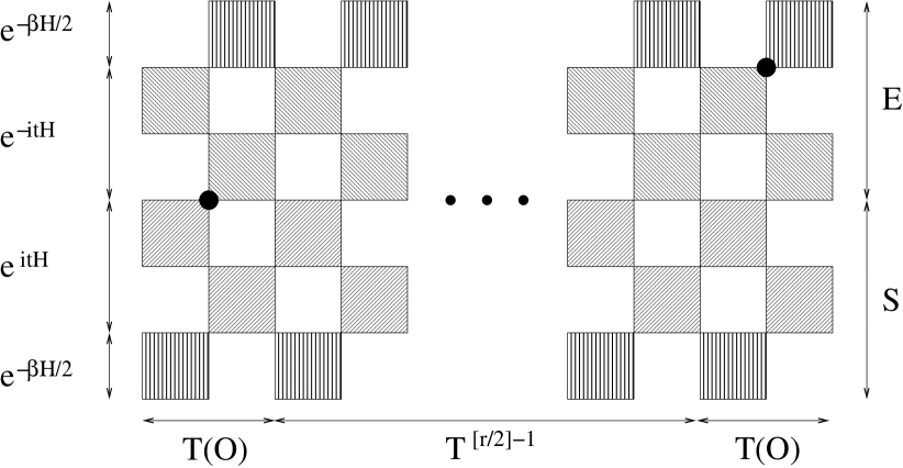
Figure 7: Transfer matrices appearing in the numerator of Eq. (20) for $r>1$ with $r$ even. The 2 black dots denote the operator $\mathcal{O}$. $\mathcal{T},\mathcal{T}(O)$ consist of three parts: A part representing $\exp(-\beta H)$ (vertically striped plaquettes), another for $\exp(\mbox{i}tH)$ (stripes from lower left to upper right) and a third part describing $\exp(-\mbox{i}tH)$ (upper left to lower right). $\mathcal{T},\mathcal{T}(O)$ are split into system ($S$) and environment ($E$).

This new transfer matrix can again be treated with the DMRG algorithm described in section 3 where either a $\tau$ or $v$ plaquette is added corresponding to a decrease in temperature $T$ or an increase in real-time $t$, respectively.

To demonstrate the method, results for the longitudinal spin-spin autocorrelation function of the $XXZ$-chain at infinite temperature are shown in Fig. 8.

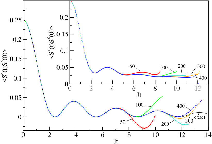
Figure 8: Autocorrelation function for $\Delta=0$ and $\Delta=1$ (inset) at $T=\infty$ where $N=50-400$ states have been kept and $\delta=0.1$. The exact result is shown for comparison in the case $\Delta=0$.

For $\Delta=0$ the $XXZ$-model corresponds to free spinless fermions and is exactly solvable. We focus on the case of free fermions, as here the analysis of the dynamical TMRG (DTMRG) method, its results and numerical errors can be done to much greater extent than in the general case. The performance of the DTMRG itself is expected to be independent of the strength of the interaction. The comparison with the exact result in Fig. 8 shows that the maximum time before the DTMRG algorithm breaks down increases with the number of states. However, the improvement when taking $N=400$ instead of $N=300$ states is marginal. The reason for the breakdown of the DTMRG computation can be traced back to an increase of the discarded weight (see inset of Fig. 9).

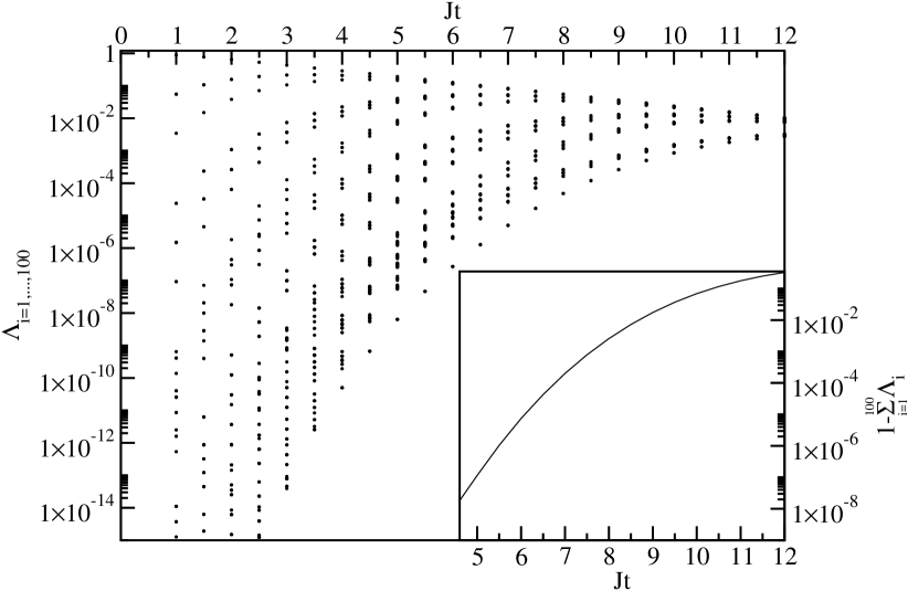
Figure 9: Largest 100 eigenvalues $\Lambda_{i}$ of $\rho_{S}$ for $\Delta=0$ and $T=\infty$ calculated exactly. The inset shows the discarded weight $1-\sum_{i=1}^{100}\Lambda_{i}$.

Throughout the RG procedure we keep only $N$ of the leading eigenstates of the reduced density matrix $\rho_{S}$. As long as the discarded states carry a total weight less than, say, $10^{-3}$ the results are faithful. For infinite temperature and $\Delta=0$ we could explain the rapid increase of the discarded weight with time by deriving an explicit expression for the leading eigenstate of the QTM as well as for the corresponding reduced density matrix. At the free fermion point the spectrum of this density matrix is multiplicative. Hence, from the one-particle spectrum which is calculated by simple numerics we obtain the entire spectrum. As shown in Fig. 9 this spectrum becomes more dense with increasing time thus setting a characteristic time scale $t_{c}(N)$, quite independent of the discretization $\delta$ of the real time, where the algorithm breaks down. Despite these limitations, it is often possible to extrapolate the numerical data to larger times using physical arguments thus allowing to obtain frequency-dependent quantities by a direct Fourier transform. This way the spin-lattice relaxation rate for the Heisenberg chain has been successfully calculated SirkerDiff .

- (1) S.R. White, Phys. Rev. Lett. 69, 2863 (1992)
- (2) T. Nishino, J. Phys. Soc. Jpn. 64, 3598 (1995)
- (3) H.F. Trotter, Proc. Amer. Math. Soc. 10, 545 (1959)
- (4) M. Suzuki, Commun. Math. Phys. 51, 183 (1976)
- (5) M. Suzuki, Phys. Rev. B 31, 2957 (1985)
- (6) R.J. Bursill, T. Xiang, G.A. Gehring, J. Phys. Cond. Mat. 8, L583 (1996)
- (7) X. Wang, T. Xiang, Phys. Rev. B 56, 5061 (1997)
- (8) N. Shibata, J. Phys. Soc. Jpn. 66, 2221 (1997)
- (9) S. Eggert, S. Rommer, Phys. Rev. Lett. 81, 1690 (1998)
- (10) A. Klümper, R. Raupach, F. Schönfeld, Phys. Rev. B 59, 3612 (1999)
- (11) B. Ammon, M. Troyer, T.M. Rice, N. Shibata, Phys. Rev. Lett. 82, 3855 (1999)
- (12) J. Sirker, G. Khaliullin, Phys. Rev. B 67, 100408(R) (2003)
- (13) J. Sirker, Phys. Rev. B 69, 104428 (2004)
- (14) T. Mutou, N. Shibata, K. Ueda, Phys. Rev. Lett. 81, 4939 (1998)
- (15) J. Sirker, A. Klümper, Europhys. Lett. 60, 262 (2002)
- (16) J. Sirker, A. Klümper, Phys. Rev. B 66, 245102 (2002)
- (17) F. Naef, X. Wang, X. Zotos, W. von der Linden, Phys. Rev. B 60, 359 (1999)
- (18) S. Rommer, S. Eggert, Phys. Rev. B 59, 6301 (1999)
- (19) J. Sirker, A. Klümper, Phys. Rev. B 71, 241101(R) (2005)
- (20) I. Peschel, X. Wang, M. Kaulke, K. Hallberg (eds.), Density-Matrix Renormalization, Lecture Notes in Physics, vol. 528 (Springer, Berlin, 1999). And references therein
- (21) J. Sirker, Transfer matrix approach to thermodynamics and dynamics of one-dimensional quantum systems. Ph.D. thesis, Universität Dortmund (2002)
- (22) M. Oshikawa, I. Affleck, Phys. Rev. Lett. 79, 2883 (1997)
- (23) S. Glocke, A. Klümper, H. Rakoto, J.M. Broto, A.U.B. Wolter, S. Süllow, Phys. Rev. B 73, 220403(R) (2006)
- (24) M. Oshikawa, I. Affleck, Phys. Rev. B 60, 1038 (1999)
- (25) S. Eggert, I. Affleck, Phys. Rev. B 46, 10866 (1992)
- (26) S. Fujimoto, S. Eggert, Phys. Rev. Lett. 92, 037206 (2004)
- (27) J. Sirker, M. Bortz, J. Stat. Mech. p. P01007 (2006)
- (28) A. Furusaki, T. Hikihara, Phys. Rev. B 69, 094429 (2004)
- (29) J. Sirker, N. Laflorencie, S. Fujimoto, S. Eggert, I. Affleck, cond-mat/0610165 (2006)
- (30) S. Eggert, I. Affleck, Phys. Rev. Lett. 75, 934 (1995)
- (31) M. Bortz, J. Sirker, J. Phys. A: Math. Gen. 38, 5957 (2005)
- (32) J. Sirker, Phys. Rev. B 73, 224424 (2006)