Mode statistics in random lasers

Abstract

Representing an ensemble of random lasers with an ensemble of random matrices, we compute average number of lasing modes and its fluctuations. The regimes of weak and strong coupling of the passive resonator to environment are considered. In the latter case, contrary to an earlier claim in the literature, we do not find a power-law dependence of the average mode number on the pump strength. For the relative fluctuations, however, a power law can be established. It is shown that, due to the mode competition, the distribution of the number of excited modes over an ensemble of lasers is not binomial.

I Introduction

Random lasers with coherent feedback (see Ref. Cao (2003) for a review) are systems based on active disordered materials where self-sustained radiation modes can be formed. Another possibility involves sufficiently open wave-chaotic resonators filled with active media. In the absence of pumping, both realizations are characterized by short-lived strongly interacting passive modes. In order to treat such systems, the standard laser theory Sargent III et al. (1974); Haken (1985), which assumes an almost closed resonator, needs to be modified. The first step in this direction was made in Ref. Hackenbroich et al. (2002), where the Langevin formalism was adapted to the present situation. The authors described lasing-mode oscillations by non-Hermitian matrices and derived an expression for the linewidth. In Ref. Hackenbroich et al. (2003) a connection was made between the Langevin and the master equations. An improved treatment of non-linearities in the multimode laser theory was proposed in Ref. Türeci et al. .

An interesting problem (also from experimentalist’s standpoint) is the effect of mode competition on the number of lasing modes. Equations yielding this number were derived in Refs. Haken and Sauermann (1963); Misirpashaev and Beenakker (1998) for a weakly open resonator. The authors of Ref. Misirpashaev and Beenakker (1998) discovered that the average number of modes varies (within certain limits) as a power of the pump strength. The theory is based on the fact that the passive-mode widths for a weakly open resonator follow a $\chi^{2}$ distribution. The results were tested numerically by generating ensembles of possible widths according to this distribution. In Ref. Hackenbroich (2005) the mode-number equation of Ref. Misirpashaev and Beenakker (1998) was rederived for a resonator with overlapping passive modes. In particular, Ref. Hackenbroich (2005) exploits a possibility to reproduce statistical properties of modes in open chaotic resonators with the specially chosen ensembles of non-Hermitian random matrices. The average mode number was computed from sets of passive-mode widths obtained directly from these ensembles. It was claimed Hackenbroich (2005) that this number has a power-law dependence on pumping in a resonator strongly coupled to the environment. The theory of Ref. Hackenbroich (2005) relies on the eigenvector and eigenvalue statistics of non-Hermitian random matrices, which was extensively studied in the literature Fyodorov and Sommers (1997); Fyodorov and Khoruzhenko (1999); Sommers et al. (1999); Fyodorov and Sommers (2003). However, general analytical expressions for the relevant correlations of the left and right eigenvectors are still unknown. The correlations were carefully studied numerically in Ref. Hackenbroich (2005).

In the present paper we employ the approach of Ref. Hackenbroich (2005) to study the average number of excited modes and, for the first time, its fluctuations. In the weak-coupling case, our results for the average agree with the predictions of Ref. Misirpashaev and Beenakker (1998). For strong coupling, contrary to the results of Ref. Hackenbroich (2005), we do not find a power law for the average, but do find it for the relative fluctuations. Relating the average number of lasing modes to its fluctuations, it is possible to extract some information about the distribution of this number over an ensemble of lasers. We argue that a binomial distribution gets distorted by the passive-mode overlap and the active-mode competition.

II Theoretical background

We begin by recalling the derivation of Eq. (32) Misirpashaev and Beenakker (1998); Hackenbroich (2005), which yields the number of lasing modes for a given pump strength. This equation is analyzed numerically in the subsequent sections.

II.1 Langevin equations

The system under consideration comprises an open resonator filled with $\mathcal{N}$ identical atoms. A random laser can be modeled by a resonator with an irregular shape, such that its eigenfunctions are chaotic. The system Hamiltonian

$$H_{\text{sys}}=H_{\text{f}}+H_{\text{a}}+H_{\text{f-a}}$$ (1)

is a sum of the radiation-field Hamiltonian $H_{\text{f}}$, atomic Hamiltonian $H_{\text{a}}$, and their interaction $H_{\text{f-a}}$.

It is convenient to represent the system as field and atoms in an ideal (isolated) resonator interacting with environment (heat and pump reservoirs, or baths). The reservoir degrees of freedom are then eliminated. The reservoirs acting on the field and on the atoms are assumed to be independent of each other Haken (1984). Accordingly, the field Hamiltonian can be written in the form

$$H_{\text{f}}=\hbar\sum_{\lambda}\omega_{\lambda}\,a_{\lambda}^{\dagger}a_{\lambda}+\Delta H_{\text{f}},$$ (2)

where $a_{\lambda}$ are the annihilation operators for the modes of the closed resonator with frequencies $\omega_{\lambda}$ and $\Delta H_{\text{f}}$ includes the bath Hamiltonian and the resonator-bath interaction. In the case of an empty resonator with an opening, the role of the reservoir is played by an external field having a continuous spectrum. This model, adopted also for the present paper, was carefully studied in Refs. Viviescas and Hackenbroich (2003, 2004), where, in particular, the ways to split the field into the internal (resonator) and external (bath) parts were discussed.

The atoms will be approximated by their two active levels separated by energy $\hbar\nu$. Given the Fermionic operators $c_{1,2}$ for the levels, one can define the pseudospin-$1/2$ operators $\sigma\equiv s_{x}-is_{y}=c_{1}^{\dagger}c_{2}$ and $s\equiv s_{z}=\frac{1}{2}\left(c_{2}^{\dagger}c_{2}-c_{1}^{\dagger}c_{1}\right)$, i.e., $s_{i}$ generate a spin su(2) algebra. The spin operators $\sigma_{p}$ and $s_{p}$ ($p=1,\ldots,\mathcal{N}$) of different atoms commute. The atomic Hamiltonian becomes

$$H_{\text{a}}=\hbar\nu\sum_{p=1}^{\mathcal{N}}s_{p}+\Delta H_{\text{a}},$$ (3)

where the reservoir operators are contained in $\Delta H_{\text{a}}$.

The interaction Hamiltonian

$$H_{\text{f-a}}=i\hbar\sum_{\lambda p}\left(g_{\lambda p}a_{\lambda}^{\dagger}\sigma_{p}-\text{h.c.}\right)$$ (4)

is written in the rotating-wave and dipole approximations. The former neglects the terms proportional to $a_{\lambda}\sigma_{p}$ and $a_{\lambda}^{\dagger}\sigma_{p}^{\dagger}$. Since $\nu\sim\omega_{\lambda}$, such antiresonant products would oscillate with a double optical frequency in the interaction picture. The latter approximation can be applied since the optical wavelength is much larger than the atom size. Then the coupling constant (in the Gaussian units)

$$g_{\lambda p}=\nu\,\sqrt{\frac{2\pi}{\hbar\omega_{\lambda}}}\,\mathbf{d}_{21}\cdot\boldsymbol{\phi}_{\lambda}^{*}(\mathbf{r}_{p})$$ (5)

is expressed in terms of the dipole moment $\mathbf{d}_{21}$ for the $1\to 2$ transition between the atomic levels, as well as the normalized vector-valued eigenfunction $\boldsymbol{\phi}_{\lambda}(\mathbf{r}_{p})$ of the mode $\lambda$ at the atom position $\mathbf{r}_{p}$ Walls and Milburn (1995). In chaotic resonators the values of an eigenfunction at any two positions are uncorrelated (apart from normalization and boundary effects) if they are more than a wavelength apart Berry (1977). Hence, the couplings $g_{\lambda p}$ can be treated as independent Gaussian random variables.

In the Heisenberg picture, an equation of motion for an operator $O$ is $\dot{O}=\frac{i}{\hbar}\left[H,O\right]$. For the laser operators $a_{\lambda}$, $\sigma_{p}$, and $s_{p}$, the equations of motion can be cast in the form of Langevin equations:

$$\dot{a}_{\lambda}=-i\omega_{\lambda}a_{\lambda}-\sum_{\lambda^{\prime}}\gamma_{\lambda\lambda^{\prime}}a_{\lambda^{\prime}}+\sum_{p^{\prime}}g_{\lambda p^{\prime}}\sigma_{p^{\prime}}+F_{\lambda},$$ (6)

$$\dot{\sigma}_{p}=-\left(i\nu+\gamma_{\perp}\right)\sigma_{p}+2\sum_{\lambda^{\prime}}g_{\lambda^{\prime}p}^{*}\,a_{\lambda^{\prime}}s_{p}+F^{\sigma}_{p},$$ (7)

$$\dot{s}_{p}=\gamma_{\parallel}\left(S-s_{p}\right)-\sum_{\lambda^{\prime}}\left(g_{\lambda^{\prime}p}\,a_{\lambda^{\prime}}^{\dagger}\,\sigma_{p}+\text{h.c.}\right)+F^{s}_{p}.$$ (8)

The reservoirs enter the equations via the damping ($\gamma_{\lambda\lambda^{\prime}}$, $\gamma_{\perp}$, $\gamma_{\parallel}$) and pumping ($S$) parameters and the operators of stochastic forces ($F_{\lambda}$, $F^{\sigma}_{p}$, $F^{s}_{p}$). The latter have zero reservoir average and are $\delta$-correlated in time. This property is a consequence of the Markov approximation, which requires the reservoir relaxation time to be much smaller than all the other time scales. Equations (6)-(8) are appropriate for chaotic resonators. They differ from the standard equations of the laser theory Haken (1985) in to aspects: the non-diagonality of $\gamma_{\lambda\lambda^{\prime}}$ and the randomness of $g_{\lambda p}$. Equation (6) was derived in Refs. Viviescas and Hackenbroich (2003); Hackenbroich et al. (2003). The damping matrix $\gamma_{\lambda\lambda^{\prime}}$ is Hermitian. It is strongly non-diagonal if the resonator modes are overlapping. The off-diagonal elements point to the interaction between the respective modes via a coupling to the continuum. Equations (7) and (8) follow, e.g., from the Langevin theory for three-level atoms Sargent III et al. (1974) if the total population of the two active levels is kept constant. $\gamma_{\perp}$ and $\gamma_{\parallel}$ are the polarization and inversion decay constants, respectively.

In the following, we work in the classical approximation, whereby the noise forces are neglected and the operators are treated as c-numbers (the prior notation will be retained). This approximation fails near the lasing threshold, where the average intensity is smaller than its quantum fluctuations. The classical version of Eqs. (6)-(8) becomes

$$\frac{d}{dt}|a\rangle=-i\hat{\Omega}|a\rangle+\sum_{p^{\prime}}|g_{p^{\prime}}\rangle\,\sigma_{p^{\prime}},$$ (9)

$$\dot{\sigma}_{p}=-\left(i\nu+\gamma_{\perp}\right)\sigma_{p}+2\,\langle g_{p}|a\rangle\,s_{p},$$ (10)

$$\dot{s}_{p}=\gamma_{\parallel}\left(S-s_{p}\right)-\left(\langle a|g_{p}\rangle\,\sigma_{p}+\text{c.c.}\right).$$ (11)

Here, for the compactness of notation, we introduced the classical vectors $|a\rangle=(\ldots,a_{\lambda},a_{\lambda+1},\ldots)^{T}$ and $|g_{p}\rangle\ =(\ldots,g_{\lambda p},g_{\lambda+1,p},\ldots)^{T}$ and the matrix

$$\bigl{(}\hat{\Omega}\bigr{)}_{\lambda\lambda^{\prime}}=\omega_{\lambda}\delta_{\lambda\lambda^{\prime}}-i\gamma_{\lambda\lambda^{\prime}}.$$ (12)

Since $\hat{\Omega}$ is not Hermitian, it has different left and right eigenbases $\langle L_{k}|$ and $|R_{k}\rangle$, respectively. Thus, its spectral decomposition is of the form

$$\hat{\Omega}=\sum_{k}|R_{k}\rangle\left(\Omega_{k}-i\kappa_{k}\right)\langle L_{k}|,$$ (13)

where the eigenvectors are normalized in such a way that $\langle L_{k}|R_{k^{\prime}}\rangle=\delta_{kk^{\prime}}$ and $\langle R_{k}|R_{k}\rangle=1$, but, in general, $\langle R_{k}|R_{k^{\prime}}\rangle\neq\delta_{kk^{\prime}}$. $\Omega_{k}-i\kappa_{k}$ ($\kappa_{k}>0$) are the complex eigenfrequencies of the passive open resonator. We expand $|a\rangle=\sum_{k}\alpha_{k}|R_{k}\rangle$, where the amplitudes

$$\alpha_{k}=\langle L_{k}|a\rangle,$$ (14)

satisfy the equations

$$\dot{\alpha}_{k}=-\left(i\Omega_{k}+\kappa_{k}\right)\alpha_{k}+\sum_{p^{\prime}}\langle L_{k}|g_{p^{\prime}}\rangle\,\sigma_{p^{\prime}},$$ (15)

$$\dot{\sigma}_{p}=-\left(i\nu+\gamma_{\perp}\right)\sigma_{p}+2\sum_{k^{\prime}}\langle g_{p}|R_{k^{\prime}}\rangle\,\alpha_{k^{\prime}}s_{p},$$ (16)

$$\dot{s}_{p}=\gamma_{\parallel}\left(S-s_{p}\right)-\sum_{k^{\prime}}\left(\langle R_{k^{\prime}}|g_{p}\rangle\,\alpha_{k^{\prime}}^{*}\sigma_{p}+\text{c.c.}\right)$$ (17)

following from Eqs. (9)-(11). It is worth emphasizing again that the open-resonator modes $k$ are coupled through the interaction with the atoms, while the closed-resonator modes $\lambda$, in addition, interact via the reservoir.

II.2 Number of lasing modes

We solve Eqs. (15)-(17) by treating the interaction with the atoms perturbatively. Namely, it will be assumed that the sustained field oscillations are proportional to the unperturbed eigenvectors $|R_{k}\rangle$. However, the oscillation frequencies $\overline{\Omega}_{k}\approx\Omega_{k}$ are to be determined selfconsistently. It was argued in Ref. Fu and Haken (1991), that a multimode solution is possible if

$$\kappa_{k},\gamma_{\parallel}\ll\Delta\overline{\Omega},\gamma_{\perp},$$ (18)

where $\Delta\overline{\Omega}$ is a typical spacing between the lasing-mode frequencies. This condition ensures that the population inversion $s_{p}$ is approximately constant in time . An expression for $s_{p}$ can be derived as follows. First, one represents the polarization $\sigma_{p}=\sum_{k}\sigma_{pk}$ as a sum of single-frequency components $\sigma_{pk}\propto\exp\left(-i\overline{\Omega}_{k}t\right)$. Using Eq. (16) with $s_{p}=\text{const}$,

$$\sigma_{pk}=\frac{2s_{p}\langle g_{p}|R_{k}\rangle}{-i\left(\overline{\Omega}_{k}-\nu\right)+\gamma_{\perp}}\,\alpha_{k}$$ (19)

is expressed in terms of $\alpha_{k}$, which oscillates with the same frequency. Finally, these $\sigma_{pk}$ are substituted to Eq. (17) yielding

$$s_{p}\approx\frac{S}{Y_{p}},$$ (20)

$$Y_{p}\equiv 1+\frac{4}{\gamma_{\perp}\gamma_{\parallel}}\sum_{k}|\langle g_{p}|R_{k}\rangle|^{2}\mathcal{L}_{k}\,|\alpha_{k}|^{2},$$ (21)

$$\mathcal{L}_{k}\equiv\left[1+\left(\overline{\Omega}_{k}-\nu\right)^{2}/\gamma_{\perp}^{2}\right]^{-1},$$ (22)

where the oscillating products $\alpha_{k}^{*}\alpha_{k^{\prime}}$, $k\neq k^{\prime}$, were averaged out, in line with the constant-$s_{p}$ approximation. Taking into account Eqs. (19) and (20) and keeping only the terms oscillating with frequency $\overline{\Omega}_{k}$ in Eq. (15), we arrive at an equation for $\alpha_{k}$,

$$\dot{\alpha}_{k}\approx-\left(i\Omega_{k}+\kappa_{k}-B_{k}\right)\alpha_{k},$$ (23)

$$B_{k}\equiv\frac{2S}{-i\left(\overline{\Omega}_{k}-\nu\right)+\gamma_{\perp}}\,\langle L_{k}|\sum_{p}\frac{|g_{p}\rangle\langle g_{p}|}{Y_{p}}|R_{k}\rangle.$$ (24)

Equations (23) for $N$ lasing modes are equivalent to a system of $2N$ real equations Hackenbroich (2005),

$$\overline{\Omega}_{k}=\Omega_{k}-\text{Im}\,B_{k},$$ (25)

$$\text{Re}\,B_{k}=\kappa_{k},$$ (26)

from which the frequencies $\overline{\Omega}_{k}$ and the intensities $I_{k}=|\alpha_{k}|^{2}$ of the lasing modes can be determined. Equations (25) and (26) are valid only for such $k$ that $I_{k}>0$.

Further progress can be made if $Y_{p}^{-1}$ in Eq. (24) is expanded up to the linear terms in $I_{k}$. This procedure presumes that the laser is operating not far from the threshold. When the atoms are distributed uniformly over the resonator and their density is sufficiently large, the $p$ sum becomes a volume integral. Then the summations entering Eq. (24) are computed as follows:

$$\sum_{p}|g_{p}\rangle\langle g_{p}|\to\mathcal{N}g^{2}\int d^{3}r\,|\phi^{*}(\mathbf{r})\rangle\langle\phi^{*}(\mathbf{r})|=\mathcal{N}g^{2},$$ (27)

$$\sum_{p}\langle L_{k}|g_{p}\rangle\langle g_{p}|R_{k}\rangle|\langle g_{p}|R_{k^{\prime}}\rangle|^{2}$$

$$\to\mathcal{N}g^{4}V\int d^{3}r\,\langle L_{k}|\phi^{*}(\mathbf{r})\rangle\langle\phi^{*}(\mathbf{r})|R_{k}\rangle|\langle\phi^{*}(\mathbf{r})|R_{k^{\prime}}\rangle|^{2}$$

$$\approx\mathcal{N}g^{4}(1+2\delta_{kk^{\prime}}).$$ (28)

where $|\phi(\mathbf{r})\rangle=\bigl{(}\ldots,\phi_{\lambda}(\mathbf{r}),\phi_{\lambda+1}(\mathbf{r}),\ldots\bigr{)}^{T}$,

$$g=\sqrt{\frac{2\pi\nu}{\hbar V}}\,|\mathbf{d}_{21}|,$$ (29)

and $V$ is the resonator volume. Above we assumed that all the modes $\lambda$ are polarized along $\mathbf{d}_{21}$ and $\omega_{\lambda}\approx\nu$. The approximate equality in Eq. (28) results from treating the wavefunctions $\langle L_{k}|\phi^{*}(\mathbf{r})\rangle$ and $\langle\phi^{*}(\mathbf{r})|R_{k}\rangle$ in a wave-chaotic resonator as Gaussian random variables, restricted only by normalization. Performing random-matrix simulations, this property was shown to hold in the relevant range of the mode widths Hackenbroich (2005). Using Eqs. (27) and (28), we arrive at

$$B_{k}= \frac{2S\mathcal{N}g^{2}}{\gamma_{\perp}}\mathcal{L}_{k}\left(1+i\frac{\overline{\Omega}_{k}-\nu}{\gamma_{\perp}}\right)$$

$$\times\left[1-\frac{4g^{2}}{\gamma_{\perp}\gamma_{\parallel}}\sum_{k^{\prime}}I_{k^{\prime}}\mathcal{L}_{k^{\prime}}(1+2\delta_{kk^{\prime}})\right]+O(I^{2}).$$ (30)

The linear gain $G_{0}\mathcal{L}_{k}$, where

$$G_{0}\equiv\frac{2\mathcal{N}g^{2}}{\gamma_{\perp}}\,S,$$ (31)

is obtained from $\text{Re}\,B_{k}$ by setting $I_{k^{\prime}}=0$.

To determine the number of lasing modes, we approximate $\overline{\Omega}_{k}$ with $\Omega_{k}$, substitute $B_{k}$ (30) in Eq. (26), divide it by $\mathcal{L}_{k}$, sum over $k$, and find $\sum_{k^{\prime}}I_{k^{\prime}}\mathcal{L}_{k^{\prime}}$. Then $\sum_{k^{\prime}}I_{k^{\prime}}\mathcal{L}_{k^{\prime}}$ can be used in Eq. (26) to express $I_{k}$, which is required to be positive for all lasing modes. This condition yields Misirpashaev and Beenakker (1998)

$$\frac{\kappa_{N}}{\mathcal{L}_{N}}+\frac{1}{2}\left(N\frac{\kappa_{N}}{\mathcal{L}_{N}}-\sum_{k=1}^{N}\frac{\kappa_{k}}{\mathcal{L}_{k}}\right)<G_{0},$$ (32)

where the modes are ordered in such a way that $\kappa_{1}/\mathcal{L}_{1}\leq\kappa_{2}/\mathcal{L}_{2}\leq\ldots$. The largest $N$ satisfying this inequality is the number of lasing modes. On the other hand, the largest $N_{0}$ such that

$$\frac{\kappa_{N_{0}}}{\mathcal{L}_{N_{0}}}<G_{0}$$ (33)

holds, is the number of modes that would lase in the absence of mode competition. These are the modes for which the linear gain exceeds the losses. Clearly, ${N_{0}\geq N}$.

III Average number of lasing modes and its fluctuations

III.1 Random-matrix model

We investigated the mode statistics resulting from Eqs. (32) and (33). Ensembles of open chaotic resonators were modeled by randomly generated non-Hermitian matrices $\hat{\Omega}\equiv\hat{\omega}-i\hat{\gamma}$ (12). In the basis of the modes $\lambda$, $\hat{\Omega}$ has a diagonal real part. Its imaginary part is of the form Hackenbroich et al. (2003)

$$-\hat{\gamma}=-\pi\hat{W}\hat{W}^{\dagger},$$ (34)

where $\bigl{(}\hat{W}\bigr{)}_{\lambda m}$ ($\lambda=1,\ldots,L$, $m=1,\ldots,M\leq L$) describes interaction of the resonator mode $\lambda$ with the $m$th channel of the reservoir. Each channel includes a continuum of frequencies. However, $\hat{W}$ is frequency independent in the Markov approximation. Clearly, the matrix $\hat{\gamma}$ has at most $M$ nonzero eigenvalues $\gamma_{i}$, $i=1,\ldots,M$ (it is possible to find $N-M$ linearly independent vectors orthogonal to the rows of $\hat{W}^{\dagger}$). We will consider the case of equivalent channels, when all $\gamma_{i}=\gamma$.

A matrix $\hat{\Omega}$ is most easily constructed in the basis where $\hat{\gamma}$ is diagonal: we fix $\hat{\gamma}$ and choose $\hat{\omega}$ from a Gaussian orthogonal ensemble Sommers et al. (1999). Without loss of generality, the diagonal and off-diagonal elements of $\hat{\omega}$ are taken from a normal distribution with zero mean and the variance of $2/L$ and $1/L$, respectively. In the limit $L\gg 1$, $\Omega_{k}$ (13) (the real parts of the eigenvalues of $\hat{\Omega}$) are distributed according to the Wigner semicircle law

$$\rho(\Omega)=\frac{1}{\pi}\sqrt{1-\frac{\Omega^{2}}{4}},\quad-2\leq\Omega\leq 2,$$ (35)

where $\rho(\Omega)$ is normalized to unity. Numerical simulations (Fig. 1) show a reasonable agreement with this equation. The strength of coupling to continuum is characterized by a parameter $2\pi\rho(\Omega)/\left(\gamma+\gamma^{-1}\right)$ Sommers et al. (1999). Thus, it is sufficient to consider $\gamma\in[0,1]$, whereby $\gamma=0$ ($\gamma=1$) corresponds to the vanishing (strongest) coupling. Importantly, even within one matrix $\hat{\Omega}$, the effective coupling depends on the spectral region according to $\rho(\Omega)$.

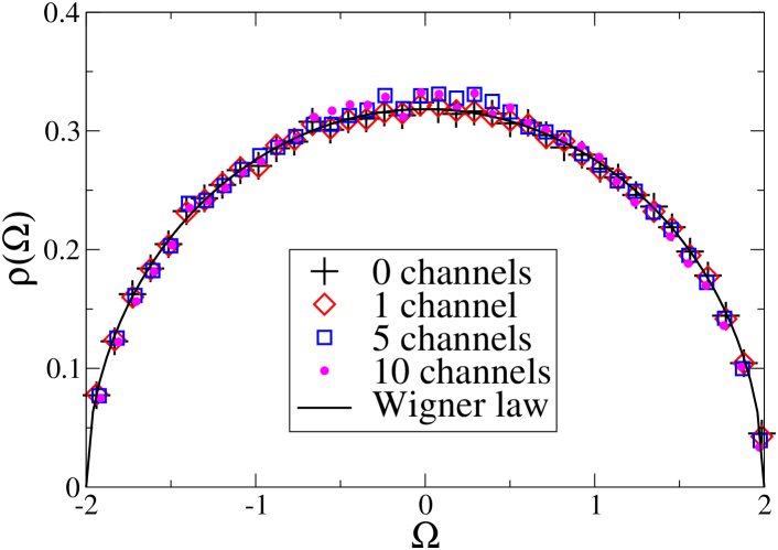
Figure 1: (Color online) Distribution $\rho(\Omega)$ of the real parts of the eigenvalues of random matrices. Numerical simulations were performed for an ensemble of 500 matrices of size $L=200$ coupled to $M=0$, $1$, $5$, and $10$ open channels with the coupling $\gamma=1$. Analytical expression (35) is plotted for comparison.

III.2 Results and discussion

In the following figures, we present results of numerical simulations for the average number of lasing modes $\langle N\rangle$ and its standard deviation $\sigma_{N}$. The respective quantities in the absence of the mode competition, $\langle N_{0}\rangle$ and $\sigma_{N_{0}}$, were calculated as well. The averages were performed over ensembles of random matrices. As was explained earlier, the effective coupling to continuum depends on $\rho(\Omega)$. Therefore, for each matrix, of all eigenvalues, only $L_{0}\approx 0.36L$ eigenvalues closest to the top of the Wigner semicircle were used in Eqs. (32) and (33). Within this spectral region, $\rho(\Omega)$ varies by about 4%. In order to reduce the number of parameters, we assumed that $\gamma_{\perp}$ is sufficiently large, and set $\mathcal{L}_{k}=1$. The pumping was measured in units of its threshold value $S_{\text{thr}}$, which was determined numerically from the threshold condition $\langle N\rangle=1$. An estimate yields $S/S_{\text{thr}}\sim G_{0}/\kappa_{0}$, where $\kappa_{0}\sim\gamma M/L$ is a typical loss.

First, we discuss a weakly open resonator, $\kappa_{0}\ll\Delta\Omega\approx\pi/L$, where $\Delta\Omega$ is the mean nearest-neighbor spacing between $\Omega_{k}$. A theory for the averages $\langle N\rangle$ and $\langle N_{0}\rangle$ in this regime was proposed in Ref. Misirpashaev and Beenakker (1998). Central to the argument is the analytical expression for the distribution of $\kappa_{k}$ (13),

$$P(y)=\frac{(M/2)^{M/2}}{\Gamma(M/2)}\,y^{\frac{M}{2}-1}\exp\left(-\frac{M}{2}\,y\right),\quad y\equiv\kappa/\overline{\kappa},$$ (36)

where $\overline{\kappa}$ is the average of $\kappa$ and $\Gamma(z)$ is the gamma function Abramowitz and Stegun (1972). $P(y)$ is a $\chi^{2}$ distribution with $M$ degrees of freedom and the average $\overline{y}=1$. The average number of modes in the absence of competition can be estimated from

$$\langle N_{0}\rangle=L_{0}\int_{0}^{G_{0}/\overline{\kappa}}dy\,P(y)=L_{0}\,\frac{\gamma\left(\frac{M}{2},\frac{M}{2}\frac{G_{0}}{\overline{\kappa}}\right)}{\Gamma(M/2)},$$ (37)

where $\gamma(z,x)=\int_{0}^{x}dt\,t^{z-1}e^{-t}$ is the incomplete gamma function Abramowitz and Stegun (1972). The numerical results in Fig. 2 show a good agreement with this prediction. In the weak-pump regime $G_{0}/\overline{\kappa}\ll 1$, there is a power law $\langle N_{0}\rangle\propto S^{M/2}$ Misirpashaev and Beenakker (1998). With the increased pumping, the saturation $\langle N_{0}\rangle\to L_{0}$ sets in. Clearly, this form of saturation is an artifact of our model. Normally, the number of potential lasing modes would be limited by the Lorentzians $\mathcal{L}_{k}$. Nevertheless, for large $L_{0}$, the present model is appropriate below the saturation.

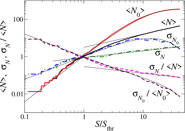
Figure 2: (Color online) Average number of lasing modes $\langle N\rangle$, its standard deviation $\sigma_{N}$, and relative standard deviation $\sigma_{N}/\langle N\rangle$, as a function of pumping. The same in the absence of mode competition ($\langle N_{0}\rangle$, $\sigma_{N_{0}}$, $\sigma_{N_{0}}/\langle N_{0}\rangle$). The thin solid lines display analytical results of Eqs. (37) and (38) and power-law asymptotics. Numerical simulations were performed for an ensemble of 75 random matrices of size $L=1000$ coupled to $M=5$ open channels with the coupling $\gamma=0.1$. $L_{0}=360$ eigenvalues per matrix were taken into account. The analytical functions were computed with the parameters $\overline{\kappa}=5.0\times 10^{-4}$ and $G_{0}\left|{}_{S=S_{\text{thr}}}\right.=3.3\times 10^{-5}$, which were extracted from the ensemble.

In order to determine $\sigma_{N_{0}}$, it is the simplest to assume that $N_{0}=1,\ldots,L_{0}$ is distributed according to a binomial distribution $P_{p}(N_{0}|L_{0})$, where $p=\langle N_{0}\rangle/L_{0}$ is the probability for a given mode to lase. The standard deviation for this distribution is known to be

$$\sigma_{N_{0}}=\sqrt{\langle N_{0}\rangle\left(1-\frac{\langle N_{0}\rangle}{L_{0}}\right)},$$ (38)

where $\langle N_{0}\rangle$ can be substituted from Eq. (37). A comparison with the numerical curve in Fig. 2 supports our assumption. When $\langle N_{0}\rangle\ll L_{0}$, we find a power law $\sigma_{N_{0}}\propto\sqrt{\langle N_{0}\rangle}\propto S^{M/4}$.

In the presence of mode competition, it is interesting to look at the case when $\langle N\rangle$ is far below the saturation, but, still, sufficiently large. The former condition yields $\langle N\rangle\propto\kappa^{M/2}$, while the latter ensures that the terms of order $N\kappa_{N}\approx\langle N\rangle\kappa$ dominate the left-hand side of Eq. (32). Combination of the two estimates gives $\langle N\rangle\propto S^{\frac{M}{M+2}}$ Misirpashaev and Beenakker (1998). We checked numerically (via $\sigma_{N}$) that the $N$ distribution is not binomial. Nevertheless, the power law $\sigma_{N}\propto\sqrt{\langle N\rangle}\propto S^{\frac{M}{2(M+2)}}$ remains valid (Fig. 2).

Next, we consider the problem of a strong coupling to the bath ($\kappa_{0}\sim\Delta\Omega$) modeled here by a random-matrix ensemble with $\gamma=1$. The distribution $P(y)$ in this case is no longer given by Eq. (36), but rather has a power-law tail $P(y)\propto y^{-2}$, $y\gg 1$ Sommers et al. (1999); its full analytical expression is very complicated. Numerical results for the average number of lasing modes and its fluctuations were obtained for $M=1$, $3$, $5$, $7$, and $10$. The data for $M=5$ are presented in Fig. 3. The $S$ dependencies of $\langle N\rangle$ and $\langle N_{0}\rangle$ here are similar to those found in Ref. Hackenbroich (2005). However, except for $M=1$, we can confirm for these quantities neither a power-law behavior, in general, nor the powers $1/3$, respectively, $1/2$, in particular.

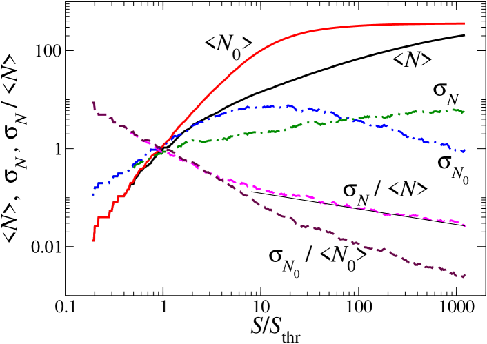
Figure 3: (Color online) Same as in Fig. 2, but with the coupling $\gamma=1.0$. The thin solid line displays a power law with the exponent $-0.32$. The ensemble is characterized by $\overline{\kappa}=7.4\times 10^{-3}$ and $G_{0}\left|{}_{S=S_{\text{thr}}}\right.=1.1\times 10^{-4}$.

An analysis of fluctuations shows that the distributions of $N$ and $N_{0}$ are non-binomial. While the standard deviation $\sigma_{N}$ saturates at large $S$, the relative deviation $\sigma_{N}/\langle N\rangle$ exhibits a power law with the exponent $0.2\div 0.4$, depending on $M$. Examining the numerical data, we discovered an interesting relation between the relative fluctuations of $N_{0}$ and the average of $N$:

$$\frac{\sigma_{N_{0}}}{\langle N_{0}\rangle}\approx\frac{1}{\langle N\rangle}-\frac{1}{L_{0}},\quad\frac{S}{S_{\text{thr}}}\gg 1.$$ (39)

As demonstrated in Fig. 4, this property is well satisfied for $M\neq 1$. Unfortunately, an explanation of this result is still lacking.

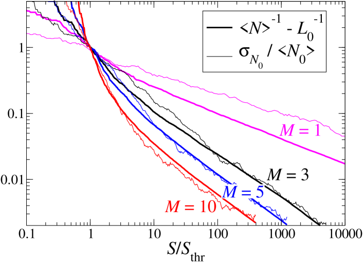
Figure 4: (Color online) Comparison of $\langle N\rangle^{-1}-L_{0}^{-1}$ (thick lines) and $\sigma_{N_{0}}/\langle N_{0}\rangle$ (thin lines) plotted as functions of pumping. The ensembles of random matrices as in Fig. 2, but with the coupling $\gamma=1.0$ and with the number of open channels $M$ labeled in the figure.

IV Conclusions

By modeling ensembles of open chaotic resonators with ensembles of random matrices, we studied average number of lasing modes and its fluctuations. To highlight the effect of mode competition and allow for a better comparison with earlier work, the linear approximation to the lasing equations was considered as well.

In the case of a weakly open resonator, the average number of modes is proportional to a power of pump strength (within a certain pumping range). This result agrees with the analytical prediction in Ref. Misirpashaev and Beenakker (1998). The standard deviation changes as a square root of the average. In the absence of mode competition, the number of modes follows a binomial distribution, if the total number of eigenstates available for lasing is finite. The distribution becomes non-binomial in the presence of mode competition.

For a resonator strongly coupled to the environment, we could not establish any power-law dependence of the average mode number on pumping. (The case of one open channel makes an exception.) This evidence stays in contradiction to the conclusions of Ref. Hackenbroich (2005). On the other hand, we find a power-law behavior for the relative fluctuations. A curious relation (39) between the average with and the relative fluctuation without the mode competition requires further investigation.

As a possible extension of this work, it would be interesting to relax some of the assumptions made. For example, one can consider an effect of the Lorentzian line shape (here approximated as rectangular). A more challenging task is to avoid the near-threshold expansion of the intensity-dependent denominators in Eq. (24).