Modified Kuramoto-Sivashinsky equation: stability of stationary solutions and the consequent dynamics

Abstract

We study the effect of a higher-order nonlinearity in the standard Kuramoto-Sivashinsky equation: $\partial_{x}\tilde{G}(H_{x})$. We find that the stability of steady states depends on $dv/dq$, the derivative of the interface velocity on the wavevector $q$ of the steady state. If the standard nonlinearity vanishes, coarsening is possible, in principle, only if $\tilde{G}$ is an odd function of $H_{x}$. In this case, the equation falls in the category of the generalized Cahn-Hilliard equation, whose dynamical behavior was recently studied by the same authors. Instead, if $\tilde{G}$ is an even function of $H_{x}$, we show that steady-state solutions are not permissible.

I Introduction

One of the most prominent and generic equations that arises in nonequilibrium systems is the Kuramoto-Sivashinsky (KS)Nepo ; KS ; Sivashinsky equation:

$$H_{t}+H_{xxxx}+H_{xx}+HH_{x}=0,$$ (1)

where $H$ is some scalar function (like the slope of a one-dimensional growing front), and differentiations are subscripted. The linear stability analysis of the KS equation (by looking for solutions in the form of $e^{iqx+\omega t}$) yields $\omega=q^{2}-q^{4}$. The (linearly) fastest growing mode has a wavenumber given by $q_{u}=1/\sqrt{2}$ (obtained from $\partial_{q}\omega=0$). For a large box size the KS equation is known to exhibit spatiotemporal chaos. The chaotic pattern statistically selects a length scale which is close to $2\pi/q_{u}$: in fact, the structure factor $\langle|H_{q}|^{2}\rangle$, where $\langle\cdots\rangle$ designates the average over many runs and $H_{q}$ is the Fourier transform of $H$, exhibits a maximum around $q=q_{u}$. Other nonequlibrium equations are known, however, to exhibit different dynamical behaviors: just to limit to one-dimensional systems, we may have coarsening, a diverging amplitude with a fixed wavelength, a frozen pattern, travelling waves, and so on.

An important issue is the recognition of general criteria that enable to predict whether or not coarsening takes place within a class of nonlinear equations, without having to resort to a forward time dependent calculation. In recent works Politi1 ; Politi2 ; CKS we have considered several classes of one-dimensional Partial Differential Equations (PDE), having the form $H_{t}={\cal N}[H]$, where ${\cal N}$ is a nonlinear operator acting on the spatial variable $x$.

Sometimes, even in the presence of strong nonlinearities, the search for steady states reduces to solving a Newton-type equation, $\tilde{H}_{xx}+V(\tilde{H})=0$, where $\tilde{H}$ is some function of $H$. In these cases, $\lambda(A)$, giving the dependence of the wavelength $\lambda$ of the steady state on its amplitude $A$, is a one-value function (see Fig. 1, full lines), and the criterion for the existence of coarsening is expressed in terms of the derivative $\lambda^{\prime}(A)$.

It has been shown that $\lambda^{\prime}(A)$ has minus the sign of the phase diffusion equation. Thus $\lambda^{\prime}(A)>0$ corresponds to a branch which is unstable with respect to the phase of the pattern, entailing thus coarsening. The situation is more complicated when $\lambda(A)$ exhibits a fold (see Fig. 1, dashed line). This event occurs, e.g., in the KS equation and in the Swift-Hohenberg equation. As for the KS equation, which is the topic of this paper, Nepomnyashchii Nepo has shown that the forearm part of the curve $\lambda(A)$ with positive slope, $\lambda^{\prime}(A)>0$, is an unstable branch. This result holds only for the pure KS equation, however.

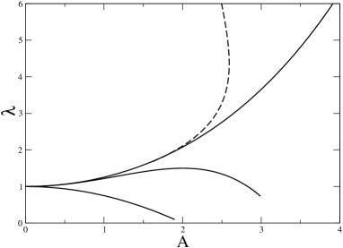
Figure 1: The periodic stationary solutions of some classes of nonlinear equations satisfy a Newton-type equation, $\tilde{H}_{xx}+V(\tilde{H})=0$, and the resulting $\lambda(A)$ is a single-value function. According to the explicit form of $V(\tilde{H})$, we may have the different curves shown as full lines. The dashed line, which displays a fold, corresponds to a non single-value function. It comes out in the Kuramoto-Sivashinsky and in the Swift-Hohenberg equations. Units on both axes are arbitrary.

The aim of this paper is the following. (i) Firstly we shall extend the result of Nepomnyashchii Nepo to a generalized form of the KS equation, which includes higher order nonlinearities. As a way of example, the next leading term in the KS equation ($H_{x}H_{xx}$) has been analyzed in Ihle , and it has been shown that this term significantly affect dynamics; for example the profile may exhibit deep grooves. We shall consider a more general form of the modified KS equation by adding a term like $\partial_{x}\tilde{G}(H_{x})$ (this includes as a particular case the term $H_{x}H_{xx}$). We find that the stability of the steady state solutions depends on $v^{\prime}(q)$, where $v$ is the average interface velocity. (ii) If the standard KS nonlinearity vanishes (no $HH_{x}$ term), then there is coarsening if $\tilde{G}$ is an odd function. In this case a mapping of the equation onto a generalized Cahn-Hilliard equation is straightforward. (iii) If $\tilde{G}$ is even (still in the absence of the standard nonlinearity), we show that there exists no steady-state periodic solution, as attested by numerical simulations for $\tilde{G}=H_{x}^{2}$ CMV .

II The modified KS equation

II.1 The method

We study the following equation:

$$H_{t}+c_{4}H_{xxxx}+c_{2}H_{xx}+\alpha HH_{x}+\beta\partial_{x}\tilde{G}(H_{x})=0,$$ (2)

which reduces to the standard Kuramoto-Sivashinsky equation when $\tilde{G}=0$. A rescaling of $x,t$ and $H$ always allows one to reduce the equation to a one parameter equation, which can be absorbed into a redifinition of $\tilde{G}$. However, for the sake of clarity, we do not get rid of $\alpha$, so that we write

$$H_{t}+H_{xxxx}+H_{xx}+\alpha HH_{x}+\partial_{x}\tilde{G}(H_{x})=0.$$ (3)

It is also useful to rewrite Eq. (3) using the variable $u$, with $u_{x}=H$:

$$u_{t}+u_{xxxx}+u_{xx}+\hbox{${\alpha\over 2}$}u_{x}^{2}+\tilde{G}(u_{xx})=0,$$ (4)

where the integration constant $v_{0}$ can be canceled out by the transformation $u(x,t)\to u(x,t)-v_{0}t$.

Within the $H-$formulation, the average velocity $d\langle H\rangle/dt$ vanishes, because Eq. (3) has the conserved form $H_{t}=-\partial_{x}(\dots)$. Within the $u-$formulation,

$${d\langle u\rangle\over dt}=-\left[{\alpha\over 2}\langle u_{x}^{2}\rangle+\langle\tilde{G}(u_{xx})\rangle\right]=v.$$ (5)

We start from a stationary solution of period $q$, $H(x)$, and perturb it with adding $h(x)\exp(-\omega t)$. The function $h(x)$ therefore satisfies the linear equation

$$h_{xxxx}+h_{xx}+\alpha(hH)_{x}+(h_{x}G(H_{x}))_{x}=\omega h,$$ (6)

where $G=\tilde{G}^{\prime}$ and whose coefficients are periodic with period $\lambda=2\pi/q$. According to the Floquet-Bloch theorem, the solution has the form $h(x)=\exp(iKx)F(x)$, where $F(x)$ has the same period as $H(x)$.

We are interested in weak modulations of long wavelength, i.e. with $K\ll q$. It is therefore convenient to introduce the reduced wavevector $Q=K/q$ and the phase $\phi=qx$. The equation determining the steady state $H(\phi)$ is

$$q^{4}H_{\phi\phi\phi\phi}+q^{2}H_{\phi\phi}+\alpha qHH_{\phi}+q^{2}H_{\phi\phi}G(qH_{\phi})=0$$ (7)

and Eq. (6) reads

$$q^{4}h_{\phi\phi\phi\phi}+q^{2}h_{\phi\phi}+q\alpha(hH)_{\phi}+q^{2}(h_{\phi}G(qH_{\phi}))_{\phi}$$

$$\equiv{\cal L}h=\omega h,$$ (8)

with $h=\exp(iQ\phi)F(\phi)$.

The final step is to expand both $\omega$ and $F(\phi)$ in powers of $Q$,

$$F(\phi) = F_{0}(\phi)+QF_{1}(\phi)+Q^{2}F_{2}(\phi)+\dots$$ (9)

$$\omega = \omega_{0}+Q\omega_{1}+Q^{2}\omega_{2}+\dots$$ (10)

and to solve Eq. (8) at the lowest orders in $Q$.

II.2 Zero order

The differential equation determining the steady state $H(x)$ does not depend explicitely on $x$, so that $H(x+x_{0})$ is a solution as well. This symmetry implies that ${\cal L}h=\omega h$ (see Eq. (8)) is solved by $h=H_{\phi}$ and $\omega=0$, as can be easily checked by taking the $\phi$ derivative of Eq. (7). Since the zero order equation is simply

$${\cal L}F_{0}=0,$$ (11)

we obtain $F_{0}=H_{\phi}$.

II.3 First order

The equation for $F_{1}$ reads

$${\cal L}F_{1}=$$ (12)

$$\omega_{1}H^{\prime}-iq[4q^{3}H^{\prime\prime\prime\prime}+2q(1+G)H^{\prime\prime}+(\alpha H+q^{2}H^{\prime\prime}G^{\prime})H^{\prime}],$$

where we have used the shorthands $H^{\prime}=H_{\phi},H^{\prime\prime}=H_{\phi\phi},\dots$ . If we differentiate Eq. (7) with respect to $q$, we get a similar equation,

$${\cal L}H_{q}=-(4q^{3}H^{\prime\prime\prime\prime}+2qH^{\prime\prime}+\alpha HH^{\prime}+3\beta q^{2}H^{\prime}H^{\prime\prime}).$$ (13)

The comparison of Eqs. (12,13) suggests to look for $F_{1}$ under the form $F_{1}=iqH_{q}+c$, where $c$ is a constant. We easily find $c=\omega_{1}/(\alpha q)$, so that

$$F_{1}={\omega_{1}\over\alpha q}+iqH_{q}.$$ (14)

This result shows that in the absence of the standard nonlinearity, $\alpha=0$, $\omega_{1}$ should vanish whatever $\tilde{G}$ is.

We might have started with an even more general Eq. (3), replacing the standard nonlinearity $(\alpha HH_{x})=\partial_{x}(\hbox{${\alpha\over 2}$}H^{2})$ with $\partial_{x}\tilde{P}(H)$. The term $\alpha HH^{\prime}$ in the right hand sides of Eqs. (12) and (13) would be replaced by $P(H)H^{\prime}$, with $P=\tilde{P}^{\prime}$. However, in the general case $P^{\prime}$ is not a constant: therefore, it is not possible to look for a solution $F_{1}=iqH_{q}+c$.

II.4 Second order

The equation for $F_{2}$ has the form

$${\cal L}F_{2}+q^{2}(1+G)(-F_{0}+2iF_{1}^{\prime})+(\alpha qH+q^{3}H^{\prime\prime}G^{\prime})iF_{1}$$

$$=\omega_{2}F_{0}+\omega_{1}F_{1},$$ (15)

or

$${\cal L}F_{2} = \omega_{2}H^{\prime}+iq\omega_{1}H_{q}+q^{2}H^{\prime}+2q^{3}H_{q}^{\prime}-i\omega_{1}H$$ (16)

$$-i(\omega_{1}/\alpha)q^{2}H^{\prime\prime}G^{\prime}(qH^{\prime})$$

$$+\omega_{1}^{2}/(\alpha q)+q^{2}G(qH^{\prime})H^{\prime}+2q^{3}G(qH^{\prime})H^{\prime}_{q}$$

$$+\alpha q^{2}HH_{q}+q^{4}H^{\prime\prime}G^{\prime}(qH^{\prime})H_{q}.$$

Now we take the $2\pi$-average of the previous equation, getting

$${\omega_{1}^{2}\over\alpha q}+q^{2}\langle G(qH^{\prime})H^{\prime}\rangle+2q^{3}\langle G(q(H^{\prime})H^{\prime}_{q}\rangle$$

$$+\alpha q^{2}\langle HH_{q}\rangle+q^{4}\langle H^{\prime\prime}G^{\prime}(qH^{\prime})H_{q}\rangle=0.$$ (17)

Finally, we obtain

$$\omega_{1}^{2}=-\alpha q^{3}{d\over dq}\left[{\alpha\over 2}\langle H^{2}\rangle+\langle\tilde{G}(qH^{\prime})\rangle\right]\equiv\alpha q^{3}{d\over dq}v.$$ (18)

This result proves that $\omega_{1}=0$ if $\alpha=0$, whatever the function $\tilde{G}$ is. Consider the case $\alpha\neq 0$ (we are at liberty to choose $\alpha>0$). Since $\omega<0$ signals an instability, one sees that if ${d\over dq}v>0$, the periodic solution is unstable, because there is a real solution $\omega_{1}<0$. This generalizes the result of Nepo , obtained for the pure KS equation, to the higher order KS equation. It is only in the pure KS limit that the spectrum of stability is related to the slope of the steady amplitude. In the higher order equation, however, this ceases to be the case. Instead we should replace the amplitude by the drift velocity, a quantity which can be still obtained from pure steady-state considerations.

II.5 Determination of $\omega_{2}$

The determination of $\omega_{2}$ implies the resolution of the differential equation

$${\cal L}^{\dagger}u=0,$$ (19)

where

$${\cal L}u=u_{xxxx}+u_{xx}+\alpha(Hu)_{x}+[G(H^{\prime})u_{x}]_{x}$$ (20)

and

$${\cal L}^{\dagger}u=u_{xxxx}+u_{xx}-\alpha Hu_{x}+[G(H^{\prime})u_{x}]_{x}.$$ (21)

The equation ${\cal L}u=0$ is solved by $u=H^{\prime}$, but we do not know the solution of ${\cal L}^{\dagger}u=0$. ${\cal L}^{\dagger}\neq{\cal L}$ because of the $\alpha$–term. If $\alpha=0$, such term is absent and ${\cal L}^{\dagger}={\cal L}$. This case is treated in the next subsection.

II.6 The case $\alpha=0$

If $\alpha=0$, stationary solutions are determined by the equation

$$H_{xxx}+H_{x}+\tilde{G}(H_{x})=C,$$ (22)

where $C$ is a constant. If $h=H_{x}$, then

$$h_{xx}=-h-\tilde{G}(h)+Cx.$$ (23)

The equation for $H(x)$ admits periodic solutions only if we take $C=0$ and if $\tilde{G}(h)$ is an odd function, so that $h(x)$ itself is periodic and has zero average for any initial condition (such that the solution is bounded).

In the same limit $\alpha=0$, the full PDE (3) writes

$$H_{t}=-\partial_{x}[H_{xxx}+H_{x}+\tilde{G}(H_{x})]$$ (24)

and taking the spatial derivative of both terms, we get

$$h_{t}=-\partial_{xx}[h_{xx}+h+\tilde{G}(h)],$$ (25)

where $h=H_{x}$. We have therefore got a generalized Cahn-Hilliard equation, whose dynamical behavior is known to show coarsening if and only if the wavelength $\lambda$ of steady states is an increasing function of their amplitude $A$ Politi2 . We have reobtained the same result following the method discussed in this Section.

III Final remarks

Present and recent work Politi1 ; Politi2 ; CKS has the main objective to find general criteria to understand and anticipate the dynamics of nonlinear systems by the analysis of steady state solutions only. For some important classes of PDE, which have the common feature of a single-value $\lambda(A)$ function, the criterion is based on the sign of the derivative $\lambda^{\prime}(A)$. In this short note we have considered a modified, generalized Kuramoto-Sivashisnky equation, where the $\lambda(A)$ curve is not single-value, because it displays a fold. We have therefore established a different criterion, based on $dv/dq$, the derivative of the interface velocity on the wavevector $q$ of the steady state.

If the standard KS nonlinearity is absent we can say more. If the nonlinearity $\partial_{x}\tilde{G}(H_{x})$ corresponds to an even function $\tilde{G}$, the equation does not support periodic stationary solutions and this prevents coarsening in principle: we have a pattern of fixed wavelength and diverging amplitude. Instead, if $\tilde{G}$ is an odd function, the equation falls in a previous studied class, the generalized Cahn-Hilliard equation, which can show different behaviors according to the form of $\lambda(A)$. Finally, it is an important task for future investigations to see whether or not information of the types presented here and in Politi1 ; Politi2 have analogues in higher dimensions.

References

• (1) A. A. Nepomnyashchii, Fluid. Dyn. 9, 586 (1974).
• (2) Y. Kuramoto, Chemical oscillations, waves and turbulence (Springer, Berlin, 1984).
• (3) G.I. Sivashinsky, Acta Astron. 4 1177 (1977).
• (4) P. Politi and C. Misbah, Phys. Rev. Lett. 92 , 090601 (2004).
• (5) P. Politi and C. Misbah, Phys. Rev. E 73, 036133 (2006).
• (6) P. Politi and R. Vaia, arXiv:cond-mat/0609545.
• (7) T. Ihle and H. Müller-Krumbhaar, J. Phys. I France 6, 949 (1996).
• (8) Z. Csahók, C. Misbah and A. Valance, Physica D 128, 87 (1999).