The effect of symmetry class transitions on the shot noise in chaotic quantum dots.

Abstract

Using the random matrix theory (RMT) approach, we calculated the weak localization correction to the shot noise power in a chaotic cavity as a function of magnetic field and spin-orbit coupling. We found a remarkably simple relation between the weak localization correction to the conductance and to the shot noise power, that depends only on the channel number asymmetry of the cavity. In the special case of an orthogonal-unitary crossover, our result coincides with the prediction of Braun et. al [J. Phys. A: Math. Gen. 39, L159-L165 (2006)], illustrating the equivalence of the semiclassical method to RMT.

The time dependent fluctuations in the electrical current due to the discreteness of the electrical charge are known as shot noisePhysToday ; BB . In the quantum regime it is influenced by the magnetic field and the spin-orbit coupling through weak (anti)localizationJong92 ; Macedo1 ; Chalker ; Macedo2 ; RMTQTR ; Braun ; Ossipov , a correction of order $e^{2}/h$ to the classical value of the noise power.

The motivation for studying the weak localization correction to the shot noise is the recent theoreticalHalperin ; AF ; BCH ; CBF and experimental MarcusSpin ; Zum02 ; Zum05 interest in the transport properties of GaAs based quantum dots. Aleiner and Falko showed that in such systems the interplay between spin-orbit scattering and in-plane magnetic field results in a remarkably rich set of symmetry classes characterized by the relative strength of the system parametersAF . Consequently, the question of symmetry class transitions is far more complicated than in the case of the usual weak localization - weak antilocalization physics. This latter, simpler crossover is also achievable, if the spin-orbit coupling strength is spatially modulatedBCH .

For quantum dots with chaotic dynamics random matrix theory gives a convenient way to describe the transport properties, provided that the electron transit time $\tau_{\rm erg}$ is much shorter than the other time scales of the problemRMTQTR . Constructing the appropriate RMT models describing the various crossovers above, the average and the variance of conductance was calculated in Refs. AF, ; BCH, ; CBF, . The theoretical results are confirmed by numerical simulations Jens and they are in good agreement with the experiments Zum02 ; Zum05 .

The RMT related aspects of shot noise are also under active researchBraun ; Blanter2000i ; Agam2000 ; Nazmitdinov2002i ; Silvestrov2003i ; Jacquod2004 ; Sukhorukov2005 ; Aigner2005 ; Oberholzer2001 ; Oberholzer2002 . Braun et. al. give a semiclassical prediction for the simplest type of symmetry class transition, the orthogonal-unitary crossoverBraun . Physically this is the effect of a weak perpendicular magnetic field in the case of spinless electrons. Assuming a two terminal device with $N_{1}$ and $N_{2}$ modes in the leads, the prediction for the average of the shot noise power $P$ reads as

$$\frac{\langle P\rangle}{P_{0}}=\frac{2N_{1}^{2}N_{2}^{2}}{N^{3}}+\frac{2N_{1}N_{2}(N_{1}-N_{2})^{2}}{N^{4}(1+\xi)}+O(\frac{1}{N}),$$ (1)

with $P_{0}=2e^{3}|V|/h$, $N=N_{1}+N_{2}$ being the total number of modes. The factors of two are due to the spin degeneracy. The dependence on the magnetic field $B_{\perp}$ enters through the parameter

$$\xi=c\frac{e^{2}L^{4}B_{\perp}^{2}}{\hbar\tau_{\rm erg}N\Delta},$$

where $L$ is the characteristic length of the dot, $\Delta$ is its mean level spacing and $c$ is a numerical factor of order unity. Comparing this result to the case of the conductancePluhar94 ; Pluhar95 ; Frahm ; Heusler ,

$$\frac{\langle G\rangle}{G_{0}}=\frac{2N_{1}N_{2}}{N}-\frac{2N_{1}N_{2}}{N^{2}(1+\xi)}+O(\frac{1}{N}),$$ (2)

where $G_{0}=e^{2}/h$, we find the simple relation

$$\frac{\delta P}{P_{0}}/\frac{\delta G}{G_{0}}=-\left(\frac{N_{1}-N_{2}}{N_{1}+N_{2}}\right)^{2}$$ (3)

between the weak localization correction to the conductance and the shot noise, denoted by $\delta G$ and $\delta P$, respectively (the second terms in (1) and (2)).

The behavior of the shot noise under more general crossovers is yet unknown. In this paper we address this question and present an RMT calculation for the average shot noise power allowing for any symmetry class transitions induced by in-plane and perpendicular magnetic fields and spin-orbit coupling studied in Ref. AF, ; BCH, ; CBF, . For technical reasons we restrict our attention to the case of $N_{1},N_{2}\gg 1$ and obtain $\langle P\rangle$ up to the $O(1)$ correction in the small parameter $1/N$. Our result shows that the relation (3) is valid for all of these crossovers. As a particular consequence, in the special case of the orthogonal-unitary transition we find a perfect agreement with Braun et. al.Braun demonstrating the equivalence of their semiclassical approach to RMT.

In the Landauer-Büttiker formalism the shot noise power can be expressed asKhlus1987 ; Lesovik1987 ; Buettiker1990

$$P=P_{0}{\rm Tr}\left[tt^{\dagger}\left(1-tt^{\dagger}\right)\right],$$

where the trace is taken over channel and spin indices. The matrix $t$ describes the transmission from lead $1$ to lead $2$. It is the submatrix of $S$, the $N\times N$ scattering matrix of the systemRMTQTR ,

$$t=W_{2}SW_{1}^{\dagger},$$

where $W_{1}$ is an $N_{1}\times N$ matrix defined by $(W_{1})_{ij}=\delta_{i,j}$, $W_{2}$ is an $N_{2}\times N$ matrix with $(W_{2})_{ij}=\delta_{i+N_{1},j}$. For an RMT model of the crossover regime we apply the stub-model approachWavesRM ; BCH ; CBF , and parameterize the $S$-matrix as

$$S=PU(1-RU)^{-1}P^{\dagger},$$ (4)

with

$$R=Q^{\dagger}rQ.$$

In the above expression $U$ is an $M\times M$ random unitary symmetric matrix taken from Dyson’s circular orthogonal ensembleRMTQTR (COE) and $r$ is a unitary matrix of size $M-N$. The $N\times M$ matrix $P$ and the $(M-N)\times M$ matrix $Q$ are projection matrices with $P_{ij}=\delta_{i,j}$ and $Q_{ij}=\delta_{i+N,j}$. The matrix $r$ is given by

$$r={\rm exp}\left[-{2\pi i\over{M\Delta}}H^{\prime}\right],$$ (5)

where $H^{\prime}$ is an $(M-N)$ dimensional quaternion random matrix generating the perturbations to the dot Hamiltonian due to magnetic fields and spin-orbit couplingBCH ; CBF . We do not make any explicit reference to the particular form of the symmetry breaking perturbation, thus depending on the system under consideration, the model can describe the standard weak localization - weak antilocalization crossovers or the more complicated transitions between the symmetry classes identified by Aleiner and FalkoAF .

To obtain the weak localization correction to shot noise power, one has to calculate the average

$${\rm Tr}\left\langle tt^{\dagger}\left(1-tt^{\dagger}\right)\right\rangle=T_{2}-T_{4},$$ (6)

where

$$T_{2}={\rm Tr}\left\langle tt^{\dagger}\right\rangle,\quad T_{4}={\rm Tr}\left\langle tt^{\dagger}tt^{\dagger}\right\rangle.$$

The calculation can be done by expanding $S$ in powers of $U$ using (4) and averaging over the COE with the help of the diagrammatic technique of Ref. diagrams, .

In the case of $T_{2}$, the result is already known from earlier studies of the conductance, $\langle G\rangle=G_{0}T_{2}$BCH ; CBF .

$$T_{2}=\frac{2N_{1}N_{2}}{N}-\frac{N_{1}N_{2}}{N}\left({\mathcal{T}}C{\mathcal{T}}\right)_{\rho\sigma,\rho\sigma},$$ (7)

where $\mathcal{T}=\openone_{2}\otimes\sigma_{2}\$ and we assumed summation for repeated indices. The matrix $C$ is defined as

$$C=\left\langle\left(M\openone_{2}\otimes\openone_{2}-\mbox{tr}\,R\otimes R^{*}\right)^{-1}\right\rangle,$$ (8)

where $\openone_{2}$ is the $2\times 2$ unit matrix, ^∗ denotes quaternion complex conjugation and the remaining average should be done with respect to the distribution of $H^{\prime}$. The tensor product is defined with a backwards multiplication:

$$(\sigma_{i}\otimes\sigma_{j})(\sigma_{i^{\prime}}\otimes\sigma_{j^{\prime}})=(\sigma_{i}\sigma_{i^{\prime}})\otimes(\sigma_{j^{\prime}}\sigma_{j}).$$ (9)

The trace in the second term is understood as

$$\left(\mbox{tr}\,R\otimes R^{*}\right)_{\alpha\beta,\gamma\delta}=R_{ij,\alpha\beta}R^{*}_{ji,\gamma\delta},$$

where latin letters are channel indices, Greek letters refer to spin space. In (7), the contribution proportional to $C$ enters through the summation of maximally crossed diagrams. Note that all the magnetic field and spin-orbit coupling dependence of the conductance is encoded in this objectBCH ; CBF . The same structure will play a key role in the case of the term $T_{4}$ too, determining its crossover behavior.

The fourfold product $T_{4}$ can be represented as the sum of four types of diagrams, which are schematically depicted on Fig. 1. The thick lines with and without $+$ correspond to the series expansion of

$$U(1-RU)^{-1}\quad{\rm and}\quad U^{\dagger}(1-R^{\dagger}U^{\dagger})^{-1},$$

respectively. The line with empty circle represents the matrix $C_{1}$, the one with shaded circle corresponds to $C_{2}$, where $C_{i}=P^{\dagger}W_{i}^{\dagger}W_{i}P$. The thin lines that are either around the matrices $C_{i}$ or connecting them are contractions corresponding to the diagrammatic method. The way these thin lines are drawn define the four distinct types of diagrams shown on Fig. 1.

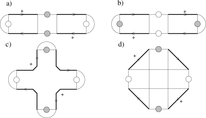
Figure 1: Diagrams representing the term $T_{4}$. See text for description.

In the case of the type $a$ (Fig. 1a), the leading order diagrams have ladder structures on the left and right of the middle part containing the matrix $C_{2}$. These contribute in orders $O(N)$ and $O(1)$,

$$T_{4}^{(a,l)}=\frac{2N_{1}^{2}N_{2}}{(N+1)^{2}}=\frac{2N_{1}^{2}N_{2}}{N^{2}}-\frac{4N_{1}^{2}N_{2}}{N^{3}}+O\left(\frac{1}{N}\right).$$

An other $O(1)$ correction comes from inserting a maximally crossed part into one of the ladders, resulting in

$$\delta T_{4}^{(a,mc)}=\frac{2N_{1}^{2}N_{2}}{N^{3}}\left(2-N\left({\mathcal{T}}C{\mathcal{T}}\right)_{\rho\sigma,\rho\sigma}\right).$$

The contribution from type $b$ (Fig. 1b) can be obtained from type $a$ by interchanging $N_{1}$ and $N_{2}$. In the case of type $c$ (Fig. 1c), the leading order diagrams have ladder structures attached to the central part, which can be an U-cycle of length two or a T-cycle representing ${\rm tr}\left(RR^{\dagger}RR^{\dagger}\right)$ with tr denoting channel tracePolianski . The corresponding contribution is

$$T_{4}^{(c,l)}=-\frac{2NN_{1}^{2}N_{2}^{2}}{(N+1)^{4}}=-\frac{2N_{1}^{2}N_{2}^{2}}{N^{3}}+\frac{8N_{1}^{2}N_{2}^{2}}{N^{4}}+O\left(\frac{1}{N}\right).$$

The higher order diagrams giving further $O(1)$ terms can be drawn again by inserting a maximally crossed part into one of the ladders or by opening the central part and putting the insertion between two neighboring ladders. Evaluating the diagrams we find

$$T_{4}^{(c,mc)}=-\frac{4N_{1}^{2}N_{2}}{N^{4}}\left(2-N\left({\mathcal{T}}C{\mathcal{T}}\right)_{\rho\sigma,\rho\sigma}\right).$$

Finally, as the contributions of type $d$ (Fig. 1d) are at most of order $O(1/N^{2})$, they can be disregarded in a weak localization calculation.

Collecting the contributions to $T_{4}$ and using (6) and (7), for the average shot noise power we find

$$\frac{\langle P\rangle}{P_{0}}=\frac{2N_{1}^{2}N_{2}^{2}}{N^{3}}+\frac{N_{1}N_{2}(N_{1}-N_{2})^{2}}{N^{3}}\left({\mathcal{T}}C{\mathcal{T}}\right)_{\rho\sigma,\rho\sigma},$$ (10)

which is the main result of our paper. Similarly to the case of the conductance, all the dependence on the magnetic fields and spin-orbit coupling is through the combination $\left({\mathcal{T}}C{\mathcal{T}}\right)_{\rho\sigma,\rho\sigma}$. The concrete expressions for $\left({\mathcal{T}}C{\mathcal{T}}\right)_{\rho\sigma,\rho\sigma}$ corresponding to the various symmetry class transitions can be found in Refs. BCH, ; CBF, . In the particular case of an orthogonal-unitary crossover the semiclassical prediction (1) is recovered.

Together with (7), the formula (10) indeed implies that the relation (3) holds for all the crossovers due to magnetic fields and spin-orbit coupling studied in the context of transport in chaotic quantum dots. This means that the first quantum correction to the ensemble averaged shot noise is related to the first quantum correction to the ensemble averaged mean current $\langle\overline{I}\rangle=\langle G\rangle V$ by a simple multiplication with a factor that (apart from a sign) depends only on the channel number asymmetry of the system. It would be interesting to know if there is a similar relation for higher dimensional disordered mesoscopic conductors.

In summary, we gave an RMT prediction for the average shot noise power as a function of magnetic field and spin-orbit coupling. Our result can be applied to the various crossovers ranging from the standard weak localization - weak antilocalization transition to the interpolation between the symmetry classes identified by Aleiner and FalkoAF . We found that the remarkably simple relation (3) between $\delta P$ and $\delta G$ persists for all of these crossovers. In the special case of an orthogonal-unitary transition we recover the semiclassical prediction of Braun et al.Braun .

We gratefully acknowledge discussions with C. W. J. Beenakker. This work is supported by E. C. Contract No. MRTN-CT-2003-504574.

References

- (1) C. W. J. Beenakker, C. Schönenberger, Physics Today, May 2003, page 37.
- (2) Ya. M. Blanter and M. Büttiker, Physics Reports 336, 1 (2000).
- (3) M. J. M. de Jong and C. W. J. Beenakker, Phys. Rev. B 46 13400 (1992).
- (4) A. M. S. Macêdo, Phys. Rev. B 49 1858 (1994) .
- (5) A. M. S. Macêdo and J. T. Chalker, Phys. Rev. B 49 4695 (1994).
- (6) A. M. S. Macêdo, Phys. Rev. Lett. 79 5098 (1997).
- (7) C. W. J. Beenakker, Rev. Mod. Phys. 69, 731 (1997).
- (8) P. Braun, S. Heusler, S. Müller and F. Haake, J. Phys. A: Math. Gen. 39, L159-L165 (2006).
- (9) Note that recently an entirely different mechanism was discovered, effective in the limit when the Ehrenfest time can exceed the dwell time, see Ossipov et. al, Europhys. Lett. 76, 115 (2006).
- (10) B.I.Halperin, A. Stern, Y. Oreg, J. N. H. J. Cremers, J. A. Folk and C. M. Marcus, Phys. Rev. Lett. 86, 2106 (2001).
- (11) I. L. Aleiner and V. I. Fal’ko, Phys. Rev. Lett. 87, 256801 (2001); 89, 079902(E) (2002).
- (12) P. W. Brouwer, J. N. H. J. Cremers, and B. I. Halperin, Phys. Rev. B 65, 081302 (2002).
- (13) J.H. Cremers, P.W. Brouwer, and V.I. Falko, Phys. Rev. B 68, 125329 (2003).
- (14) J.A.Folk, S. R. Patel, K. M. Birnbaum and C. M. Marcus, Phys. Rev. Lett. 86, 2102 (2001).
- (15) D. M. Zumbühl, J. B. Miller, C. M. Marcus, K. Campman, and A. C. Gossard, Phys. Rev. Lett. 89, 276803 (2002).
- (16) D. M. Zumbühl, J. B. Miller, D. Goldhaber-Gordon, C. M. Marcus, J. S. Harris, K. Campman, and A. C. Gossard, Phys. Rev. B. 72, 081305 (2005).
- (17) J. H. Bardarson, J. Tworzydlo and C. W. J. Beenakker, Phys. Rev. B. 72, 235305 (2005).
- (18) Ya. M. Blanter and E. V. Sukhorukov, Phys. Rev. Lett. 84, 1280 (2000).
- (19) O. Agam, I. Aleiner and A. Larkin, Phys. Rev. Lett.85, 3153 (2000).
- (20) R. G. Nazmitdinov, H.-S. Sim, H. Schomerus and I. Rotter, Phys. Rev. B 66, 241302(R) (2002).
- (21) P. G. Silvestrov, M. C. Goorden and C. W. J. Beenakker, Phys. Rev. B 67, 241301(R) (2003).
- (22) Ph. Jacquod and E. V. Sukhorukov, Phys. Rev. Lett. 92, 116801 (2004).
- (23) E. V. Sukhorukov and O. M. Bulashenko, Phys. Rev. Lett. 94, 116803 (2005).
- (24) F. Aigner, S. Rotter and J. Burgdörfer, Phys. Rev. Lett. 94, 216801 (2005).
- (25) S. Oberholzer, E. V. Sukhorukov, C. Strunk, C. Schönenberger, T. Heinzel and M. Holland, Phys. Rev. Lett. 86, 2114 (2001).
- (26) S. Oberholzer, E. V. Sukhorukov, C. Schönenberger, Nature (London) 415, 765 (2002).
- (27) D. V. Savin, H.-J. Sommers, Phys. Rev. B 73, 081307(R) (2006).
- (28) Z. Pluhar, H. A. Weidenmüller, J. A. Zuk, C. H. Lewenkopf, Phys. Rev. Lett. 73, 2115 (1994).
- (29) Z. Pluhar, H. A. Weidenmüller, J. A. Zuk, C. H. Lewenkopf, F. J. Wegner, Ann. of Phys. 243, 1 (1995).
- (30) K. M. Frahm, Europhys. Lett. 30 457 (1995).
- (31) S. Heusler, S. Müller, P. Braun, and F. Haake Phys. Rev. Lett 96, 066804 (2006).
- (32) V. A. Khlus, JETP 66, 1243 (1987).
- (33) G. B. Lesovik, JETP Lett. 49, 592 (1987).
- (34) M. Büttiker, Phys. Rev. Lett. 65, 2901 (1990).
- (35) P. W. Brouwer, K. M. Frahm, and C. W. J. Beenakker, Waves in Random Media 9, 91 (1999).
- (36) P. W. Brouwer and C. W. J. Beenakker, J. Math. Phys. 37, 4904 (1996).
- (37) M. L. Polianski, P. W. Brouwer, J. Phys. A: Math. Gen. 36, 3215 (2003).