Statistical Scattering of Waves in Disordered Waveguides: from Microscopic Potentials to Limiting Macroscopic Statistics

Abstract

We study the statistical properties of wave scattering in a disordered waveguide. The statistical properties of a “building block” of length $\delta L$ are derived from a potential model and used to find the evolution with length of the expectation value of physical quantities. In the potential model the scattering units consist of thin potential slices, idealized as delta slices, perpendicular to the longitudinal direction of the waveguide; the variation of the potential in the transverse direction may be arbitrary. The sets of parameters defining a given slice are taken to be statistically independent from those of any other slice and identically distributed. In the dense-weak-scattering limit, in which the potential slices are very weak and their linear density is very large, so that the resulting mean free paths are fixed, the corresponding statistical properties of the full waveguide depend only on the mean free paths and on no other property of the slice distribution. The universality that arises demonstrates the existence of a generalized central-limit theorem.

Our final result is a diffusion equation in the space of transfer matrices of our system, which describes the evolution with the length $L$ of the disordered waveguide of the transport properties of interest. In contrast to earlier publications, in the present analysis the energy of the incident particle is fully taken into account.

For one propagating mode, $N=1$, we have been able to solve the diffusion equation for a number of particular observables, and the solution is in excellent agreement with the results of microscopic calculations. In general, we have not succeeded in finding a solution of the diffusion equation. We have thus developed a numerical simulation, to be called “random walk in the transfer matrix space”, in which the universal statistical properties of a “building block” are first implemented numerically, and then the various building blocks are combined to find the statistical properties of the full waveguide. The reported results thus obtained (in which use was made of a “short-wavelength approximation”) are in very good agreement with those arising from truly microscopic calculations, for both bulk and surface disorder.

I Introduction

The statistical theory of certain complex wave interference phenomena, like the statistical fluctuations of transmission and reflection of waves, is of considerable interest in many fields of physics Ishimaru78 ; Rytov89 ; Nieto-V90 ; Altshuler91 ; Sheng95 ; carlo97 ; Imrybook ; Dattabook ; Alhassid ; mello-kumar ; WRM . In the literature one has contemplated situations in which such a complexity derives from the chaotic nature of the underlying classical dynamics, as in the case of chaotic microwave cavities and quantum dots, or from the quenched randomness of scattering potentials, as in the case of disordered conductors or, more in general, disordered waveguides. It is the latter domain that will interest us here.

In studies performed in such systems one has found remarkable statistical regularities, in the sense that the probability distribution for various macroscopic quantities involves a rather small number of relevant physical parameters, or scaling parameters, while the rest of the microscopic details serves as mere “scaffolding”. In Ref. mello_shapiro it was shown that a limiting distribution of physical quantities indeed arises in the so called dense-weak-scattering limit (DWSL) and within a particular class of models: the individual, microscopic, scattering units were defined through their transfer matrices and an “isotropic” distribution of their phases was assumed. The limiting distribution that was found constitutes a generalized central-limit theorem (CLT). Within this model only one relevant physical parameter occurs: the mean free path, which is the only property arising from the individual scattering units that survives in the DWSL. This is consistent with the scaling hypothesis proposed by E. Abrahams et al. gang_of_4 . (When abandoning the DWSL, two parameters were needed in Ref. mello_rmp to describe the conductance distribution.) The result found in Ref. mello_shapiro coincides with that of the maximum-entropy model that had been developed in Ref. mpk , which gives rise to a diffusion equation known as the DMPK equation (after Dorokhov dorokhov and Mello, Pereyra and Kumar mpk ), which can thus be interpreted as capturing the features arising from a CLT.

CLT’s associated with products of matrices had been studied earlier, as, for instance, in the well-known Oseledec theorem oseledec ; carlo97 ; the results of Refs. mello_shapiro ; mpk are consistent with this theorem in the localized regime.

In spite of the successes of the diffusion equation of Ref. mpk in the study of the conductance distribution carlo97 , that equation fails to give the proper description when the difference in behavior of the various modes becomes relevant. A clear example was given in Ref. UAM , where the conductance distribution was studied in the crossover region $\langle G\rangle\approx e^{2}/h$. For waveguides with bulk disorder the description is excellent, whereas for waveguides with surface disorder it is not satisfactory WRM ; UAM2 .

A class of limiting distributions wider than that of Ref. mello_shapiro was studied by one of the present authors and S. Tomsovic in Ref. mello_tomsovic (to be referred to as MT), in which the isotropy assumption of Ref. mello_shapiro was relaxed to a large extent. The DWSL played an essential role and the result was a more general CLT than that of Ref. mello_shapiro , expressed in terms of a generalized diffusion equation. The scaling parameters that appear in MT are the mean free paths (mfp’s) for the various scattering processes that may occur in the problem. When the various mfp’s can be represented by a single one, one encounters the same diffusion equation that was studied in Ref. mpk using a maximum-entropy model. Thus the MT model appears as a possible candidate to study, in the problem of waveguides with surface disorder, the influence of the specific scattering properties of the relevant modes.

The ideas of MT are further developed in the “Brownian-motion” model of Ref. houches : a waveguide of length $L$ is enlarged by adding a piece of thickness $\delta L$ [to be called a “building block” (BB)], small on a macroscopic scale but still containing many scatterers, which is likened to a Brownian particle which, in a time interval $\delta t$, small on a macroscopic scale, still suffers many collisions from the molecules of the surrounding medium. The transfer matrix for a BB is written as $M=I+\varepsilon$ and the independent parameters which $M$ depends upon are chosen so that $\varepsilon$ for the BB satisfies a number of properties, reminiscent of those of a Brownian particle:

$$\langle\varepsilon\rangle_{\delta L} = 0+O(\delta L^{2})$$ (1a)

$$\langle\varepsilon\varepsilon\rangle_{\delta L} = O(\delta L)\;,$$ (1b)

while higher moments of $\varepsilon$ behave as higher powers of $\delta L$ (see Eqs. (3.73) and (3.74) of Ref. houches ). The result of this analysis is the same diffusion equation as that of MT.

Though appealing the assumptions behind the Brownian-motion model of Ref. houches for the BB may be, they are, nevertheless, arbitrary. Of course, they can be deduced from the MT model for the more microscopic scattering units. However, even these have a certain degree of arbitrariness. It would be satisfactory if these models could be obtained in a unified way from a maximum-entropy “ansatz”: this, however, is not known to the present authors at this time.

The motivation of the present paper is to derive from a potential model the statistical properties of the BB and use them to find the “evolution” with length of the expectation value of physical quantities. Since the potential model will be introduced at the level of the individual scattering units, the approach to be presented here is, in a way, hybrid between the methods of MT and Ref. houches . We shall see that within the present model it is not strictly true that the individual transfer matrices (resulting from the individual potentials) for the various scatterers are identically distributed [see Eq. (36) below], as was assumed in MT, and this fact will be taken into account. The continuous limit is also treated here in a more satisfactory way than in MT, and the energy appears explicitly in the following presentation, in contrast to earlier publications. We believe that the present model is physically more complete than that of Ref. mpk ; it is also better founded than that of MT and Ref. houches , in the sense that there is a lesser degree of arbitrariness in the assumptions, although the resulting diffusion equation has a “structure” similar to the one obtained in MT and Ref. houches . Our diffusion equation covers situations not contemplated in these references: we shall find it suitable to study wave-transport problems in which the physics of the various modes is relevant; we shall also find a good description of the statistical properties of quantities that involve phases, which were not described at all in previous models. The reader is referred to Ref. mello_physicaA for a preliminary account of the results of the present paper.

The paper is organized as follows. In the next section we derive a Fokker-Planck equation for the “evolution” with the waveguide length $L$ of the expectation value of the physical quantities of interest. That equation represents the central result of the present paper and is given in Eq. (12), which we reproduce here for convenience:

$$\frac{\partial\left\langle F(\bm{M})\right\rangle_{L}}{\partial L}=\sum_{\begin{subarray}{c}ijhl\lambda\mu\\ abcd\alpha\beta\end{subarray}}D_{ab,cd}^{ij,hl}(k,L)\left\langle M_{b\alpha}^{j\lambda}\;M_{d\beta}^{l\mu}\;\frac{\partial^{2}F(\bm{M})}{\partial M_{a\alpha}^{i\lambda}\partial M_{c\beta}^{h\mu}}\right\rangle_{L}.$$ (2)

We notice that Eq. (2) contains no drift term and is thus a diffusion equation. The physical observable is denoted by $F(\bm{M})$, $\bm{M}$ being the transfer matrix of the sample of length $L$. The quantities $D_{ab,cd}^{ij,hl}(k,L)$ play the role of “diffusion coefficients”, which are defined in terms of the second moments of $\varepsilon$ for the BB in Eq. (62) below (see the term linear in $\delta L$) and are given explicitly in Eq. (63) in terms of the mean free paths. Notice that the diffusion coefficients depend on the energy ($\sim k^{2}$) and also on the length $L$ of the sample. The mean free paths depend only on the second moments of the potential intensity of the individual impurities [see Eq. (48)], higher moments being irrelevant for the diffusion equation: this is precisely what signals the existence of a CLT. In order to derive the diffusion equation (2) we need a statistical model for the building block (BB): this is derived in Sec. III using a potential model for the random impurities. Although the treatment of Sec. II is applicable to the orthogonal as well as to the unitary symmetry classes of Random-Matrix Theory ($\beta=1$ and $2$, respectively dyson ), the potential model developed in Sec. III assumes time-reversal invariance, i.e., $\beta=1$. Some of the specific relations derived there would have to be properly modified for the unitary case, $\beta=2$. The results of Sec. III which are needed for the derivation of the diffusion equation (2) have an intrinsic interest as well, since they can be used to describe the statistical scattering properties of thin slabs. The diffusion equation (2) is first derived for arbitrary energy, and only later the short-wavelength approximation (SWLA) is contemplated; it is in this latter limit that some of the results obtained earlier can be recovered. Needless to say, we have no general way of finding either analytically or numerically the solutions of the above diffusion equation. We thus give in Sec. IV.1 some simple examples in which the analytic solution could be found; in Sec. IV.2 we develop a procedure to simulate numerically the diffusion process in transfer-matrix space, and present some of the results that we have been able to obtain so far. The conclusions of this work are given in Sec. V. A number of appendices have been included, in which some of the specific calculations are carried out.

II Transport in q-1D disordered systems. The combination law and the Smoluchowsky equation. The diffusion equation

Consider a q-1D disordered system of uniform cross section, connected, at both ends, to clean waveguides that support $N$ open channels each. In the disordered region there is an underlying random potential to be specified later. In some applications we shall be concerned with a 2D waveguide with a width to be denoted by $W$.

The scattering properties of the system will be described by means of its transfer matrix $\bm{M}$, which can be written as

$$\bm{M}=\left[\begin{array}[]{ll}M^{11}&M^{12}\\ M^{21}&M^{22}\end{array}\right]\equiv\left[\begin{array}[]{ll}\alpha&\beta\\ \gamma&\delta\end{array}\right].$$ (3)

Each block $M^{ij}$ ($i=1,2$; $j=1,2$) in (3) is $N$-dimensional, so that $\bm{M}$ is $2N$-dimensional. (The block $M^{12}$ will occasionally be denoted by $\beta$, a symbol not to be confused with the index for universality classes in Random-Matrix Theory.) One particular matrix element of the $ij$ block will be designated as $M_{ab}^{ij}$, where $a,b\;(=1,\cdots,N)$ denote the channels. Some of the properties of the $\bm{M}$ matrix and its relation with the more conventional reflection and transmission amplitudes, which are elements of the $\bm{S}$ matrix, are summarized in App. A.

The transfer matrix $\bm{M}$ will be considered to belong to one of the basic symmetry classes introduced by Dyson in Quantum Mechanics dyson . Here we shall be only concerned with scalar waves, so that, in applications to quantum mechanics, we shall only have “spinless electrons”. In the “unitary” case, also denoted by $\beta=2$, the only restriction on $\bm{M}$ is flux conservation, which is expressed by the pseudo-unitarity condition, Eq. (120). In the “orthogonal” case ($\beta=1$), time-reversal invariance imposes the restriction given by Eq. (121). The “symplectic” case ($\beta=4$) associated with half-integral spin will not be considered here.

If the underlying potential has non-zero matrix elements between open and closed channels, the $2N$-dimensional $\bm{M}$ matrix depends on an “effective potential” which contains information on closed channels, as explained in App. B.

Consider now two non-overlapping scatterers. Their extended transfer matrices, $\tilde{\bm{M}}_{1}$ and $\tilde{\bm{M}}_{2}$ (which include open and closed channels, are infinite-dimensional and depend on the bare potential, as opposed to the effective one), have the multiplicativity property (see App. A.3)

$$\tilde{\bm{M}}=\tilde{\bm{M}}_{2}\tilde{\bm{M}}_{1}.$$ (4)

In past publications by one of the authors (PAM) (see, for instance, Ref. mello-kumar ), closed channels have been neglected in the matrix multiplication of successive scatterers. In numerical simulations WRM ; JJS_evanesc one sees that for individual configurations of the disordered system and in the calculation of the mean free path, the inclusion of closed channels is important. (In this paper, the expressions “closed channels” and “evanescent modes” will be taken as synonymous.) On the other hand, for the statistical fluctuations the conditions for neglecting the evanescent modes do not appear to be very stringent. For a given mean free path, the statistical properties of the different transport coefficients are found to be roughly independent of the number of evanescent modes (see also the discussion of the numerical simulations given in Sec. IV.2.3). In this article we shall thus follow the earlier approximation and write the resulting transfer matrix as the product of the individual open-channel transfer matrices.

Suppose we start with a system containing $n$ scattering units (to be defined at the beginning of Sec. III) and enlarge it by adding, on its right-hand side, say, a slab, to be called a building block (BB), containing $m$ scattering units. Designating by $\bm{M}^{(L)}$ the transfer matrix of the original system and by $\bm{M}^{(\delta L)}$ that of the BB, the resulting transfer matrix is

$$\bm{M}^{(L+\delta L)}=\bm{M}^{(\delta L)}\bm{M}^{(L)}.$$ (5)

We assume the BB to be of arbitrary thickness $\delta L$, and to contain many weak scatterers (see Fig. 1).

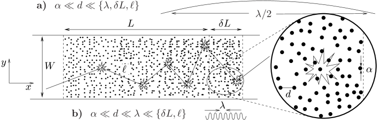
Figure 1: Schematic representation of a disordered wire and the building block (BB); (a) and (b) correspond to the different regimes (see Section III) defined by the inequalities given in Eqs. (13a) and (13b) (short-wavelength approximation (SWLA)), respectively.

Its transfer matrix $\bm{M}^{(\delta L)}$ will be written as

$$\bm{M}^{(\delta L)}=\bm{I}_{2N}+\bm{\varepsilon}.$$ (6)

The combination law for $\bm{M}$, Eq. (5), can be written as

$$\bm{M}^{(L+\delta L)} = \bm{M}^{(L)}+\delta\bm{M}$$ (7a)

$$= \bm{M}^{(L)}+\bm{\varepsilon M}^{(L)}.$$ (7b)

Consider now a function $F(\bm{M})$ of the $\bm{M}$ matrix, which we shall call an “observable”: it could be, for instance, the transmission amplitude $t_{ab}$, or the conductance $G$, which is proportional to the total transmission coefficient $T$. We are interested in the expectation value $\left\langle F(\bm{M})\right\rangle_{n}$ of such an observable for a system containing $n$ impurities. We first find below a recurrence relation with $n$ for that expectation value and then, in the continuous limit, we shall find the equation that governs the “evolution” of $\left\langle F(\bm{M})\right\rangle_{L}$ with increasing length $L$.

If we write a particular $\bm{M}$ matrix element as $M_{ab}^{ij}=\xi_{ab}^{ij}+i\eta_{ab}^{ij}$, we may consider the observable $F(\bm{M})$ as a function of all those $\xi_{ab}^{ij}$ and $\eta_{ab}^{ij}$ which are relevant for the universality class $\beta$ in question. For instance, in the orthogonal case ($\beta=1$), because of the TRI relation, Eq. (123), only the real and imaginary parts of the blocks $M_{ab}^{11}$ and $M_{ab}^{12}$ are relevant, while in the unitary case ($\beta=2$) the real and imaginary parts of the four blocks $M_{ab}^{ij}$ ($i=1,2$; $j=1,2$) are needed. Alternatively, we may consider $F(\bm{M})$ as a function of all the relevant $M_{ab}^{ij}$’s and their complex conjugates, a possibility which will be found more convenient in what follows. For $\beta=1$, Eq. (123) shows that this is equivalent to expressing $F(\bm{M})$ as a function of all the $M_{ab}^{ij}$ ($i=1,2$; $j=1,2$), enforcing Eq. (123) at the end, while for $\beta=2$ we need all the $M_{ab}^{ij}$ ($i=1,2$; $j=1,2$) and their complex conjugates. In what follows we shall restrict ourselves to the orthogonal case.

Writing the composition law for the $\bm{M}$ matrix as in Eq. (7), the expressions for the observable $F(\bm{M})$ before and after adding the building block are related by the Taylor expansion

$$F\left(\bm{M}^{(n+m)}\right)=F\left(\bm{M}^{(n)}+\delta\bm{M}\right)=F\left(\bm{M}^{(n)}\right)+\sum_{\begin{subarray}{c}i\lambda\\ a\alpha\end{subarray}}(\delta M_{a\alpha}^{i\lambda})\;\frac{\partial F\left(\bm{M}\right)}{\partial M_{a\alpha}^{i\lambda}}\Bigg{|}_{\bm{M}=\bm{M}^{(n)}}$$

$$\;\;\;\;\;\;\;+\frac{1}{2!}\;\sum_{\begin{subarray}{c}i\lambda h\mu\\ a\alpha c\beta\end{subarray}}(\delta M_{a\alpha}^{i\lambda})\;(\delta M_{c\beta}^{h\mu})\;\frac{\partial^{2}F\left(\bm{M}\right)}{\partial M_{a\alpha}^{i\lambda}\partial M_{c\beta}^{h\mu}}\Bigg{|}_{\bm{M}=\bm{M}^{(n)}}+\;\cdots\;,$$ (8)

where the lower indices $a,\alpha,\cdots$ on each $M$ indicate channels and run over the values $1,\cdots,N$, while the upper indices $i,\lambda,\cdots$ identify the block in Eq. (3) and take on the values $1,2$.

We take the expectation value of both sides of Eq. (8) with respect to the enlarged system containing $n+m$ scattering units and use Eq. (7), considering the two pieces $n$ and $m$ to be statistically independent. We find

$$\left\langle F(\bm{M})\right\rangle_{n+m}=\left\langle F(\bm{M})\right\rangle_{n}+\sum_{\begin{subarray}{c}ij\lambda\\ ab\alpha\end{subarray}}\left\langle\varepsilon_{ab}^{ij}\right\rangle_{m}\left\langle M_{b\alpha}^{j\lambda}\;\frac{\partial F(\bm{M})}{\partial M_{a\alpha}^{i\lambda}}\right\rangle_{n}$$

$$\;\;\;\;\;\;\;+\;\frac{1}{2!}\sum_{\begin{subarray}{c}ijhl\lambda\mu\\ abcd\alpha\beta\end{subarray}}\left\langle\varepsilon_{ab}^{ij}\;\varepsilon_{cd}^{hl}\right\rangle_{m}\left\langle M_{b\alpha}^{j\lambda}\;M_{d\beta}^{l\mu}\;\frac{\partial^{2}F(\bm{M})}{\partial M_{a\alpha}^{i\lambda}\;\partial M_{c\beta}^{h\mu}}\right\rangle_{n}\;+\;\cdots\;.$$ (9)

Here, $\left\langle\cdot\cdot\cdot\right\rangle_{n}$ denotes an average evaluated with the probability density for the transfer matrix of the original sample containing $n$ scattering units, i.e.,

$$\left\langle G(\bm{M})\right\rangle_{n}\equiv\left\langle G(\bm{M}^{(n)})\right\rangle.$$ (10)

A few comments are in order at this point. We recall that the various matrix elements $M_{ab}^{ij}$ are not independent: they are related by the pseudounitarity condition, Eq. (120), arising from flux conservation, and by Eq. (121), associated with time-reversal invariance. Of course, we can express the $M_{ab}^{ij}$’s in terms of independent parameters, like those occurring in the “polar representation” of the transfer matrix, and perform a Taylor expansion (similar to the one above) with respect to such independent parameters mello-kumar ; mpk . Here, just as in Ref. mello_tomsovic , we have found it simpler to perform the expansion with respect to the matrix elements $M_{ab}^{ij}$ themselves, as in Eq. (8), in the understanding that in the resulting expression (8) the $M_{ab}^{ij}$’s and $\delta M_{ab}^{ij}$’s have to be expressed in terms of independent parameters. The average appearing in Eq. (9) is thus performed with a probability density for such independent parameters. Since the latter depend on the underlying microscopic potentials, in this paper we shall not propose a model for the transfer matrix independent parameters, but rather for the microscopic potentials. (See also Ref. mello_tomsovic .)

The next step is to describe the problem in the dense-weak-scattering limit (DWSL) briefly described in the Introduction (and defined in Eqs. (50d) below), so that we can speak of the continuous length $L$ of the system and the length $\delta L$ of the BB. Eq. (9) becomes

$$\left\langle F(\bm{M})\right\rangle_{L+\delta L}=\left\langle F(\bm{M})\right\rangle_{L}+\sum_{\begin{subarray}{c}ij\lambda\\ ab\alpha\end{subarray}}\left\langle\varepsilon_{ab}^{ij}\right\rangle_{L,\delta L}\left\langle M_{b\alpha}^{j\lambda}\;\frac{\partial F(\bm{M})}{\partial M_{a\alpha}^{i\lambda}}\right\rangle_{L}$$

$$\;\;\;\;\;\;\;+\;\frac{1}{2!}\sum_{\begin{subarray}{c}ijhl\lambda\mu\\ abcd\alpha\beta\end{subarray}}\left\langle\varepsilon_{ab}^{ij}\;\varepsilon_{cd}^{hl}\right\rangle_{L,\delta L}\left\langle M_{b\alpha}^{j\lambda}\;M_{d\beta}^{l\mu}\;\frac{\partial^{2}F(\bm{M})}{\partial M_{a\alpha}^{i\lambda}\;\partial M_{c\beta}^{h\mu}}\right\rangle_{L}\;+\;\cdots\;.$$ (11)

To proceed, we need a statistical model for the BB. For this purpose, as we mentioned in the previous paragraph, a potential model is discussed in Sec. III, in which the BB is constructed as a collection of $m$ individual scattering units represented by delta-potential slices. It is found that the first moment of $\bm{\varepsilon}$ for the BB vanishes [see Eq. (41)], the second moments, in the DWSL, admit an expansion in powers of $\delta L$ starting with $\delta L$ itself (see Eq. (62), while higher moments behave as higher powers thereof (see the discussion following Eq. (186)). Also, the very important result emerges that the dependence on the cumulants of the potential higher than the second drops out in the DWSL. These results are reminiscent of the statistical behavior of the velocity increment of a Brownian particle during a time interval $\delta t$ during which many collisions from the surrounding medium have occurred chandra .

When the moments of the BB, evaluated in the DWSL, are substituted in Eq. (11), we obtain, on the r.h.s of that equation, a power series in $\delta L$. We also perform, on the l.h.s. of Eq. (11), a Taylor expansion of $\left\langle F(\bm{M})\right\rangle_{L+\delta L}$ in powers of $\delta L$ around the “initial” value $\left\langle F(\bm{M})\right\rangle_{L}$. We can then identify the coefficients of the various powers of $\delta L$ on the two sides of the equation. In particular, the coefficients of $\delta L$ give the diffusion equation

$$\frac{\partial\left\langle F(\bm{M})\right\rangle_{L}}{\partial L}=\sum_{\begin{subarray}{c}ijhl\lambda\mu\\ abcd\alpha\beta\end{subarray}}D_{ab,cd}^{ij,hl}(k,L)\left\langle M_{b\alpha}^{j\lambda}\;M_{d\beta}^{l\mu}\;\frac{\partial^{2}F(\bm{M})}{\partial M_{a\alpha}^{i\lambda}\partial M_{c\beta}^{h\mu}}\right\rangle_{L}.$$ (12)

The quantities $D_{ab,cd}^{ij,hl}(k,L)$ play the role of “diffusion coefficients”: they are defined in Eq. (62) below as proportional to the coefficient of the linear term in an expansion in powers of $\delta L$ of the second moment of $\varepsilon$ for the BB and are given explicitly in Eq. (63) in terms of the mean free paths. The diffusion coefficients depend on the energy ($\sim k^{2}$) and also on the length $L$ of the sample.

We remark that, just as the coefficients of $\delta L$ in Eq. (11) are expressible in terms of the mfp’s, the coefficients of higher-order terms in $\delta L$ have a similar property, because the contribution of higher moments becomes irrelevant in the DWSL. Equating the coefficients of such higher-order terms on both sides of Eq. (11) we obtain results which could be derived from the diffusion equation (12) by successive differentiations. (See comment right after Eq. (67).)

In the potential model discussed in the next section only the orthogonal case, $\beta=1$, is contemplated. We expect a similar behavior for the unitary class, $\beta=2$, although we do not have at the present moment the specific expression for each diffusion coefficient in this case.

Eq. (12) represents the central result of the present paper. It depends only on the mean free paths which, in turn, depend only on the second moments of the individual delta-potential strengths [Eq. (48)]. The fact that cumulants of the potential higher than the second are irrelevant in the end signals the existence of a generalized CLT: once the mfp’s are specified, the limiting equation (12) is universal, i.e., independent of other details of the microscopic statistics.

III Statistical Properties of the Building Block

In the present section we investigate the statistical scattering properties of the BB which was used in Sec. II to build a disordered system with a q1D geometry (see Fig. 1).

Suppose that we model the scatterers constituting the BB by a sequence of thin slices (the scattering units referred to right above Eq. (5)) of cross section $W^{D-1}$ ($D$ being the dimensionality of the waveguide). From now on we denote the thickness of the slices by $2\alpha$ and their separation by $d$. (See Fig. 2 below. Notice that in Fig. 1 the same symbols refer to individual scatterers; here, a slice may contain one or more of the individual scatterers shown in Fig. 1.) The statistical properties of the potential slices will be specified below (see Sec. III.2.1). Inside $2\alpha$, the $r$-th scattering slice is described by the potential $V_{r}(x,\bm{y})$. We denote by $x$ the coordinate along the waveguide and by $\bm{y}$ the coordinates in the transverse direction. The distance $d$ between slices is taken to be much larger than $\alpha$, but much smaller than the wavelength $\lambda$ of the incident wave and the thickness $\delta L$ of the BB. Initially we do not specify the ratio of the wavelength $\lambda$ to $\delta L$ or the mean-free-path $\ell$ (to be defined later), so we shall start out constructing the BB as a collection of $m$ thin slices satisfying the inequalities

$$\alpha\ll d\ll\{\lambda,\delta L,\ell\}.$$ (13a)

Later on, in section III.4, we shall find it advantageous to study a second regime, in which $$\delta L L \ell$$ (and hence any final ) and contain many wavelengths, i.e.,

$$\alpha\ll d\ll\lambda\ll\{\delta L,\ell\}\;,$$ (13b)

corresponding to what we shall call the short-wavelength approximation (SWLA).

In principle we have no restriction on the dimensionality $D$ of the waveguide; however, to be specific, we shall restrict the discussion to two-dimensional waveguides with uniform width $W$. As we already indicated, in the potential model to be presented below we shall be concerned with the orthogonal, or $\beta=1$, symmetry class only.

III.1 Properties of a single scattering slice

Consider a single scattering slice with potential $V(x,y)=\hbar^{2}U(x,y)/(2m)$, centered at the origin of coordinates $x=0$, and let $[U(x)]_{ab}$ be the matrix elements of $U(x,y)$ with respect to the “transverse” states $\chi_{a}(y)$ of the waveguide, i.e.,

$$[U(x)]_{ab}=\int_{0}^{W}\chi_{a}(y)U(x,y)\chi_{b}(y)dy,$$ (14)

with

$$\chi_{a}(y)=\sqrt{\frac{2}{W}}\sin\frac{\pi ay}{W},$$ (15)

$a$ being an integer. Under the conditions

$$k\alpha \ll 1$$ (16a)

$$K_{ab}\alpha \ll 1,$$ (16b)

where $k=2\pi/\lambda=\sqrt{2mE}/\hbar$ and

$$K_{ab}^{2}=|U_{ab}|\equiv\big{|}[U(0)]_{ab}\big{|},$$ (17)

we speak of a thin scatterer (a thin barrier or well) and the dependence of the potential across the thickness $2\alpha$ is neglected. On the other hand, the quantity

$$2\alpha\cdot U_{ab}\equiv u_{ab}$$ (18)

(which has dimensions of $k$) is arbitrary. Such a scatterer can be well approximated by the “delta potential”

$$U(x,y) = u(y)\delta(x),$$ (19a)

$$\left[U(x)\right]_{ab} = u_{ab}\;\delta(x)\;,$$ (19b)

obtained formally taking the limits

$$|U_{ab}| \rightarrow \infty,$$ (20a)

$$\alpha \rightarrow 0,$$ (20b)

in such a way that the quantity $u_{ab}$ of Eq. (18) stays fixed. From the inequalities (13) we see that the range $2\alpha$ of the potential is the smallest length scale in the problem: the limit (20b) is the extreme idealization of this situation.

Eqs. (19) define a delta-slice potential centered at the origin of coordinates. The potential produced by the $r$-th delta slice, centered at $x=x_{r}$, is written as

$$U_{r}(x,y) = u_{r}(y)\delta(x-x_{r})$$ (21a)

$$\left[U_{r}(x)\right]_{ab} = (u_{r})_{ab}\;\delta(x-x_{r}).$$ (21b)

We remind the reader that $U_{r}(x,y)$ has dimensions of $k^{2}$, whereas $u_{r}(y)$ and $(u_{r})_{ab}$ have dimensions of $k$.

A particle scattered by the potential of Eq. (19) inside the waveguide is described by the wave function

$$\psi(x,y)=\sum_{a=1}^{\infty}\left[\psi(x)\right]_{a}\chi_{a}(y),$$ (22)

which satisfies Schrödinger’s equation; its components $\left[\psi(x)\right]_{a}$ satisfy the coupled equations

$$\left(\frac{\partial^{2}}{\partial x^{2}}+k_{a}^{2}\right)\left[\psi(x)\right]_{a} = \sum_{b=1}^{\infty}\left[\psi(x)\right]_{b}{(u_{r})}_{ab}\delta(x-x_{r})\;,\hskip 28.45274pt1\leq a\leq N$$ (23a)

$$\left(\frac{\partial^{2}}{\partial x^{2}}-\kappa_{a}^{2}\right)\left[\psi(x)\right]_{a} = \sum_{b=1}^{\infty}\left[\psi(x)\right]_{b}{(u_{r})}_{ab}\delta(x-x_{r})\;,\hskip 28.45274pta\geq N+1.$$ (23b)

Eq. (23a) refers to open channels and Eq. (23b) to closed ones. The quantity $k_{a}$, defined by the relation

$$k_{a}^{2}=k^{2}-\left(\frac{\pi a}{W}\right)^{2},$$ (24)

is the “longitudinal” momentum for the open channel $a$, with the replacement $k_{a}\Rightarrow i\kappa_{a}$ for closed channels mello-kumar . Notice that if $N\pi<kW<(N+1)\pi$, the problem admits precisely $N$ open channels.

The open-channel, $2N$-dimensional, transfer matrix $\bm{M}$ (that relates open-channel amplitudes on both sides of the potential) for the $r$-th slice, to be designated by $\bm{M}_{r}$, will be written as

$$\bm{M}_{r}=\left[\begin{array}[]{cc}M^{11}_{r}&M^{12}_{r}\\ \left[M^{12}_{r}\right]^{*}&\left[M^{11}_{r}\right]^{*}\end{array}\right]\equiv\bm{I}_{2N}+\bm{\epsilon}_{r}.$$ (25)

Since, eventually, we shall be interested in the limit of weak scatterers in which $\bm{M}_{r}$ is close to the unit matrix, we have introduced the difference $\bm{\epsilon}_{r}$ between $\bm{M}_{r}$ and the $2N$-dimensional unit matrix $\bm{I}_{2N}$. In the above equation we have taken into account explicitly the fact that our system obeys time-reversal invariance (see App. A). The $11$ and $12$ blocks of the matrix $\epsilon_{r}$ are given by

$$(\epsilon_{r})_{ab}^{11} = -i(\hat{v}_{r})_{ab}e^{-i(k_{a}-k_{b})x_{r}}\equiv(\hat{v}_{r})_{ab}(\vartheta_{r})^{11}_{ab}$$ (26a)

$$(\epsilon_{r})_{ab}^{12} = -i(\hat{v}_{r})_{ab}e^{-i(k_{a}+k_{b})x_{r}}\equiv(\hat{v}_{r})_{ab}(\vartheta_{r})^{12}_{ab}\;,$$ (26b)

where $a$ and $b$ label the open channels and thus run from $1$ to $N$. We have defined

$$(\vartheta_{r})_{ab}^{jl}=(\vartheta(x_{r}))_{ab}^{jl}=i(-)^{j}e^{i[(-)^{j}k_{a}+(-)^{l+1}k_{b}]x_{r}}$$ (27)

and we have introduced the real quantities

$$(\hat{v}_{r})_{ab}=\frac{(\hat{u}_{r})_{ab}}{2\sqrt{k_{a}k_{b}}}\;,$$ (28)

where, as explained in App. B, $(\hat{u}_{r})_{ab}$ is an “effective” potential strength that takes into account transitions to closed channels [see also Ref. mello-kumar , Eq. (3.134)].

In the above equations the strength of the various scatterers is arbitrary. As we already indicated, we shall be interested in the situation of weak scatterers, defined by the inequality

$$|(\hat{u}_{r})_{ab}|\ll\sqrt{k_{a}k_{b}}\;,$$ (29)

which has to be added to the inequalities (13) in order to complete the specification of the physical regime.

III.2 Construction of the Building Block. The regime (13a).

III.2.1 The statistical model

The BB is assumed, for the time being, centered at $x=0$. For the application to Eq. (11) the BB will have to be translated to the interval $(L,L+\delta L)$; this will be done in Sec. III.3. The BB is constructed from $m$ delta slices located at the positions $x_{r}$ (see Fig. 2), i.e., assuming $m$ to be odd,

$$x_{r} = rd$$ (30a)

$$r = -\frac{m-1}{2},\cdots,0,\cdots,\frac{m-1}{2}$$ (30b)

$$\delta L = (m-1)d,$$ (30c)

where $d$ denotes the distance between successive slices and $\delta L$ the thickness of the BB.

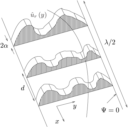
Figure 2: Schematic representation of the construction of the building block (BB) as a collection of “thin potential slices”.

The $m$ potentials $\hat{u}_{r}(y)$, $r=1,\cdots,m$, are assumed to be statistically independent and identically distributed. We indicate the $p$-th moments of the individual $\hat{u}_{r}(y)$’s and $\hat{v}_{r}(y)$ (which are related by the definition (28)) as

$$\mu_{p}^{(u)}(a_{1}b_{1},a_{2}b_{2},\cdots,a_{p}b_{p})=\Big{\langle}(\hat{u}_{r})_{a_{1}b_{1}}(\hat{u}_{r})_{a_{2}b_{2}}\cdots(\hat{u}_{r})_{a_{p}b_{p}}\Big{\rangle}$$ (31a)

$$\mu_{p}^{(v)}(a_{1}b_{1},a_{2}b_{2},\cdots,a_{p}b_{p})=\Big{\langle}(\hat{v}_{r})_{a_{1}b_{1}}(\hat{v}_{r})_{a_{2}b_{2}}\cdots(\hat{v}_{r})_{a_{p}b_{p}}\Big{\rangle}.$$ (31b)

We assume, for simplicity, that all odd moments vanish, i.e.,

$$\mu_{2t+1}^{(u)}(a_{1}b_{1},a_{2}b_{2},\cdots,a_{2t+1}b_{2t+1})=0.$$ (32)

We thus have

$$\langle(\hat{u}_{r})_{ab}\rangle = \mu_{1}^{(u)}(ab)=0$$ (33a)

$$\Big{\langle}(\hat{u}_{r})_{ab}(\hat{u}_{s})_{cd}\Big{\rangle} = \mu_{2}^{(u)}(ab,cd)\;\delta_{rs}\;$$ (33b)

$$\cdots\;\;$$

and similarly for the $\hat{v}_{r}$’s. It is useful to introduce the correlation coefficient between the matrix elements $(\hat{u}_{r})_{ab}$ and $(\hat{u}_{r})_{cd}$, (which coincides with the correlation coefficient between $(\hat{v}_{r})_{ab}$ and $(\hat{v}_{r})_{cd}$) as

$$C(ab,cd)=\frac{\mu_{2}^{(u)}(ab,cd)}{[\mu_{2}^{(u)}(ab)\mu_{2}^{(u)}(cd)]^{1/2}}=\frac{\mu_{2}^{(v)}(ab,cd)}{[\mu_{2}^{(v)}(ab)\mu_{2}^{(v)}(cd)]^{1/2}},$$ (34)

where $\mu_{2}^{(v)}(ab)\equiv\mu_{2}^{(v)}(ab,ab)$ denotes the variance of $(\hat{v}_{r})_{ab}$ (recall that $\mu_{1}^{(v)}(ab)=0$). For even moments higher than the second we do not make, at this point, any special assumption; a particular scaling law will be assumed in Eq. (51) below.

From the statistics of the $(\hat{u}_{r})_{ab}$’s (and $(\hat{v}_{r})_{ab}$’s) we can find the statistics of the $({\epsilon}_{r})_{ab}^{ij}$, using the relations (26). For instance, we find that the first moment of $({\epsilon}_{r})_{ab}^{ij}$ vanishes, i.e.,

$$\Big{\langle}(\epsilon_{r})_{ab}^{ij}\Big{\rangle}=0$$ (35)

and that the second moments can be written as

$$\Big{\langle}(\epsilon_{r})_{ab}^{ij}(\epsilon_{s})_{cd}^{hl}\Big{\rangle}=\mu_{2}^{(v)}(ab,cd)\left[(\vartheta_{r})_{ab}^{ij}(\vartheta_{r})_{cd}^{hl}\right]\delta_{rs},$$ (36)

where $(\vartheta_{r})_{ab}^{ij}$ was defined in Eqs. (26) and (27). The individual transfer matrices depend on the slice position $x_{r}$ and, as a consequence, they are not identically distributed.

III.2.2 The transfer matrix for the Building Block. Its first and second moments

The transfer matrix for the total sequence of $m$ delta slices is given by

$$\bm{M}^{(m)} = \bm{M}_{m}\bm{M}_{m-1}\cdots\bm{M}_{1}$$ (37a)

$$= \left(\bm{I}_{2N}+\bm{\epsilon}_{m}\right)\left(\bm{I}_{2N}+\bm{\epsilon}_{m-1}\right)\cdots\left(\bm{I}_{2N}+\bm{\epsilon}_{1}\right)$$ (37c)

$$= \bm{I}_{2N}+\sum_{r}\bm{\epsilon}_{r}+\sum_{r_{1}>r_{2}}\bm{\epsilon}_{r_{1}}\bm{\epsilon}_{r_{2}}+\cdots$$

$$\cdots+\sum_{r_{1}>...>r_{\mu}}\bm{\epsilon}_{r_{1}}\cdots\bm{\epsilon}_{r_{\mu}}+\cdots$$

$$\equiv \bm{I}_{2N}+\bm{\varepsilon}.$$ (37d)

The last line defines the matrix $\bm{\varepsilon}$ [that was already introduced in Eq. (6)] by which the total transfer matrix $\bm{M}$ of the BB differs from the unit matrix $\bm{I}_{2N}$; it is given by

$$\bm{\varepsilon} = \sum_{r}\bm{\epsilon}_{r}+\sum_{r_{1}>r_{2}}\bm{\epsilon}_{r_{1}}\bm{\epsilon}_{r_{2}}+\cdots+\sum_{r_{1}>...>r_{\mu}}\bm{\epsilon}_{r_{1}}\cdots\bm{\epsilon}_{r_{\mu}}+\cdots.$$ (38a)

$$\equiv \sum_{\mu=1}^{m}\bm{\varepsilon}^{(\mu)},$$ (38b)

where the last line defines the contribution to $\bm{\varepsilon}$ of order $\mu$ in the individual $\epsilon_{r}$’s. Our aim is to find the statistical properties –in particular the moments– of the matrix $\bm{\varepsilon}$. In the future we shall use the notation $\left\langle\cdots\right\rangle_{\delta L}$ to indicate an average associated with the BB, i.e.,

$$\left\langle G(\bm{M})\right\rangle_{\delta L}\equiv\left\langle G(\bm{M}^{(m)})\right\rangle,$$ (39)

just as in Eq. (10). For the average of $\bm{M}$ we trivially find, from Eqs. (37a), (37c) and the fact the various $\epsilon_{r}$’ are statistically independent and average to zero [Eq. (35)],

$$\left\langle\bm{M}\right\rangle_{\delta L}=\left\langle\bm{M}_{m}\right\rangle\cdots\left\langle\bm{M}_{1}\right\rangle=I_{2N}.$$ (40)

Thus Eq. (37d) implies that the first moment of $\bm{\varepsilon}$ vanishes, i.e.,

$$\left\langle\bm{\varepsilon}\right\rangle_{\delta L}=0,$$ (41)

as could also have been obtained by averaging Eq. (38) directly:

$$\left\langle\bm{\varepsilon}\right\rangle_{\delta L} = \sum_{\mu=1}^{m}\left\langle\bm{\varepsilon}^{(\mu)}\right\rangle_{\delta L}$$

$$= \sum_{r}\left\langle\bm{\epsilon}_{r}\right\rangle+\sum_{r_{1}>r_{2}}\left\langle\bm{\epsilon}_{r_{1}}\bm{\epsilon}_{r_{2}}\right\rangle+\cdots+\sum_{r_{1}>...>r_{\mu}}\left\langle\bm{\epsilon}_{r_{1}}\cdots\bm{\epsilon}_{r_{\mu}}\right\rangle+\cdots$$

$$= 0.$$ (42b)

For the second moments of $\varepsilon$ we have, from Eq. (38b)

$$\left\langle\varepsilon_{ab}^{ij}\varepsilon_{cd}^{hl}\right\rangle_{\delta L} = \sum_{\mu,\mu^{\prime}=1}^{m}\left\langle\left[\varepsilon^{(\mu)}\right]_{ab}^{ij}\left[\varepsilon^{(\mu^{\prime})}\right]_{cd}^{hl}\right\rangle_{\delta L}$$ (43a)

$$= \left\langle\left[\varepsilon^{(1)}\right]_{ab}^{ij}\left[\varepsilon^{(1)}\right]_{cd}^{hl}\right\rangle_{\delta L}$$

$$+ \left\langle\left[\varepsilon^{(1)}\right]_{ab}^{ij}\left[\varepsilon^{(2)}\right]_{cd}^{hl}\right\rangle_{L^{\prime}}+\left\langle\left[\varepsilon^{(2)}\right]_{ab}^{ij}\left[\varepsilon^{(1)}\right]_{cd}^{hl}\right\rangle_{\delta L}$$ (43b)

$$+ \left\langle\left[\varepsilon^{(2)}\right]_{ab}^{ij}\left[\varepsilon^{(2)}\right]_{cd}^{hl}\right\rangle_{\delta L}+\left\langle\left[\varepsilon^{(3)}\right]_{ab}^{ij}\left[\varepsilon^{(1)}\right]_{cd}^{hl}\right\rangle_{\delta L}+\left\langle\left[\varepsilon^{(1)}\right]_{ab}^{ij}\left[\varepsilon^{(3)}\right]_{cd}^{hl}\right\rangle_{\delta L}$$

$$+ \cdots.$$

The second line, Eq. (43a), is second order in the individual $[\epsilon_{r}]_{ab}^{ij}$ and hence in the potentials $(\hat{v}_{r})_{ab}$, and the successive lines are higher order in these quantities.

The second-order term in the second-moment expansion, Eq. (43a)

The second-order term, Eq. (43a), in the second moment expansion can be written using Eqs. (38) and (36) as

$$\left\langle\left[\varepsilon^{(1)}\right]_{ab}^{ij}\left[\varepsilon^{(1)}\right]_{cd}^{hl}\right\rangle_{\delta L} = \sum_{r,s}\left\langle(\epsilon_{r})_{ab}^{ij}(\epsilon_{s})_{cd}^{hl}\right\rangle$$ (44a)

$$= \sum_{r,s}\langle(\hat{v}_{r})_{ab}(\hat{v}_{s})_{cd}\rangle\left[(\vartheta_{r})_{ab}^{ij}(\vartheta_{s})_{cd}^{hl}\right]$$ (44b)

$$= \frac{\mu_{2}^{(v)}(ab,cd)}{d}\sum_{r}\left[(\vartheta_{r})_{ab}^{ij}(\vartheta_{r})_{cd}^{hl}\right]\cdot d.$$ (44c)

From the definition of the correlation coefficient between pairs of matrix elements, Eq. (34), we can write the fraction in Eq. (44c) as

$$\frac{\mu_{2}^{(v)}(ab,cd)}{d}=C(ab,cd)\left[\frac{\mu_{2}^{(v)}(ab)}{d}\;\frac{\mu_{2}^{(v)}(cd)}{d}\right]^{1/2}\equiv\frac{C(ab,cd)}{\sqrt{\ell_{ab}(k)\;\ell_{cd}(k)}}\;.$$ (45)

Here we have used the standard definition of the mean free path (mfp) $\ell_{ab}$ associated with the incoherent sum of reflections from channel $b$ to $a$ from a sequence of $\nu=1/d$ scatterers per unit length, i.e.,

$$\frac{1}{\ell_{ab}(k)}=\nu\Big{\langle}\left|(r_{1}(k))_{ab}\right|^{2}\Big{\rangle},$$ (46)

together with the fact that the average reflection coefficient for a delta slice is $r$-independent and approximately given, in the weak-scattering regime, Eq. (29), by [see Eqs. (124), (25) and (26)]

$$\Big{\langle}|(r_{1})_{ab}|^{2}\Big{\rangle}\approx\Big{\langle}[(\hat{v}_{1})_{ab}]^{2}\Big{\rangle}.$$ (47)

We can write the following equivalent expressions for the inverse mfp:

$$\frac{1}{\ell_{ab}(k)}=\nu\mu_{2}^{(v)}(ab)=\frac{\mu_{2}^{(v)}(ab)}{d}=\frac{\mu_{2}^{(u)}(ab)}{4k_{a}k_{b}d}\equiv\frac{\tilde{\mu}_{2}^{(u)}(ab)}{4k_{a}k_{b}}.$$ (48)

where the energy dependence of the mfp is exhibited explicitly. In the last member of the above equation we have defined the quantity $\tilde{\mu}_{2}^{(u)}(ab)$ as

$$\tilde{\mu}_{2}^{(u)}(ab)=\frac{\mu_{2}^{(u)}(ab)}{d}\;.$$ (49)

Since our delta slice is spatially symmetric in the $x$ direction, we have the same result for the mfp for the transmission, out of the incident flux, from channel $b$ to channel $a$. Within the present model there is thus no distinction between the so called transport and scattering mfp’s Ziman .

We now turn to the summation in Eq. (44c). We shall evaluate it in the dense-weak-scattering limit (DWSL) which we now define (see Eqs. (50d) below). This limit was already referred to in Secs. I and II. Within the regime defined by the inequalities (13a) we have already considered $\alpha$ as the smallest length scale occurring in the problem and simplified the situation by literally taking the limit $\alpha\to 0$ [Eq. (20b)]. With regards to the next length scale in our regime, i.e., the distance $d$ between successive scattering slices, we shall again be interested in a simplifying limit. For a fixed energy (and hence fixed $\lambda$), fixed $\delta L$ and mfp’s, it will be convenient to take the continuous limit

$$d \to 0$$ (50a)

$$m \to \infty,$$ (50b)

in such a way that

$$md=\delta L$$ (50c)

remains fixed. In order to keep the mfp’s $$\ell_{ab}$$ of Eq. (48) finite, we carry to an extreme the weak-scattering condition (29) and, for a fixed energy, take the limit in which the individual scattering units become infinitely weak, i.e.,

$$\mu_{2}^{(u)}(ab)\to 0,$$ (50d)

in such a way that, together with $d\to 0$, Eq. (50a), the ratio $\tilde{\mu}_{2}^{(u)}(ab)$ of Eq. (49), and hence the $\ell_{ab}(k)$ of Eq. (48), remain fixed. This limit has to be considered as the extreme idealization of the inequality (29) and of the inequality $d\ll\{\lambda,\delta L,\ell\}$ of (13a) for fixed energy, $\delta L$ and mfp’s.

We have already assumed in Eq. (32) that all the odd moments of $\hat{u}$ and $\hat{v}$ vanish. We shall now assume that the even moments, Eq. (31) with $p=2t$, scale with $d$ as

$$\mu_{2t}^{(u)}(a_{1}b_{1},\cdots,a_{2t}b_{2t})=d^{t}\;\tilde{\mu}_{2t}^{(u)}(a_{1}b_{1},\cdots,a_{2t}b_{2t}),$$ (51)

$\tilde{\mu}_{2t}^{(u)}(a_{1}b_{1},\cdots,a_{2t}b_{2t})$ being independent of $d$, with a similar expression for $\mu_{2t}^{(v)}(a_{1}b_{1},\cdots,a_{2t}b_{2t})$. Eq. (49) is the particular case of this last equation for $t=1$.

In the DWSL, the $\sum_{r}$ appearing in Eq. (44c) tends to an integral, which we denote by

$$\Delta_{ab,cd}^{ij,hl}(k,\delta L) \equiv \lim_{DWS}\sum_{r}\left[(\vartheta_{r})_{ab}^{ij}(\vartheta_{r})_{cd}^{hl}\right]\cdot d$$ (52)

$$= \int_{-\delta L/2}^{\delta L/2}\vartheta_{ab}^{ij}(x)\vartheta_{cd}^{hl}(x)dx\;,$$

where $\vartheta_{ab}^{ij}(x)$ is given by Eq. (27) with $x_{r}$ replaced by $x$. We find explicitly

$$\Delta_{ab,cd}^{ij,hl}(k,\delta L)=(-)^{i+h+1}\frac{\sin\frac{K_{ab,cd}^{ij,hl}\;\delta L}{2}}{\frac{K_{ab,cd}^{ij,hl}}{2}}\;,$$ (53)

a quantity with dimensions of length, $K_{ab,cd}^{ij,hl}$ being given by

$$K_{ab,cd}^{ij,hl}=(-1)^{i}k_{a}+(-1)^{j+1}k_{b}+(-1)^{h}k_{c}+(-1)^{l+1}k_{d}.$$ (54)

From Eq. (54), and using the notation of Eq. (127), we readily find the symmetry relations

$$K_{ab,cd}^{ij,hl}=K_{cd,ab}^{hl,ij}=-K_{ab,cd}^{\bar{i}\bar{j},\bar{h}\bar{l}}\;,$$ (55)

so that

$$\Delta_{ab,cd}^{ij,hl}(k,\delta L)=\Delta_{cd,ab}^{hl,ij}(k,\delta L)=\Delta_{ab,cd}^{\bar{i}\bar{j},\bar{h}\bar{l}}(k,\delta L)\;.$$ (56)

We thus have, for the expression (44) in the DWSL:

$$\lim_{DWS}\left\langle\left[\varepsilon^{(1)}\right]_{ab}^{ij}\left[\varepsilon^{(1)}\right]_{cd}^{kl}\right\rangle_{\delta L}=\frac{C(ab,cd)}{\sqrt{\ell_{ab}(k)\ell_{cd}(k)}}\Delta_{ab,cd}^{ij,hl}(k,\delta L)\;,$$ (57)

a result valid for arbitrary $k$ and $\delta L$.

For the application to Eq. (11) we shall need the expansion of the moments of $\varepsilon$ in powers of $\delta L$, with the BB translated to the interval $(L,L+\delta L)$; this will be done in Sec. III.3 below. For the time being we perform that expansion, for simplicity, with the BB centered at the origin. We see from Eq. (53) that the leading term of $\Delta_{ab,cd}^{ij,hl}(k,\delta L)$ in an expansion in powers of $\delta L$ is linear in $\delta L$ [as is obvious from the integral definition itself, Eq. (52)], i.e.,

$$\Delta_{ab,cd}^{ij,hl}(k,\delta L)=(-)^{i+h+1}\delta L+O(\delta L)^{2}.$$ (58)

As a result, Eq. (57) shows that the leading term in an expansion in powers of $\delta L$ of the second-order contribution to the second moments of $\varepsilon$ for the BB behaves, in the DWSL, as

$$\lim_{DWS}\left\langle\left[\varepsilon^{(1)}\right]_{ab}^{ij}\left[\varepsilon^{(1)}\right]_{cd}^{hl}\right\rangle_{\delta L}=(-)^{i+h+1}\frac{C(ab,cd)}{\sqrt{\ell_{ab}(k)\ell_{cd}(k)}}\delta L+O(\delta L)^{2}\;.$$ (59)

The fourth-order term in the second-moment expansion, Eq. (43)

A similar analysis is performed in App. C, Eq. (LABEL:vareps(2)vareps(2)_DWSL), for the fourth-order contribution to the second moments of $\varepsilon$, Eq. (43): it is shown that the leading term of such a quantity, in an expansion in powers of $\delta L$, behaves, in the DWSL, as $\left(\delta L/\ell\right)^{2}$, where $\ell$ denotes a typical mfp [see Eq. (165)]. From this result and Eq. (59) we thus have

$$\lim_{DWS}\left\langle\varepsilon_{ab}^{ij}\varepsilon_{cd}^{hl}\right\rangle_{\delta L}=(-)^{i+h+1}\frac{C(ab,cd)}{\sqrt{\ell_{ab}(k)\ell_{cd}(k)}}\delta L+O(\delta L)^{2}\;.$$ (60)

The analysis of the two above particular cases is generalized to arbitrary moments in App. D. For an even moment ($p=2t$) in the DWSL, the lowest-order term in Eq. (168) (this term is of order $2t$ in the $\hat{v}_{r}$’s) has a leading term in an expansion in powers of $\delta L$ which behaves as $(\delta L/\ell)^{t}$. Higher-order terms in (168) are higher order in $\delta L$. Also, the dependence on the cumulants of the potential higher than the second drops out in the DWSL. The contribution to the second moments obtained above, Eq. (60), represents, for $t=1$, a particular case of this general result. For an odd moment ($p=2t+1$), the corresponding term behaves as $(\delta L/\ell)^{t+1}$.

In conclusion, this proves the behavior of the moments of $\varepsilon$ that was mentioned in Sec. II, right after Eq. (11).

III.3 The Diffusion Coefficients and the Diffusion Equation

We now generalize the above analysis to the situation in which the BB lies in the interval $(L,L+\delta L)$. The integral in Eq. (52) has to be performed in that interval [the notation $\langle\cdots\rangle_{L,\delta L}$ in Eq. (11) and in some of the following equations indicates this fact] and Eq. (57) becomes

$$\lim_{DWS}\left\langle\left[\varepsilon^{(1)}\right]_{ab}^{ij}\left[\varepsilon^{(1)}\right]_{cd}^{hl}\right\rangle_{L,\delta L}=\frac{C(ab,cd)}{\sqrt{\ell_{ab}(k)\ell_{cd}(k)}}\Delta_{ab,cd}^{ij,hl}(k,\delta L)e^{iK_{ab,cd}^{ij,hl}(L+\frac{\delta L}{2})},$$ (61)

while the expansion in Eq. (60) [taking into account Eq. (167)] is now

$$\lim_{DWS}\left\langle\varepsilon^{ij}_{ab}\varepsilon^{hl}_{cd}\right\rangle_{L,\delta L} = 2D^{ij,hl}_{ab,cd}(k,L)\delta L$$ (62)

$$+\left[iK_{ab,cd}^{ij,hl}D_{ab,cd}^{ij,hl}(k,L)+2\sum_{\alpha^{\prime}\beta^{\prime},\lambda^{\prime}\mu^{\prime}}D_{a\alpha^{\prime},c\beta^{\prime}}^{i\lambda^{\prime},h\mu^{\prime}}(k,L)D_{\alpha^{\prime}b,\beta^{\prime}d}^{\lambda^{\prime}j,\mu^{\prime}l}(k,L)\right](\delta L)^{2}$$

$$+O(\delta L)^{3}\;,$$

where $K_{ab,cd}^{ij,hl}$ was defined in Eq. (54). In Eq. (62) we have defined the “diffusion coefficients” $D^{ij,hl}_{ab,cd}(k,L)$

$$D^{ij,hl}_{ab,cd}(k,L) = (-)^{i+h+1}\frac{C(ab,cd)}{2\sqrt{\ell_{ab}(k)\ell_{cd}(k)}}e^{iK_{ab,cd}^{ij,hl}L}\;,$$ (63)

which depend on the energy (through the energy dependence of the mfp’s and through $K_{ab,cd}^{ij,hl}$) and also on the length $L$. Notice that the diffusion coefficients are, in general, complex numbers; this, however, should not worry the reader, because the evolution of real observables will always turn out to be real [see, for instance, Eq. (91a) below].

From the relations (55) we readily find for the diffusion coefficients the symmetry properties

$$D^{ij,hl}_{ab,cd}(k,L)=D^{hl,ij}_{cd,ab}(k,L)=[D^{\bar{i}\bar{j},\bar{h}\bar{l}}_{ab,cd}(k,L)]^{\ast}.$$ (64)

We introduce the expansion (62) and a similar one for higher moments of $\varepsilon$ on the r.h.s. of Eq. (11), thus obtaining a power series in $\delta L$:

$$\left\langle F(\bm{M})\right\rangle_{L+\delta L} = \left\langle F(\bm{M})\right\rangle_{L}+\sum_{\begin{subarray}{c}ijhl,\lambda\mu\\ abcd,\alpha\beta\end{subarray}}\Bigg{\{}D_{ab,cd}^{ij,hl}(k,L)\delta L$$ (65)

$$+\left[\frac{1}{2}iK_{ab,cd}^{ij,hl}D_{ab,cd}^{ij,hl}(k,L)+\sum_{\alpha^{\prime}\beta^{\prime},\lambda^{\prime}\mu^{\prime}}D_{a\alpha^{\prime},c\beta^{\prime}}^{i\lambda^{\prime},h\mu^{\prime}}(k,L)D_{\alpha^{\prime}b,\beta^{\prime}d}^{\lambda^{\prime}j,\mu^{\prime}l}(k,L)\right](\delta L)^{2}\Bigg{\}}$$

$$\hskip 28.45274pt\times\left\langle M_{b\alpha}^{j\lambda}\;M_{d\beta}^{l\mu}\;\frac{\partial^{2}F(\bm{M})}{\partial M_{a\alpha}^{i\lambda}\;\partial M_{c\beta}^{h\mu}}\right\rangle_{L}$$

$$+O(\delta L)^{2}\;.$$

The curly bracket in this last equation corresponds to the BB second moment of Eq. (62); the contribution [which starts with $(\delta L)^{2}$] of the third and higher moments is just indicated in the last line. We also perform on the l.h.s. of Eq. (11) a Taylor expansion of $\langle F(\bm{M})\rangle_{L+\delta L}$ in powers of $\delta L$ around the “initial” value $\langle F(\bm{M})\rangle_{L}$, i.e.,

$$\left\langle F(\bm{M})\right\rangle_{L+\delta L}=\left\langle F(\bm{M})\right\rangle_{L}+\frac{\partial\left\langle F(\bm{M})\right\rangle_{L}}{\partial L}\;\delta L+\frac{1}{2!}\frac{\partial^{2}\left\langle F(\bm{M})\right\rangle_{L}}{\partial L^{2}}\;(\delta L)^{2}+\cdots.$$ (66)

We then identify the coefficients of the various powers of $\delta L$ in Eqs. (65) and (66). In particular, the coefficients of $\delta L$ give the diffusion equation, Eq. (12), derived in Sec. II, which we reproduce here:

$$\frac{\partial\left\langle F(\bm{M})\right\rangle_{L}}{\partial L}=\sum_{\begin{subarray}{c}ijhl\lambda\mu\\ abcd\alpha\beta\end{subarray}}D_{ab,cd}^{ij,hl}(k,L)\left\langle M_{b\alpha}^{j\lambda}\;M_{d\beta}^{l\mu}\;\frac{\partial^{2}F(\bm{M})}{\partial M_{a\alpha}^{i\lambda}\partial M_{c\beta}^{h\mu}}\right\rangle_{L}.$$ (67)

Equating the coefficients of higher powers of $\delta L$ in Eqs. (65) and (66) we obtain results which could be derived from the diffusion equation (67) by successive differentiations. We have verified this statement explicitly for the coefficients of $(\delta L)^{2}$ in the specific one-channel case treated in Sec. IV.1 below.

The diffusion equation (67) governs the evolution with length of the expectation value of physical observables. The expectation values appearing in Eq. (67) must fulfill, for $L=0$, the “initial condition”

$$\left\langle F(\bm{M})\right\rangle_{L=0}=F(\bm{I}),$$ (68)

obtained by setting $\bm{M}=\bm{I}$ in the expression $F(\bm{M})$ for the observable, since for $L=0$ the scattering system is absent. More general initial conditions are discussed in Ref. carlo97 .

As was indicated earlier, the cumulants of the potential higher than the second are irrelevant in the end; this signals the existence of a generalized central-limit theorem (CLT): once the mfp’s are specified, the limiting equation (67) is universal, i.e., independent of other details of the microscopic statistics.

Since the structure of the present diffusion equation is essentially the same as the structure of the one derived in MT (Ref. mello_tomsovic , Eq. (3.18)), it is worthwhile, for the sake of comparison, to summarize, at this point, the MT model. In MT the statistical assumptions are made at the level of the individual scattering units, just as in the present paper (the same units that were also contemplated in Ref. mello_shapiro ); however, the assumptions are not made for the potentials, but rather for the corresponding transfer matrices. In MT, the transfer matrix for each scattering unit is close to the unit matrix and is written as $\bm{M}_{r}=\bm{I}+\bm{\epsilon}_{r}$, just as in our Eq. (25) above; it is further expressed in terms of independent parameters (in the Pereyra representation pereyra ), for which various statistical assumptions are made:

i) The first moment and some of the second moments of the independent parameters are chosen so that the resulting $\langle\epsilon_{r}\rangle=0$ (see Eqs. (3.15) and (3.16) of MT; with this feature, there is no drift term in the resulting Fokker-Planck equation), while the remaining second moments of the independent parameters are kept arbitrary.

ii) The individual scattering units are statistically independent and identically distributed.

iii) The energy does not appear explicitly, but only as the energy at which the resulting mfp’s have to be evaluated.

iv) In order to obtain explicit expressions for the diffusion coefficients, in the analysis that follows from Eq. (3.18) of Ref. mello_tomsovic a more explicit model was postulated for the second moments mentioned in i) above.

In the present paper, assumption i) is a consequence of the vanishing of the first moment of the individual potentials, Eq. (33a), thus giving Eq. (35). Assumption ii) has to be contrasted with Eq. (36) above, which shows that, here, the transfer matrices for the individual scattering units are not identically distributed. As it has already been stressed, in contrast to assumption iii) the energy appears now explicitly. Finally, the additional assumptions mentioned in iv) are, to some extent, arbitrary; they are compared below with those arising from the short-wavelength approximation of the present model.

III.4 The Short-Wavelength Approximation. The regime (13b).

In the DWSL the above expressions are exact for all energies. We now turn to a different regime, to be called the short-wavelength approximation (SWLA), defined by the inequalities (13b). The regime to be studied is analogous to the geometrical optics limit studied in optics born_wolf . Essentially, we shall assume that we can fit many wavelengths inside a BB, i.e.,

$$\lambda\ll\delta L\;,\;\;\;\;\;{\rm or}\;\;\;\;\;\;k\delta L\gg 1\;,$$ (69)

so that in this regime only lengths much larger than the wavelength actually enter the description.

To this end we go back to Eq. (11) which, after setting $\left\langle\varepsilon_{ac}^{ik}\right\rangle_{L,\delta L}=0$ because of (41), we rewrite here for convenience:

$$\left\langle F(\bm{M})\right\rangle_{L+\delta L,k} = \left\langle F(\bm{M})\right\rangle_{L,k}+\frac{1}{2!}\sum_{\begin{subarray}{c}ijhl\\ abcd\end{subarray}}\left\langle\varepsilon_{ab}^{ij}\;\varepsilon_{cd}^{hl}\right\rangle_{L,\delta L;k}\sum_{\begin{subarray}{c}\lambda\mu\\ \alpha\beta\end{subarray}}\left\langle M_{b\alpha}^{j\lambda}\;M_{d\beta}^{l\mu}\;\frac{\partial^{2}F(\bm{M})}{\partial M_{a\alpha}^{i\lambda}\;\partial M_{c\beta}^{h\mu}}\right\rangle_{L,k}$$ (70)

$$\hskip 28.45274pt+\cdots.$$

We have indicated explicitly the $k$ dependence of the various expectation values. We first analyze below the BB factors appearing on the r.h.s. of the above equation, and then the remaining expectation values.

1) The BB factor $\left\langle\varepsilon_{ab}^{ij}\;\varepsilon_{cd}^{hl}\right\rangle_{L,\delta L;k}$ can be written, from Eq. (43), as

$$\left\langle\varepsilon_{ab}^{ij}\;\varepsilon_{cd}^{hl}\right\rangle_{L,\delta L;k}=\left\langle[\varepsilon^{(1)}]_{ab}^{ij}\;[\varepsilon^{(1)}]_{cd}^{hl}\right\rangle_{L,\delta L;k}+\left\langle[\varepsilon^{(2)}]_{ab}^{ij}\;[\varepsilon^{(2)}]_{cd}^{hl}\right\rangle_{L,\delta L;k}+\cdots.$$ (71)

The first term on the r.h.s. of this last equation is given by Eq. (61), and its contribution to (70) is given by

$$\frac{1}{2}\sum_{\begin{subarray}{c}ijhl\\ abcd\end{subarray}}\left\langle\left[\varepsilon^{(1)}\right]_{ab}^{ij}\left[\varepsilon^{(1)}\right]_{cd}^{hl}\right\rangle_{L,\delta L;k}\sum_{\begin{subarray}{c}\lambda\mu\\ \alpha\beta\end{subarray}}\langle\left(\cdot\cdot\cdot\right)^{ijhl\lambda\mu}\rangle_{L,k}$$

$$\hskip 28.45274pt=\frac{1}{2}\sum_{\begin{subarray}{c}ijhl\\ abcd\\ \left(K=0\right)\end{subarray}}\frac{C(ab,cd)}{\sqrt{\ell_{ab}(k)\ell_{cd}(k)}}\Delta_{ab,cd}^{ij,hl}(k,\delta L)e^{iK\left(L+\frac{\delta L}{2}\right)}\sum_{\begin{subarray}{c}\lambda\mu\\ \alpha\beta\end{subarray}}\langle\left(\cdot\cdot\cdot\right)^{ijhl\lambda\mu}_{abcd\alpha\beta}\rangle_{L,k}$$

$$\hskip 28.45274pt+\frac{1}{2}\sum_{\begin{subarray}{c}ijhl\\ abcd\\ (K\neq 0)\end{subarray}}\frac{C(ab,cd)}{\sqrt{\ell_{ab}(k)\ell_{cd}(k)}}\Delta_{ab,cd}^{ij,hl}(k,\delta L)e^{iK\left(L+\frac{\delta L}{2}\right)}\sum_{\begin{subarray}{c}\lambda\mu\\ \alpha\beta\end{subarray}}\langle\left(\cdot\cdot\cdot\right)^{ijhl\lambda\mu}_{abcd\alpha\beta}\rangle_{L,k}\;.$$

(72)

In this equation, $K$ is an abbreviation for $K_{ab,cd}^{ij,hl}$ which was defined in Eq. (54), and $\Delta_{ab,cd}^{ij,hl}(k,\delta L)$ was given in Eq. (53). We have also used the notation

$$\left\langle\left(\cdot\cdot\cdot\right)^{ijhl\lambda\mu}_{abcd\alpha\beta}\right\rangle_{L,k}\equiv\left\langle M^{j\lambda}_{b\alpha}M^{l\mu}_{d\beta}\frac{\partial^{2}F\left(M\right)}{\partial M^{i\lambda}_{a\alpha}\partial M^{h\mu}_{c\beta}}\right\rangle_{L,k},$$ (73)

as an abbreviation for the last factor appearing on the r.h.s. of Eq. (70). In the one but last line in Eq. (72) the sum is over the combinations of indices that make $K_{ab,cd}^{ij,hl}=0$, while in the last line it is over those combinations that make $K_{ab,cd}^{ij,hl}\neq 0$.

The second term on the r.h.s. of Eq. (71) is given in Eq. (166) and, using a similar convention as in the last equation, its contribution to (70) can be written as

$$\frac{1}{2}\sum_{\begin{subarray}{c}ijhl\\ abcd\end{subarray}}\left\langle\left[\varepsilon^{(2)}\right]_{ab}^{ij}\left[\varepsilon^{(2)}\right]_{cd}^{hl}\right\rangle_{L,\delta L;k}\sum_{\begin{subarray}{c}\lambda\mu\\ \alpha\beta\end{subarray}}\langle\left(\cdot\cdot\cdot\right)^{ijhl\lambda\mu}_{abcd\alpha\beta}\rangle_{L,k}$$

$$\hskip 28.45274pt=\frac{1}{2}\sum_{\begin{subarray}{c}ijhl\lambda^{\prime}\mu^{\prime}\\ abcd\alpha^{\prime}\beta^{\prime}\\ (K_{1}=K_{2}=0)\end{subarray}}\frac{C(a\alpha^{\prime},c\beta^{\prime})}{\sqrt{\ell_{a\alpha^{\prime}}(k)\ell_{c\beta^{\prime}}(k)}}\frac{C(\alpha^{\prime}b,\beta^{\prime}d)}{\sqrt{\ell_{\alpha^{\prime}b}(k)\ell_{\beta^{\prime}d}(k)}}$$

$$\hskip 56.9055pt\times\Delta_{a\alpha^{\prime},\alpha^{\prime}b,c\beta^{\prime},\beta^{\prime}d}^{i\lambda^{\prime},\lambda^{\prime}j,h\mu^{\prime},\mu^{\prime}l}(k,{\cal R}(\delta L))e^{i(K_{1}+K_{2})(L+\frac{\delta L}{2})}\sum_{\begin{subarray}{c}\lambda\mu\\ \alpha\beta\end{subarray}}\langle\left(\cdot\cdot\cdot\right)^{ijhl\lambda\mu}_{abcd\alpha\beta}\rangle_{L,k}$$

$$\hskip 28.45274pt+\frac{1}{2}\Bigg{\{}\sum_{\begin{subarray}{c}ijhl\lambda^{\prime}\mu^{\prime}\\ abcd\alpha^{\prime}\beta^{\prime}\\ (K_{1}\neq 0,K_{2}\neq 0)\end{subarray}}+\sum_{\begin{subarray}{c}ijhl\lambda^{\prime}\mu^{\prime}\\ abcd\alpha^{\prime}\beta^{\prime}\\ (K_{1}=0,K_{2}\neq 0)\end{subarray}}+\sum_{\begin{subarray}{c}ijhl\lambda^{\prime}\mu^{\prime}\\ abcd\alpha^{\prime}\beta^{\prime}\\ (K_{1}\neq 0,K_{2}=0)\end{subarray}}\Bigg{\}}\frac{C(a\alpha^{\prime},c\beta)}{\sqrt{\ell_{a\alpha^{\prime}}(k)\ell_{c\beta}(k)}}\frac{C(\alpha^{\prime}b,\beta^{\prime}d)}{\sqrt{\ell_{\alpha^{\prime}b}(k)\ell_{\beta^{\prime}d}(k)}}$$

$$\hskip 56.9055pt\times\Delta_{a\alpha^{\prime},\alpha^{\prime}b,c\beta^{\prime},\beta^{\prime}d}^{i\lambda^{\prime},\lambda^{\prime}j,h\mu^{\prime},\mu^{\prime}l}(k,{\cal R}(\delta L))e^{i(K_{1}+K_{2})(L+\frac{\delta L}{2})}\sum_{\begin{subarray}{c}\lambda\mu\\ \alpha\beta\end{subarray}}\langle\left(\cdot\cdot\cdot\right)^{ijhl\lambda\mu}_{abcd\alpha\beta}\rangle_{L,k}\;.$$ (74)

We recall that $K_{1}$ and $K_{2}$ are defined in Eq. (163).

Higher-order contributions occurring on the r.h.s of Eq. (71) can be obtained from the analysis of App. D.

We now analyze the consequences of the inequality (69) for the above expressions (72) and (74), which so far are exact. It will be convenient to take the wavenumber $k$ as

$$k=\frac{(N+1/2)\pi}{W},$$ (75)

i.e., halfway between the threshold for the last open channel and that for the first closed one, so that the longitudinal momenta are given by $k_{a}=k\sqrt{1-[a/(N+1/2)]^{2}}$. From Eq. (54) we see that when $K_{ab,cd}^{ij,hl}\neq 0$, $K_{ab,cd}^{ij,hl}$ is proportional to $k$ (the coefficients only depending on channel indices), so that $K_{ab,cd}^{ij,hl}\delta L\gg 1$. As a result:

i) in Eq. (72) the sum with $K=0$ gives the largest contribution (proportional to $\delta L$, as we now analyze in detail), while the sum with $K\neq 0$, which contains $K$ in the denominator of $\Delta_{ab,cd}^{ij,hl}(k,\delta L)$, will be neglected.

Let us be more specific about the combination of indices $ab,cd$ and $ij,hl$ that give rise to $K=0$ in Eq. (72). Take, for instance, $i=j=h=l=1$. Since $k_{a},k_{b},k_{c},k_{d}$ are incommensurate, $K_{ab,cd}^{11,11}=k_{b}-k_{a}+k_{d}-k_{c}$ (see Eq. (54)) can only vanish if $a=b$ and $c=d$, or $a=d$ and $b=c$. On the other hand, $K_{ab,cd}^{12,12}=-(k_{a}+k_{b}+k_{c}+k_{d})$ never vanishes. We thus have, for $\Delta_{ab,cd}^{ij,hl}(k,\delta L)$, defined for arbitrary $k$ and $\delta L$ in Eq. (53), the approximate result:

$$\Delta_{ab,cd}^{ij,hl}(k,\delta L)\approx(-1)^{i+h+1}\delta_{K0}\cdot\delta L,$$ (76a)

(here, $$\delta_{K0} K=0$$ is Kronecker’s delta which takes on the value 1 when and vanishes otherwise) or, more explicitly:

$$\Delta_{ab,cd}^{11,11}(k,\delta L) \approx -\frac{\delta_{ab}\delta_{cd}+\delta_{ad}\delta_{bc}}{1+\delta_{ac}}\;\delta L$$ (76b)

$$\Delta_{ab,cd}^{11,22}(k,\delta L) \approx \frac{\delta_{ab}\delta_{cd}+\delta_{ac}\delta_{bd}}{1+\delta_{ad}}\;\delta L$$ (76c)

$$\Delta_{ab,cd}^{12,21}(k,\delta L) \approx \frac{\delta_{ac}\delta_{bd}+\delta_{ad}\delta_{bc}}{1+\delta_{ab}}\;\delta L$$ (76d)

$$\Delta_{ab,cd}^{11,12}(k,\delta L) \approx \Delta_{ab,cd}^{11,21}(k,\delta L)\approx\Delta_{ab,cd}^{12,12}(k,\delta L)\approx 0\;.$$ (76e)

We can thus write $\left\langle\left[\varepsilon^{(1)}\right]_{ab}^{ij}\left[\varepsilon^{(1)}\right]_{cd}^{hl}\right\rangle_{\delta L}$ in the DWSL, followed by the SWLA, as

$$\lim_{DWS}\left\langle\left[\varepsilon^{(1)}\right]_{ab}^{ij}\left[\varepsilon^{(1)}\right]_{cd}^{kl}\right\rangle_{\delta L}\approx\frac{C(ab,cd)}{\sqrt{\ell_{ab}(k)\ell_{cd}(k)}}(-1)^{i+h+1}\delta_{K0}\cdot\delta L,$$ (77a)

One finds explicitly in the various cases ($$C(a,c) C(aa,cc)$$ being an abbreviation for ):

$$\lim_{DWS}\left\langle\left[\varepsilon^{(1)}\right]_{ab}^{11}\left[\varepsilon^{(1)}\right]_{cd}^{11}\right\rangle_{\delta L} \approx -\frac{1}{1+\delta_{ac}}\Big{[}C(a,c)\frac{\delta L}{\sqrt{\ell_{aa}(k)\ell_{cc}(k)}}\;\delta_{ab}\delta_{cd}+\frac{\delta L}{\ell_{ab}}\delta_{ad}\delta_{bc}\Big{]}$$ (77b)

$$\lim_{DWS}\left\langle\left[\varepsilon^{(1)}\right]_{ab}^{11}\left[\varepsilon^{(1)}\right]_{cd}^{22}\right\rangle_{\delta L} \approx \frac{1}{1+\delta_{ad}}\Big{[}C(a,c)\frac{\delta L}{\sqrt{\ell_{aa}(k)\ell_{cc}(k)}}\;\delta_{ab}\delta_{cd}+\frac{\delta L}{\ell_{ab}}\delta_{ac}\delta_{bd}\Big{]}$$ (77c)

$$\lim_{DWS}\left\langle\left[\varepsilon^{(1)}\right]_{ab}^{12}\left[\varepsilon^{(1)}\right]_{cd}^{21}\right\rangle_{\delta L} \approx \frac{\delta_{ac}\delta_{bd}+\delta_{ad}\delta_{bc}}{1+\delta_{ab}}\frac{\delta L}{\ell_{ab}(k)}$$ (77d)

$$\lim_{DWS}\left\langle\left[\varepsilon^{(1)}\right]_{ab}^{11}\left[\varepsilon^{(1)}\right]_{cd}^{12}\right\rangle_{\delta L} \approx \lim_{DWS}\left\langle\left[\varepsilon^{(1)}\right]_{ab}^{11}\left[\varepsilon^{(1)}\right]_{cd}^{21}\right\rangle_{\delta L}\approx\lim_{DWS}\left\langle\left[\varepsilon^{(1)}\right]_{ab}^{12}\left[\varepsilon^{(1)}\right]_{cd}^{12}\right\rangle_{\delta L}\approx 0.$$

Other combinations can be found from TRI, Eqs. (126). The result is that in the DWSL, followed by the SWLA, the second-order contribution to a second moment of $\varepsilon$ for the BB is either negligible or behaves as $\delta L/\ell$, $\ell$ denoting a typical mfp.

One can write Eqs. (77) as

$$\lim_{DWS}\left\langle\left[\varepsilon^{(1)}\right]_{ab}^{ij}\left[\varepsilon^{(1)}\right]_{cd}^{kl}\right\rangle_{\delta L}\approx 2\tilde{D}_{ab,cd}^{ij,hl}(k)\cdot\delta L,$$ (78)

where we have defined the diffusion coefficients in the SWLA as

$$\tilde{D}_{ab,cd}^{ij,hl}=(-1)^{i+h+1}\frac{C(ab,cd)}{2\sqrt{\ell_{ab}(k)\ell_{cd}(k)}}\delta_{K0}$$ (79)

which, from Eq. (77), take the explicit form

$$\tilde{D}_{ab,cd}^{11,11}(k) = -\frac{1}{1+\delta_{ac}}\Big{[}\frac{C(a,c)}{2\sqrt{\ell_{aa}(k)\ell_{cc}(k)}}\delta_{ab}\delta_{cd}+\frac{1}{2\ell_{ab}}\delta_{ad}\delta_{bc}\Big{]}$$ (80a)

$$\tilde{D}_{ab,cd}^{11,22}(k) = \frac{1}{1+\delta_{ad}}\Big{[}\frac{C(a,c)}{2\sqrt{\ell_{aa}(k)\ell_{cc}(k)}}\delta_{ab}\delta_{cd}+\frac{1}{2\ell_{ab}}\delta_{ac}\delta_{bd}\Big{]}$$ (80b)

$$\tilde{D}_{ab,cd}^{12,21}(k) = \frac{\delta_{ac}\delta_{bd}+\delta_{ad}\delta_{bc}}{1+\delta_{ab}}\frac{1}{2\ell_{ab}(k)}$$ (80c)

$$\tilde{D}_{ab,cd}^{11,12}(k) = \tilde{D}_{ab,cd}^{11,21}(k)=\tilde{D}_{ab,cd}^{12,12}(k)=0.$$ (80d)

These diffusion coefficients depend on the energy through the mfp’s only.

ii) Eq. (162) shows that in the DWSL, followed by the SWLA, the fourth-order contribution (LABEL:vareps(2)vareps(2)_DWSL) to a second moment of $\varepsilon$ for the BB is either negligible or behaves as $(\delta L/\ell)^{2}$, $\ell$ denoting a typical mfp. Thus in Eq. (74) we keep only the sum for $K_{1}=K_{2}=0$ and neglect the other summations, the result being thus proportional to $(\delta L/\ell)^{2}$.

We finally obtain, for the BB second moments of Eq. (71) in the SWLA:

$$\lim_{DWS}\left\langle\varepsilon^{ij}_{ab}\varepsilon^{hl}_{cd}\right\rangle_{L,\delta L;k} \approx 2\tilde{D}^{ij,hl}_{ab,cd}(k)\cdot\delta L+2\sum_{\alpha^{\prime}\beta^{\prime},\lambda^{\prime}\mu^{\prime}}\tilde{D}_{a\alpha^{\prime},c\beta^{\prime}}^{i\lambda^{\prime},h\mu^{\prime}}(k)\;\tilde{D}_{\alpha^{\prime}b,\beta^{\prime}d}^{\lambda^{\prime}j,\mu^{\prime}l}(k)\cdot(\delta L)^{2}$$ (81)

$$+O(\delta L)^{3}\;.$$

2) Similar arguments applied to the analysis of App. D lead to the result that a $(2t)$-th moment of $\varepsilon$ for the BB can either be neglected because it contains $k_{a}$’s in the denominator, or it gives a contribution to Eq. (70) which is porportional to $(\delta L/\ell)^{t}$, whereas a $(2t+1)$-th moment contributes as $(\delta L/\ell)^{t+1}$.

3) We need some knowledge about the behavior of the averages $\langle\cdots\rangle_{L,k}$ appearing in Eq. (70) in the SWLA. We shall assume that, for large enough $k$, we can approximate

$$\langle\cdots\rangle_{L,k}\approx\langle\cdots\rangle_{L}^{(0)}\;,$$ (82)

where the r.h.s. represents a function smooth to all scales of $L$ and whose energy dependence only appears through the mfp’s $\ell_{ab}(k)$. This ansatz, which seems merely reasonable at this point, is verified in a particular case in Sec. IV.1 below. In the analysis that follows we shall assume that the energy is kept fixed, so that the mfp’s will be taken as fixed parameters and will be written as $\ell_{ab}$. Likewise, we shall write $\tilde{D}^{ij,hl}_{ab,cd}$ for the diffusion coefficients.

We now make use of the results 1i), 1ii) and 2) above, as well as the assumption (82), to write Eq. (70) in the SWLA as

$$\left\langle F(\bm{M})\right\rangle_{L+\delta L}^{(0)} \approx \left\langle F(\bm{M})\right\rangle_{L}^{(0)}$$ (83)

$$+\sum_{\begin{subarray}{c}ijhl,\lambda\mu\\ abcd,\alpha\beta\end{subarray}}\left[\tilde{D}_{ab,cd}^{ij,hl}\cdot\delta L+\sum_{\alpha^{\prime}\beta^{\prime},\lambda^{\prime}\mu^{\prime}}\tilde{D}_{a\alpha^{\prime},c\beta^{\prime}}^{i\lambda^{\prime},h\mu^{\prime}}\;\tilde{D}_{\alpha^{\prime}b,\beta^{\prime}d}^{\lambda^{\prime}j,\mu^{\prime}l}\cdot(\delta L)^{2}\right]$$

$$\hskip 85.35826pt\times\left\langle M_{b\alpha}^{j\lambda}\;M_{d\beta}^{l\mu}\;\frac{\partial^{2}F(\bm{M})}{\partial M_{a\alpha}^{i\lambda}\;\partial M_{c\beta}^{h\mu}}\right\rangle_{L}^{(0)}$$

$$+O(\delta L)^{2}\;.$$

The square bracket in this last equation corresponds to the BB second moment appearing in Eq. (70); the contribution of the third and higher moments is just indicated in the last line, in accordance with 2) above.

We now assume that the quantity $\left\langle F(\bm{M})\right\rangle_{L+\delta L}^{(0)}$ appearing on the l.h.s. of Eq. (83) can be expanded in a Taylor series around the value $L$, and that $\delta L$ is smaller than the radius of convergence $R$ of the expansion, i.e., $\lambda\ll\delta L<R$, so that:

$$\left\langle F(\bm{M})\right\rangle_{L+\delta L}^{(0)}=\left\langle F(\bm{M})\right\rangle_{L}^{(0)}+\frac{\partial\left\langle F(\bm{M})\right\rangle_{L}^{(0)}}{\partial L}\;\delta L+\frac{1}{2!}\frac{\partial^{2}\left\langle F(\bm{M})\right\rangle_{L}^{(0)}}{\partial L^{2}}\;(\delta L)^{2}+\cdots.$$ (84)

Comparing the coefficients of $\delta L$ in Eqs. (83) and (84) we finally find:

$$\frac{\partial\left\langle F(\bm{M})\right\rangle_{L}^{(0)}}{\partial L}=\sum_{\begin{subarray}{c}ijhl\lambda\mu\\ abcd\alpha\beta\end{subarray}}\tilde{D}_{ab,\;cd}^{ij,\;hl}\left\langle M_{b\alpha}^{j\lambda}\;M_{d\beta}^{l\mu}\;\frac{\partial^{2}F(\bm{M})}{\partial M_{a\alpha}^{i\lambda}M_{c\beta}^{h\mu}}\right\rangle_{L}^{(0)}\;.$$ (85)

In the SWLA we have thus ended up with an evolution equation for the “smooth” quantities defined in Eq. (82).

We need to fix the initial conditions appropriate to Eq. (85). If we require Eq. (68) for the exact expectation values, i.e., $\langle F(\bm{M})\rangle_{L=0,k}=F(\bm{I})$, and $F(\bm{I})$ is $k$-independent, then Eq. (82) implies

$$\langle F(\bm{M})\rangle_{L=0}^{(0)}=F(\bm{I}).$$ (86)

More detailed assumptions than (82) on the structure of the expectation value $\langle\cdots\rangle_{L,k}$ appearing in Eq. (70) in the SWLA are presented in App. F for the one-channel case, $N=1$. There, a rederivation of Eq. (85) using such assumptions is also discussed.

The derivations given above of both diffusion equations, Eq. (67), valid for arbitrary energies, and Eq. (85), valid in the SWLA, use, as a starting point, Eq. (70), which describes the result of adding a BB to an already existing waveguide of length $L$. This is also the starting point of the derivation given in App. F.1. We believe that it would be very instructive to rederive the diffusion equation in the SWLA, Eq. (85), starting directly from the more general one, Eq. (67), since such a derivation would shed more light on the nature of the various approximations involved. However, we have succeeded in fulfilling this goal only in the one-channel case, $N=1$; the derivation is presented in App. F.2.

IV Applications of the diffusion equation

IV.1 Analytic examples

In this section we study a simple example in which the diffusion equation (67) can be solved exactly. We restrict the analysis to a one-channel geometry ($N=1$) and consider, as examples of the observable $F(\bm{M})$, the quantities

$$M^{11}M^{22} = \alpha\alpha^{\ast}=\frac{1}{tt^{\ast}}\equiv\frac{1}{T}$$ (87a)

$$M^{11}M^{12} = \alpha\beta=-\left(\frac{r}{t^{2}}\right)^{\ast},$$ (87b)

where we have used Eq. (124) to establish the connection with reflection and transmission amplitudes. We shall give only the main results of the calculation, some of the details being presented in App. E.

For the one-channel case, the diffusion equation (67) can be written as

$$\frac{\partial\left\langle F(\bm{M})\right\rangle_{L}}{\partial L}=\sum_{\begin{subarray}{c}ijhl\lambda\mu\end{subarray}}D^{ij,hl}(k,L)\left\langle M^{j\lambda}\;M^{l\mu}\;\frac{\partial^{2}F(\bm{M})}{\partial M^{i\lambda}\partial M^{h\mu}}\right\rangle_{L},$$ (88)

where the diffusion coefficient $D^{ij,hl}(k,L)$ is given explicitly in Eq. (187). For simplicity, we have suppressed all channel indeces, which would take the value 1. We emphasize that in the DWSL this equation is exact, in the sense that it is valid for all energies.

The mfp is energy dependent. However, in the present calculation we keep the energy fixed and so the mfp is taken as a fixed parameter and will be written as $\ell$. One can write all the evolution equations in terms of the ratio of the length $L$ to the mfp $\ell$

$$s=L/\ell\;,$$ (89)

and essentially the ratio of the mfp to the wavelength $\lambda$

$$x_{0}=2k\ell.$$ (90)

Using the diffusion coefficients of Eq. (187) one finds the pair of coupled equations

$$\frac{\partial\left\langle\alpha\alpha^{\ast}\right\rangle_{s}}{\partial s} = \left\langle\alpha\beta\right\rangle_{s}e^{ix_{0}s}+\left(2\left\langle\alpha\alpha^{\ast}\right\rangle_{s}-1\right)+\left\langle\alpha^{\ast}\beta^{\ast}\right\rangle_{s}e^{-ix_{0}s},$$ (91a)

$$\frac{\partial\left\langle\alpha\beta\right\rangle_{s}}{\partial s} = -\left\langle\alpha\beta\right\rangle_{s}-\left(2\left\langle\alpha\alpha^{\ast}\right\rangle_{s}-1\right)e^{-ix_{0}s}-\left\langle\alpha^{\ast}\beta^{\ast}\right\rangle_{s}e^{-2ix_{0}s},$$ (91b)

which have to be solved with the initial conditions at $s=0$:

$$\left\langle\alpha\alpha^{\ast}\right\rangle_{s=0} = 1$$ (92a)

$$\left\langle\alpha\beta\right\rangle_{s=0} = 0.$$ (92b)

The second derivatives of the observable $F(\bm{M})$ appearing on the r.h.s of the diffusion equation (88) produce, in general, quantities which are different from the observable $F(\bm{M})$ itself, whose average we wish to study. One then needs to compute the evolution of these other quantities and this, in turn, generates still new ones. In the example considered here, Eq. (91) shows that the evolution of $\left\langle\alpha\alpha^{\ast}\right\rangle$ involves $\left\langle\alpha\alpha^{\ast}\right\rangle$ and $\left\langle\alpha\beta\right\rangle$, and similarly for the evolution of $\left\langle\alpha\beta\right\rangle$: we thus find a pair of coupled equations which “close”, in the sense that the quantities occurring on the r.h.s. are the same as on the l.h.s.

The evolution equations (91) for the real quantity $\left\langle\alpha\alpha^{\ast}\right\rangle_{s}$ and the complex quantity $\left\langle\alpha\beta\right\rangle_{s}$ can be written as the triplet of coupled equations (188), which can be solved using the method of Laplace transforms, using the initial conditions (92), with the result

$$\left\langle\alpha\alpha^{\ast}\right\rangle_{s} = \frac{1}{2}+\frac{1}{2}\left[\frac{p_{1}^{2}+2p_{1}+x_{0}^{2}}{\left(p_{1}-p_{2}\right)\left(p_{1}-p_{3}\right)}e^{p_{1}s}+\frac{p_{2}^{2}+2p_{2}+x_{0}^{2}}{\left(p_{2}-p_{1}\right)\left(p_{2}-p_{3}\right)}e^{p_{2}s}+\frac{p_{3}^{2}+2p_{3}+x_{0}^{2}}{\left(p_{3}-p_{1}\right)\left(p_{3}-p_{2}\right)}e^{p_{3}s}\right],$$

$$\left\langle\alpha\beta\right\rangle_{s} = -\left[\frac{p_{1}+ix_{0}}{\left(p_{1}-p_{2}\right)\left(p_{1}-p_{3}\right)}e^{(p_{1}-ix_{0})s}+\frac{p_{2}+ix_{0}}{\left(p_{2}-p_{1}\right)\left(p_{2}-p_{3}\right)}e^{(p_{2}-ix_{0})s}\right.$$ (93b)

$$\hskip 199.16928pt\left.+\frac{p_{3}+ix_{0}}{\left(p_{3}-p_{1}\right)\left(p_{3}-p_{2}\right)}e^{(p_{3}-ix_{0})s}\right].$$

In this equation, $p_{1}$, $p_{2}$ and $p_{3}$ are the roots of the third degree polynomial $P\left(p\right)=p^{3}+x_{0}^{2}p-2x_{0}^{2}$, with $p_{1}\;\epsilon\;\mathbb{R}$, $p_{2},p_{3}\;\epsilon\;\mathbb{C}$ and $p_{3}=p_{2}^{\ast}$.

The solutions (93) are exact, being valid for arbitrary length $L$, mfp $\ell$ and wavenumber $k$. Moreover, as shown below, the solutions of the diffusion equation are in full quantitative agreement with the statistical averages obtained from numerical solutions of the one-dimensional wave equation.

A one-dimensional version of the delta-slice model discussed in Sec. III.2.1 is sketched in the inset of Fig. 3. Notice that in a 1D problem there are no evanescent modes.

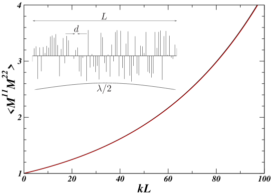
Figure 3: $\langle M^{11}M^{22}\rangle=\langle\alpha\alpha^{*}\rangle$ versus $kL$. Numerical results (bold line) from the one-dimensional model sketched in the inset are indistinguishable from the analytical results, Eq. (93). The results correspond to $x_{0}=2k\ell=200$ and $d/\ell=10^{-3}$.

The system of length $L$ is constructed from “delta potentials”, $U_{r}(x)=u_{r}\delta(x-x_{r})$ (recall that $U_{r}(x)$ and $u_{r}$ have dimensions of $k^{2}$ and $k$, respectively), located at the positions $x_{r}=rd$ ($r=0,1,2\dots$); $u_{r}$ is assumed to be uniformly distributed over the interval $[-u_{max},+u_{max}]$. The mean free path, obtained from Eq. (48), is simply given by:

$$\frac{d}{\ell}=\frac{1}{3}\left(\frac{u_{max}}{2k}\right)^{2}.$$ (94)

The results of the numerical calculations for $\langle\alpha\alpha^{*}\rangle$ and $\langle\alpha\beta\rangle$ versus $L$ are shown in Figs. 3 and 4, respectively. Averages were obtained from $10^{7}$ different microscopic realizations. Numerical results (bold line) are indistinguishable from the analytical solution of the diffusion equation (Eqs. (93) and (93b)).

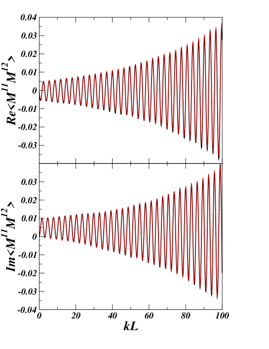
Figure 4: Real (top) and imaginary (bottom) parts of $\langle M^{11}M^{12}\rangle=\langle\alpha\beta\rangle$ as a function of $kL$. Numerical results (bold line) are indistinguishable from the analytical results. The parameters are the same as in Fig. 3.

It will be interesting to see what these results reduce to in the SWLA discussed in Sec. III.4 above. In preparation for this, we first consider a fixed value of $s=L/\ell$ and take $x_{0}=2k\ell\gg 1$. From Eq. (194) one can expand the functions $\left\langle\alpha\alpha^{\ast}\right\rangle_{s}$, $\left\langle\alpha\beta\right\rangle_{s}$ in powers of $1/x_{0}$; in terms of the original variables $k$, $\ell$ and $L$ they take the form

$$\left\langle\alpha\alpha^{\ast}\right\rangle_{s} = \frac{1}{2}(1+e^{2\frac{L}{\ell}})+\frac{2}{(2k\ell)^{2}}\left[-\left(1+2\frac{L}{\ell}\right)e^{2\frac{L}{\ell}}+e^{-\frac{L}{\ell}}\frac{e^{2ikL}+e^{-2ikL}}{2}\right]+O\left(\frac{1}{k\ell}\right)^{3}$$

$$\left\langle\alpha\beta\right\rangle_{s} = \frac{i}{2k\ell}\left(e^{-\frac{L}{\ell}}-e^{2\frac{L}{\ell}}e^{-2ikL}\right)+\frac{2}{(2k\ell)^{2}}\left[\frac{5-3\frac{L}{\ell}}{4}e^{-\frac{L}{\ell}}-\left(e^{2\frac{L}{\ell}}e^{-2ikL}+\frac{1}{4}e^{-\frac{L}{\ell}}e^{-4ikL}\right)\right]$$ (95b)

$$\hskip 170.71652pt+O\left(\frac{1}{k\ell}\right)^{3}\;.$$

The solutions (95) satisfy the differential equations (91) together with the initial conditions (92) to every order in the expansion in powers of $1/2k\ell$.

Notice that the ansatz made in Eq. (82) is verified explicitly in this example, with the result

$$\left\langle\alpha\alpha^{\ast}\right\rangle_{s}^{(0)} = \frac{1}{2}(1+e^{2\frac{L}{\ell}}),$$ (96a)

$$\left\langle\alpha\beta\right\rangle_{s}^{(0)} = 0,$$ (96b)

which represents, in this particular case, the SWLA discussed in Sec. III.4. The result (96a) agrees with what had been obtained earlier as a solution of the diffusion equation of Ref. mpk for $N=1$, also known as Melnikov’s equation. Notice that

$$\left\langle\beta\beta^{\ast}\right\rangle_{s}^{(0)}=\left\langle\alpha\alpha^{\ast}\right\rangle_{s}^{(0)}-1=\left\langle\frac{R}{T}\right\rangle_{s}^{(0)}=\frac{1}{2}(e^{2\frac{L}{\ell}}-1)$$ (97)

represents the well known exponential increase of Landauer’s resistance landauer .

If, in Eq. (95), we further expand the exponentials $e^{2L/\ell}$, $e^{-L/\ell}$, in powers of $1/\ell$, we end up with an expansion of $\left\langle\alpha\alpha^{\ast}\right\rangle_{s}$, $\left\langle\alpha\beta\right\rangle_{s}$ in powers of $1/\ell$. The result found in Eq. (61), setting $L=0$ and interpreting $\delta L$ as $L$, is precisely the term proportional to $1/\ell$ in such an expansion; we have verified the consistency of the two results up to $O(1/\ell)$.

IV.2 Random walk in the transfer matrix space: Numerical simulations.

As we have shown, the diffusion equation, Eq. (67), determines the statistical properties of transport for any physical observable and it only depends on the mean free paths $\ell_{ab}$. Once the various $\ell_{ab}$ are specified, the statistical distributions are universal, i.e., independent of other details of the microscopic statistics. However, in order to know the exact shape of the distribution of a given observable we have to solve the diffusion equation. This is a challenging problem even in the isotropic case mpk (where all the mfp’s are equivalent, $\ell_{ab}=\ell$). Here, instead of a direct solution of the multidimensional diffusion equation we have followed an alternative way that can be seen as a generalization of a random walk in the transfer matrix space (Ref. luis_thesis ). The method, based on our previous theoretical description, can be summarized as follows:

1) We first obtain a set of mean free paths from a given microscopic potential model for the building block or, eventually, from specific experiments on very thin slabs.

2) We generate an ensemble of transfer matrices having their first and second moments equal to those corresponding to a BB of a certain length $\delta L$.

3) The transfer matrix for a system of length $L=P\delta L$ is obtained by combining $P$ building block matrices randomly chosen from the ensemble. This procedure can be repeated again and again in order to obtain the statistical distribution of any physical quantity. As predicted by the CLT associated with the composition of BB’s explained in App. G, higher order moments of the BB matrix elements play no role in the final statistics.

The statistical distributions of different physical quantities will be shown to be in full agreement with the results of exact microscopic numerical calculations for a model system. This shows that validity of the diffusion equation given in Eq. (67) goes beyond the various formal limits discussed in Sec. III.

IV.2.1 Microscopic potential model and mean free paths

Let us consider the potential model sketched in Fig. 5.

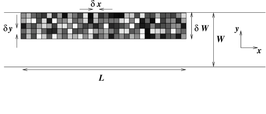
Figure 5: Schematic representation of the microscopic model based on random potentials. Each square of the plot, or “cell”, represents a region of constant random potential.

In this model, a 2D waveguide with perfectly reflecting walls has a region of length $L$ which is divided into small “cells” of dimensions $\delta x\times\delta y$. The working wavelength is chosen to be such that $\delta x,\delta y\ll\lambda$. In the language of Sec. III.1, the potential in the $r$-th slice, Eq. (21), is replaced here, for finite $\delta x$, by

$$U_{r}(x,y)=u_{r}(y)\frac{\theta_{\delta x}(x-x_{r})}{\delta x},$$ (98)

where $\theta_{\delta x}(x-x_{r})$ takes the value 1 inside the interval $(x_{r}-\delta x/2,\;x_{r}+\delta x/2)$ and 0 outside. Should $\delta x$ tend to zero, the expression in (98) would tend to that of Eq. (21a). Inside the $r$-th slice, the potential is taken to be constant within each cell, i.e.,

$$u_{r}(y)=\sum_{s}u_{s}\theta_{\delta y}(y-y_{r}),$$ (99)

so that

$$U_{r}(x,y)=\sum_{s}U_{s}\theta_{\delta x}(x-x_{r})\theta_{\delta y}(y-y_{r}),$$ (100)

with $U_{s}=u_{s}/\delta x$. The constant values $U_{s}$ of the potential inside each cell located in the region $W-\delta W<y<W$ is sampled from a uniform distribution within the interval $\left[-U_{0},U_{0}\right]$. Outside the region defined by $W-\delta W<y<W$, the potential is taken to be zero.

In order to get the mfp’s corresponding to our model system, we follow the same steps leading to Eq. (48) in Sec. III above. In the limit $\delta x,\delta y\ll\delta W$, and neglecting the coupling to evanescent modes, i.e., using the “bare” potential $u$ instead of the “effective” one $\hat{u}$ (see text following Eq. (28) and App. B), we obtain

$$\frac{1}{\ell_{ab}}=\frac{\langle\left[v_{ab}\right]^{2}\rangle}{\delta x}=\frac{U_{0}^{2}}{3}\frac{\delta x\delta y}{4k_{a}k_{b}}\int_{W-\delta W}^{W}\chi_{a}^{2}(y)\chi_{b}^{2}(y)dy,$$ (101)

where $\chi_{a}(y)$ are the transverse eigenfunctions of the clean waveguide (Eq. (15)). The mfp’s for bulk disordered systems, i.e., when the disordered potential covers the whole section of the waveguide ($\delta W=W$) are simply given by

$$\left.\frac{1}{\ell_{ab}}\right|_{\rm{bulk}}=\frac{U_{0}^{2}}{3}\frac{\delta x\delta y}{4k_{a}k_{b}}\frac{2+\delta_{ab}}{2W}.$$ (102)

In order to analyze a surface disordered waveguide, we shall also consider the limit $\delta W\ll W$,

$$\left.\frac{1}{\ell_{ab}}\right|_{\rm{surface}}=\frac{U_{0}^{2}}{3}\frac{\delta x\delta y}{4k_{a}k_{b}}\left(\frac{4\pi^{4}}{W^{2}}a^{2}b^{2}\delta W\right).$$ (103)

IV.2.2 Random transfer matrices for a building block

In order to generate an ensemble of random transfer matrices whose first and second moments are given, it is useful to describe the transfer matrix elements of the BB as a function of the $2N^{2}+N$ independent parameters of the Pereyra representation [see App. A, Eq. (130)]. The matrix $\varepsilon$ of Eq. (37d) can be expressed (in that representation) as

$$\varepsilon^{11} = e^{ih}\sqrt{1+\eta\eta^{\ast}}-1,$$ (104a)

$$\varepsilon^{12} = e^{ih}\eta,$$ (104b)

where $h$ is an arbitrary $N\times N$ Hermitian matrix (thus contributing $N^{2}$ parameters) and $\eta$ is an arbitrary $N\times N$ complex symmetric matrix (thus contributing $N^{2}+N$ parameters).

Applying successive approximations to Eqs. (104) it is possible to invert them to express the matrices $h$ and $\eta$ as functions of the blocks $\varepsilon^{ij}$, i.e.,

$$h = -i\varepsilon^{11}+\frac{i}{2}\left(\varepsilon^{12}\varepsilon^{21}+\varepsilon^{11}\varepsilon^{11}\right)+O\left(\varepsilon^{3}\right),$$ (105a)

$$\eta = \varepsilon^{12}-\varepsilon^{11}\varepsilon^{12}+O\left(\varepsilon^{3}\right).$$ (105b)

The aim is to derive the statistical properties of the matrices $h$ and $\eta$ in terms of those of the blocks $\varepsilon^{ij}$ which we derived in the previous section; we shall do this in the SWLA (see Sec. III.4). We can use Eqs. (105), (80) and (81) to obtain (in powers of $\delta L$) the first and second moments of the matrix elements $\eta_{ab}$, $h_{ab}$. For the first moments we obtain

$$\left\langle h_{ab}\right\rangle_{\delta L} = O\left(\delta L\right)^{2},$$ (106a)

$$\left\langle\eta_{ab}\right\rangle_{\delta L} = O\left(\delta L\right)^{2},$$ (106b)

and for the second moments

$$\left\langle h_{ab}h_{cd}\right\rangle_{\delta L} = -\left\langle\varepsilon_{ab}^{11}\varepsilon_{cd}^{11}\right\rangle_{\delta L}+\cdots=\frac{\delta L}{1+\delta_{ac}}\left[\delta_{ab}\delta_{cd}\frac{C\left(aa,cc\right)}{\sqrt{\ell_{aa}\ell_{cc}}}+\frac{\delta_{ad}\delta_{bc}}{\ell_{ab}}\right]$$

$$+O\left(\delta L\right)^{2},$$

$$\left\langle h_{ab}h_{cd}^{\ast}\right\rangle_{\delta L} = -\left\langle\varepsilon_{ab}^{11}\varepsilon_{cd}^{22}\right\rangle_{\delta L}+\cdots=\frac{\delta L}{1+\delta_{ad}}\left[\delta_{ab}\delta_{cd}\frac{C\left(aa,cc\right)}{\sqrt{\ell_{aa}\ell_{cc}}}+\frac{\delta_{ac}\delta_{bd}}{\ell_{ab}}\right]$$

$$+O\left(\delta L\right)^{2},$$

$$\left\langle h_{ab}\eta_{cd}\right\rangle_{\delta L} = -i\left\langle\varepsilon_{ab}^{11}\varepsilon_{cd}^{12}\right\rangle_{\delta L}+\cdots=O\left(\delta L\right)^{2},$$ (107c)

$$\left\langle h_{ab}\eta_{cd}^{\ast}\right\rangle_{\delta L} = -i\left\langle\varepsilon_{ab}^{11}\varepsilon_{cd}^{21}\right\rangle_{\delta L}+\cdots=O\left(\delta L\right)^{2},$$ (107d)

$$\left\langle\eta_{ab}\eta_{cd}\right\rangle_{\delta L} = \left\langle\varepsilon_{ab}^{12}\varepsilon_{cd}^{12}\right\rangle_{\delta L}+\cdots=O\left(\delta L\right)^{2},$$ (107e)

$$\left\langle\eta_{ab}\eta_{cd}^{\ast}\right\rangle_{\delta L} = \left\langle\varepsilon_{ab}^{12}\varepsilon_{cd}^{21}\right\rangle_{\delta L}+\cdots=\frac{\delta_{ac}\delta_{bd}+\delta_{ad}\delta_{bc}}{1+\delta_{ab}}\frac{\delta L}{\ell_{ab}}+O\left(\delta L\right)^{2}.$$ (107f)

To generate the ensemble of random transfer matrices for $\eta$ and $h$ in the SWLA, we need to know the statistical properties of the real and imaginary parts of the matrix elements $\eta_{ab}$ and $h_{ab}$, to be denoted as

$$\eta_{ab}^{R} \equiv \textrm{Re}\eta_{ab}=\frac{1}{2}\left(\eta_{ab}+\eta_{ab}^{\ast}\right),\qquad\eta_{ab}^{I}\equiv\textrm{Im}\eta_{ab}=\frac{1}{2i}\left(\eta_{ab}-\eta_{ab}^{\ast}\right),$$ (108a)

$$h_{ab}^{R} \equiv \textrm{Re}h_{ab}=\frac{1}{2}\left(h_{ab}+h_{ab}^{\ast}\right),\qquad h_{ab}^{I}\equiv\textrm{Im}h_{ab}=\frac{1}{2i}\left(h_{ab}-h_{ab}^{\ast}\right).$$ (108b)

Using Eqs. (106) and (107) we find

$$\left\langle\left(\eta_{ab}^{R}\right)^{2}\right\rangle_{\delta L} = \left\langle\left(\eta_{ab}^{I}\right)^{2}\right\rangle_{\delta L}=\frac{\delta L}{2\ell_{ab}}+O\left(\delta L\right)^{2},\;\hskip 14.22636pt\forall a,b,$$ (109a)

$$\left\langle\left(h_{ab}^{R}\right)^{2}\right\rangle_{\delta L} = \left\langle\left(h_{ab}^{I}\right)^{2}\right\rangle_{\delta L}=\frac{\delta L}{2\ell_{ab}}+O\left(\delta L\right)^{2},\hskip 14.22636pta\neq b,$$ (109b)

$$\left\langle\left(h_{aa}\right)^{2}\right\rangle_{\delta L} = \frac{\delta L}{\ell_{aa}}+O\left(\delta L\right)^{2},$$ (109c)

$$\left\langle h_{aa}h_{bb}\right\rangle_{\delta L} = \frac{C\left(aa,bb\right)}{\sqrt{\ell_{aa}\ell_{bb}}}\delta L+O\left(\delta L\right)^{2},$$ (109d)

$$\left\langle h_{ab}^{R}h_{cd}^{R}\right\rangle_{\delta L} = \left\langle h_{ab}^{I}h_{cd}^{I}\right\rangle_{\delta L}=\left\langle h_{ab}^{R}h_{cd}^{I}\right\rangle_{\delta L}=O\left(\delta L\right)^{2},\hskip 14.22636pta\neq b\neq c\neq d,$$ (109e)

$$\left\langle h_{ab}^{R}h_{ad}^{R}\right\rangle_{\delta L} = \left\langle h_{ab}^{I}h_{ad}^{I}\right\rangle_{\delta L}=\left\langle h_{ab}^{R}h_{ad}^{I}\right\rangle_{\delta L}=O\left(\delta L\right)^{2},\hskip 14.22636pta\neq b\neq d,$$ (109f)

$$\left\langle h_{ab}^{R}\eta_{cd}^{R}\right\rangle_{\delta L} = \left\langle h_{ab}^{I}\eta_{cd}^{I}\right\rangle_{\delta L}=\left\langle h_{ab}^{R}\eta_{cd}^{I}\right\rangle_{\delta L}=\left\langle h_{ab}^{I}\eta_{cd}^{R}\right\rangle_{\delta L}=O\left(\delta L\right)^{2},$$ (109g)

$$\left\langle\eta_{ab}^{R}\eta_{cd}^{I}\right\rangle_{\delta L} = \left\langle h_{ab}^{R}h_{cd}^{I}\right\rangle_{\delta L}=O\left(\delta L\right)^{2}$$ (109h)

$$\left\langle\eta_{ab}^{R}\eta_{cd}^{R}\right\rangle_{\delta L} = \left\langle\eta_{ab}^{I}\eta_{cd}^{I}\right\rangle_{\delta L}=O\left(\delta L\right)^{2},\hskip 14.22636pta\neq c,\;b\neq d,$$ (109i)

$$\left\langle\eta_{ab}^{R}\eta_{ad}^{R}\right\rangle_{\delta L} = \left\langle\eta_{ab}^{I}\eta_{ad}^{I}\right\rangle_{\delta L}=\left\langle\eta_{ab}^{R}\eta_{ad}^{I}\right\rangle_{\delta L}=O\left(\delta L\right)^{2},\hskip 14.22636pta\neq b\neq d.$$ (109j)

We recall that the diagonal elements $h_{aa}$ are real since $h$ is a Hermitian matrix.

From now on, to generate the ensemble we shall consider a potential which is delta correlated in the transverse direction; in that case we have

$$\frac{C\left(aa,bb\right)}{\sqrt{\ell_{aa}\ell_{bb}}}=\frac{1}{\ell_{ab}},$$ (110)

which allows rewriting Eqs. (109c)-(109d) as one equation:

$$\left\langle h_{aa}h_{bb}\right\rangle_{\delta L}=\frac{\delta L}{\ell_{ab}}+O\left(\delta L\right)^{2}.$$ (111)

Therefore, in the SWLA, real and imaginary parts of the matrix elements of $\eta$ and off-diagonal matrix elements of $h$ are, to order $\delta L$, uncorrelated, with zero mean, Eq. (106), and with variance $\delta L/2\ell_{ab}$, Eqs. (109a) and (109b). For these elements we have used two different distributions giving the same variances:

$$P_{1}\left(x\right) = \frac{1}{4\sqrt{3}\sigma}\left[\theta\left(x+\sqrt{3}\sigma\right)-\theta\left(x-\sqrt{3}\sigma\right)\right],$$ (112a)

$$P_{2}\left(x\right) = \frac{1}{2}\delta\left(x-\sigma\right)+\frac{1}{2}\delta\left(x+\sigma\right),$$ (112b)

$\theta\left(x\right)$ being the usual step function and $\sigma^{2}=\mathrm{var}\left(x\right)$. As we can see from the CLT of App. G, the final results only depend on the coefficients proportional to $\delta L$, while the rest of the details of the distributions do not play any role.

In contrast, the diagonal elements of the $h$ matrices are correlated, Eq. (111). In order to generate numerically a set of uncorrelated variables from the diagonal elements of the $h$ matrices we have performed an orthogonal transformation on the diagonal terms $h_{aa}$,

$$h_{aa}^{\prime}=\sum_{b}O_{ab}h_{bb},$$ (113)

in such a way that the covariance matrix $C_{ab}\equiv\left\langle h_{aa}h_{bb}\right\rangle=\delta L/\ell_{ab}$ is diagonalized, to obtain

$$\left\langle h^{\prime}_{aa}h^{\prime}_{bb}\right\rangle=\delta_{ab}\sigma_{a}^{2}.$$ (114)

Hence we can numerically generate a set of $N$ uncorrelated variables $h^{\prime}_{aa}$ with zero mean and a variance given by the eigenvalues of the $C_{ab}=\delta L/\ell_{ab}$ matrix and, after that, obtain, by the change of coordinates (113), the $h_{aa}$ variables which are properly correlated.

IV.2.3 Random walk in the transfer-matrix space: Statistical conductance distributions

Once we have numerically generated an ensemble of transfer matrices with its first and second moments correct up to order $\delta L$, we can obtain a transfer matrix corresponding to a system of length $L=P\delta L$ by multiplying $P$ transfer matrices of the ensemble of BB’s taken at random. Numerically this procedure is unstable because the pseudounitary group, to which the transfer matrices belong, is non-compact mello-kumar . This property leads to numerical instabilities as the norm of the transfer matrix elements can grow without limit. Instead of using the product of transfer matrices, we obtain the scattering matrix associated with each transfer matrix (Eqs. (124)), and then combine different scattering matrices to obtain the scattering matrix for the system of length $L$ (Eqs. (132)).

For a given set of mean free paths $\ell_{ab}$ we choose the length $\delta L$ of the BB in such a way that $\delta L/\ell_{ab}\ll 1$ for all channels. With this, we generate random transfer matrices as explained above and, for each one, we obtain the corresponding scattering matrix. Applying Eq. (132) $P$ times we obtain the scattering matrix corresponding to a system of length $L=P\delta L$. This procedure can be repeated as many times as needed to obtain the desired statistical properties.

A detailed numerical analysis of the statistical properties is beyond the scope of the present work and will be discussed elsewhere. Here we just focus on the statistical distribution of the conductance and the intriguing discrepancies between surface and bulk disordered systems UAM ; UAM2 .

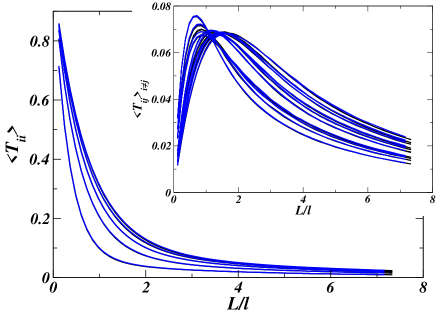
Figure 6: Bulk disordered waveguides: Average transmittances $\left\langle T_{ii}\right\rangle$ (channel in = channel out), as a function of $L/\ell$. The inset shows the equivalent results for $\left\langle T_{ij}\right\rangle$ with $i\neq j$. The results based on the numerical solution of the Schródinger equation (microscopic calculation) and the random walk simulation of the diffusion equation in the SWLA overlap.

Bulk Disorder

The behavior of the average transmittances $\left\langle T_{ii}\right\rangle$ (channel in = channel out), for bulk disordered wires, is plotted in Fig. 6 as a function of $L/\ell$, $\ell$ being the averaged transport mean free path,

$$\frac{1}{\ell}\equiv\frac{1}{N}\sum_{ab}\frac{1}{\ell_{ab}}.$$ (115)

The inset shows the equivalent results for $\left\langle T_{ij}\right\rangle$ with $i\neq j$. The random-walk simulation was performed in the SWLA. We have also solved numerically the Schrödinger equation for the same model system (sketched in Fig. 5). We followed an implementation of the so-called generalized scattering matrix (GSM) method (see for example Ref. JJS_evanesc ). The first step consists in the calculation of the set of transverse eigenfunctions and the scattering matrix for each slice of length $\delta x$. The combination of two consecutive slices is done by mode matching at the interface. After that we combine scattering matrices to obtain the scattering matrix of the whole system. It is important to mention that this calculation is performed using both propagating and evanescent modes and hence, this method can be considered as exact. The statistical properties of any transport parameter obtained from $10^{5}$ different realizations were found to converge for 3 evanescent modes. The calculations have been done starting from the set of mean free paths $\ell_{ab}$ given by Eq. (102) for $kW=5.5\pi$ (corresponding to 5 propagating modes), $U_{0}W^{2}=100$ and $\delta x/W=\delta y/W=1/50$. The exact numerical results for the average transmission coefficients are indistinguishable from the random-walk simulations.

The random-walk results for the average reflection coefficients $\left\langle R_{ij}\right\rangle$ for bulk disorder (shown in Fig. 7) are also in good agreement with our numerical results as well as with previous numerical work PGM (using a two-dimensional Tight-Binding model with Anderson disorder). The set of reflection coefficients corresponding to backscattering ($\left\langle R_{ii}\right\rangle$) are consistent with an enhanced backscattering factor $\left\langle R_{ii}\right\rangle/\left\langle R_{ij}\right\rangle\approx 2$, as expected from the DMPK equation.

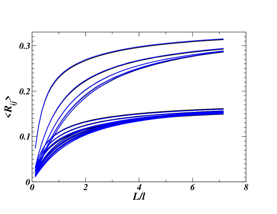
Figure 7: Bulk disordered waveguides: Average reflectance $\left\langle R_{ij}\right\rangle$ as a function of $L/\ell$. The upper curves correspond to $i=j$ and the lower curves to $i\neq j$. The results based on the numerical solution of the Schródinger equation (microscopic calculation) and the random walk simulation of the diffusion equation in the SWLA overlap.

The distribution of the dimensionless conductance, $P(g)$ [with $g=\text{trace}(tt^{\dagger})$], for bulk disordered wires is plotted in Fig. 8 for different conductance averages, $\langle g\rangle$. The inset shows the average conductance as a function of $L/\ell$.

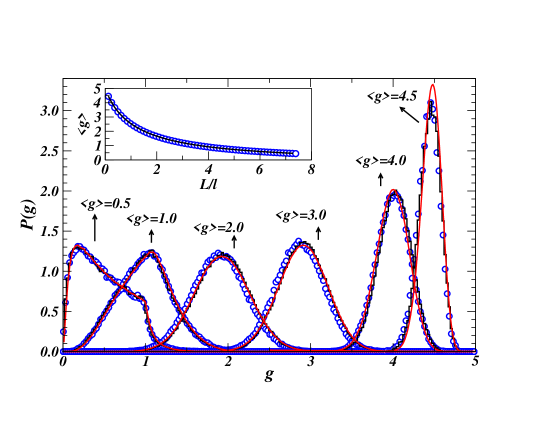
Figure 8: Bulk disordered waveguides: Distribution of the dimensionless conductance, $P(g)$, for different conductance averages, $\langle g\rangle$. The three different curves based on different approaches overlap. Circles correspond to the random walk simulation of the diffusion equation in the SWLA. The continuous line represents the results of the Montecarlo simulation of Ref. UAM . The histogram lines are the results based on the numerical solution of the Schrödinger equation (microscopic calculation). The inset shows the average conductance as a function of $L/\ell$.

The exact numerical results for the conductance distribution (histogram lines in Fig. 8) are indistinguishable from the random walk simulations (open circles). For comparison we also plot (continuous line) the exact result of the diffusion equation of Ref. mpk (DMPK equation) obtained from a Montecarlo simulation UAM . Despite the slight channel anisotropy of transport, the results are compatible with those of the DMPK equation.

Surface Disorder

In the case of surface disorder, the mean free paths are very different from those obtained for a uniform (bulk) distribution of scatterers. In particular, the dependence of $\ell_{ab}$ on $a^{2}b^{2}$ [see Eq. (103)] reflects the strong channel anisotropy of transport in surface disordered waveguides WRM ; AGM_apl ; freilikher ; izrailev_1 ; izrailev_2 ; rendon . This could be the origin of the differences between bulk and surface distributions. Previous numerical calculations for surface disordered waveguides, showed that close to the onset of localization, the conductance distributions presented an unexpected sharp cusp-like shape UAM2 . The distribution of the dimensionless conductance for surface disordered wires obtained from the random walk simulation in the SWLA is plotted in Fig. 9 (open circles) for different conductance averages. The exact solution of the Schrödinger equation (microscopic calculation; histograms) is again in full agreement with the diffusion equation and with previous numerical work WRM ; UAM2 . The calculations have been done starting from the set of mean free paths $\ell_{ab}$ given by Eq. (103) for $\delta W=0.1W$, $U_{0}=100/W^{2}$, $kW=5.5\pi$ ($N=5$), $\delta x=10\delta y=W/50$.

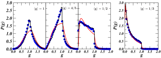
Figure 9: Surface disordered waveguides: Distribution of the dimensionless conductance, $P(g)$, for different conductance averages, $\langle g\rangle$. Circles correspond to the random walk simulation of the diffusion equation in the SWLA. The histogram lines are the results based on the numerical solution of the Schrödinger equation (microscopic calculation). The equivalent results for bulk disorder (continuous line, DMPK) are also shown for comparison.

It is worth noticing that when the disordered region is confined close to the surface, the mean free paths can be extremely large (for example, for the present calculation, $\ell\approx 1.50\times 10^{4}W$). The exact numerical solution of the wave equation is then extremely expensive in terms of computation time compared to the random walk simulations based on the statistical properties of the BB.

Although the random walk in the SWLA accurately reproduces the exact conductance distributions, it is not in full agreement with the statistical properties of the different transmittances. As an example, Fig. 10 shows the behavior of $\langle T_{a}\rangle=\sum_{b}\langle T_{ba}\rangle$ versus $L/\ell$ for both the exact numerical results (continuous lines) and the random walk (dashed lines). The disagreement could be associated to the use of an approximate expression (Eq. (103)) for the mean free paths. For small lengths compared to the mean free paths, the average reflectance is given by (see also Eq. (46))

$$\left\langle R_{ab}\right\rangle=\frac{L}{\ell_{ab}}+\cdots.$$ (116)

We could then have obtained the different mean free paths $\ell_{ab}$ for all modes by performing a linear fitting of the numerical results to Eq. (116). However, as long as the energy is not very close to the onset of new propagating channels, we found that the numerical mfp’s are well described by Eqs. (102) and (103) within the numerical accuracy. The discrepancy could then be associated to the limitations of the SWLA. The generalization of the random walk method beyond the SWLA is in progress.

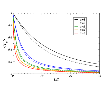
Figure 10: Surface disordered waveguides: Average transmittances $\left\langle T_{a}\right\rangle$ as a function of $L/\ell$. The agreement between results based on the numerical solution of the Schrödinger equation (microscopic calculation; continuous lines) and the random walk simulation of the diffusion equation in the SWLA (dashed lines) is not as good as for the conductance distributions.

In summary, we have implemented a numerical method to obtain the statistical properties of the transport coefficients using the diffusion equation derived in this work. We have extensive numerical evidence of the suitability of our model to describe the statistics of wave transport in disordered waveguides. It is worth noticing that our model exactly reproduces the conductance distributions obtained from the microscopic model even though this one contains as many evanescent modes as needed to perform the calculation in an exact manner. The only parameters needed to obtain the statistics of any transport coefficient are the mean free paths $\ell_{ab}$, as it is implied by the diffusion equation, all the statistical properties being fixed at any length once all $\ell_{ab}$ parameters are fixed.

V Conclusions and Discussion

The central result of the present paper is the Fokker-Planck equation, Eq. (12), which describes the evolution with the length $L$ of a disordered waveguide of transport properties which can be expressed in terms of the transfer matrix $\bm{M}$ of the system.

Our starting point is a potential model in which the scattering units consist of thin potential slices (taken as delta slices for convenience) perpendicular to the longitudinal direction of the waveguide, the variation of the potential in the transverse direction being arbitrary. A statistical law for the potential slices is specified, as detailed in Sec. III.2.1: in particular, the parameters of a given slice are taken to be statistically independent from those of any other slice, so that we are dealing here with the situation of uncorrelated (at least in the longitudinal direction) disorder. Our result is obtained in the so called dense-weak-scattering limit, denoted by DWSL in the text, in which each potential slice is very weak and the linear density of slices is very large, so that the resulting mean free paths (mfp’s) are fixed (see Eq. (50d)). The statistical properties of a building block (denoted by BB) of length $\delta L$, say, are first derived; the BB is then added to a waveguide of length $L$ to obtain a composition law, from which the diffusion equation is eventually derived. In the DWSL, the statistical properties of the BB, and hence of the full system, depend only on the mfp’s which, in turn, depend only on the second moments of the individual delta-potential strengths. Cumulants of the potential higher than the second are irrelevant in the limit, signalling the existence of a generalized central-limit theorem (CLT): once the mfp’s are specified, the limiting equation (12) is universal, i.e., independent of other details of the microscopic statistics.

One important characteristic of the present analysis, compared with previous ones, is that the energy of the incident particle is fully taken into account, a consequence being that the generalized diffusion coefficients appearing in the diffusion equation (12) depend on the wavenumber $k$ of the incident wave and on the length $L$.

The diffusion equation (12) for expectation values is very difficult to solve, the main reason being explained in the text, right below Eq. (92). The original DMPK equation mpk for the probability distribution of certain parameters of the transfer matrix was solved exactly for the unitary symmetry class only beenakker_rejaei , whereas for the evolution of expectation values arising from that same equation for a large number of open channels, $N\gg 1$, an iterative procedure was developed to find the result as an expansion in powers of $1/N$ mello-kumar . In the present case, in Sec. IV.1 we have been able to solve Eq. (12) exactly for $N=1$, but only for a few particular observables: the solution is in excellent agreement with the results of a microscopic calculation. However, not even for $N\gg 1$ have we been able to develop an analytic iterative procedure like the one we mentioned above; even numerically we have not succeeded in developing a method to solve Eq. (12). We have thus tackled the problem of extracting information from the analysis of the present paper from a different point of view, based on the study of the BB itself, which was shown to have universal statistical properties. First, we should remark that the BB is useful not only as an intermediate step to obtain the diffusion equation; it is interesting as a physical system in itself, i.e., a slab. In the paper we obtained its statistical properties up to order $\delta L$ only, with some extension to order $(\delta L)^{2}$. In principle, although it represents a tedious task, the procedure could be carried on to at least a few more powers of $\delta L$. A similar expansion was performed in an earlier publication mello_tomsovic . Second, the BB was used in Sec. IV.2 to develop the method that we called “random walk in the transfer matrix space”, which was essential for the numerical analysis based on the results of the present work. The results reported in that section showed excellent agreement with the corresponding microscopic calculations. Efforts towards an analytical and/or numerical treatment of the diffusion equation (12) itself would be very important.

In Sec. III.4 we develop the short-wavelength approximation, denoted as SWLA in the text, which bears resemblance to the geometrical optics limit studied in optics. The results of this approximation allow making a connection with some of our previous work, in which the energy did not appear explicitly in the analysis. We should remark that the numerical results of the random walk in the transfer matrix space reported in Sec. IV.2 were performed within this approximation.

In the analysis presented in this paper, the presence of evanescent modes for a single slice appears in the effective potential $(\hat{u}_{r})_{ab}$ that occurs in Eq. (28) and is used to construct the open-channel transfer matrix; the effective potential takes into account transitions to evanescent modes. Our statistical law is thus postulated for the matrix elements of the effective potential. However, as we mentioned in Sec. II around Eq. (4) and in Sec. IV.2.3, the transfer matrix for a sequence of scatterers was constructed multiplying open-channel transfer matrices, i.e., ignoring the presence of evanescent modes in the combination law. Nonetheless, the final agreement with microscopic calculations is very good. An important question for future investigation is thus to understand the effect of evanescent modes when combining subsystems to form the whole waveguide.

In the potential model developed here the property of time-reversal invariance is satisfied and the treatment is also restricted to scalar waves. In the language of random-matrix theory, we are dealing with the orthogonal symmetry class, or $\beta=1$. For possible applications to electronic systems, it would be interesting to extend the analysis to the unitary and symplectic cases, $\beta=2$ and $\beta=4$, respectively.

As explained in the Introduction, in earlier publications (like Refs. mpk ; mello-kumar ) the notion of maximum entropy in conjunction with a number of physical constraints played an important role in selecting the distribution of the BB: in a way, that selection captured the features arising from a CLT. We think that it would be very interesting to investigate the question whether the results presented here can be obtained within such a framework.

Finally, since the results of our model have been compared successfully only with microscopic computer simulations, we think that it would be very challenging to measure these same quantities in the laboratory, in order to make comparisons with real-life experiments.

Appendix A Some Properties of the Transfer Matrix

A.1 Transfer and Scattering Matrices

The transfer matrix $\bm{M}$ is closely related to a perhaps more familiar object: the scattering or $\bm{S}$ matrix, that relates incoming to outgoing waves:

$$\bm{S}=\left(\begin{array}[]{cc}r&t^{\prime}\\ t&r^{\prime}\end{array}\right).$$ (117)

The $N$-dimensional blocks of the $\bm{M}$ matrix (Eq. (3)),

$$\bm{M}=\left[\begin{array}[]{ll}M^{11}&M^{12}\\ M^{21}&M^{22}\end{array}\right]\equiv\left[\begin{array}[]{ll}\alpha&\beta\\ \gamma&\delta\end{array}\right],$$ (118)

are related to the reflection and transmission matrices $r,t$ for left incidence and $r^{\prime},t^{\prime}$ for right incidence as

$$r = -\delta^{-1}\gamma,\hskip 28.45274ptt^{\prime}=\delta^{-1}$$ (119a)

$$t = (\alpha^{\dagger})^{-1},\hskip 28.45274ptr^{\prime}=\beta\delta^{-1}.$$ (119b)

The physical property of flux conservation (FC) requires the $\bm{S}$ matrix to be unitary ($\bm{S}\bm{S}^{\dagger}=\bm{1}$) while the $\bm{M}$ matrix must satisfy the pseudounitarity condition

$$\bm{M}^{\dagger}\bm{\Sigma}_{z}\bm{M}=\bm{\Sigma}_{z}.$$ (120)

This is the only condition that $\bm{M}$ satisfies in the unitary, or $\beta=2$, case. If, in addition, the system is time-reversal invariant (TRI), i.e., in the orthogonal case $\beta=1$, we have the extra condition

$$\bm{M}^{*}=\bm{\Sigma}_{x}\bm{M}\bm{\Sigma}_{x},$$ (121)

where $\bm{\Sigma}_{z}$ and $\bm{\Sigma}_{x}$ have the structure of Pauli matrices:

$$\bm{\Sigma}_{z}=\left(\begin{array}[]{cc}1&0\\ 0&-1\end{array}\right)\quad,\quad\bm{\Sigma}_{x}=\left(\begin{array}[]{cc}0&1\\ 1&0\end{array}\right).$$ (122)

Eq. (121) implies

$$M^{22}=\left(M^{11}\right)^{*},\qquad M^{21}=\left(M^{12}\right)^{*},$$ (123)

so that in Eq. (3) only the two blocks $M^{11}$ and $M^{12}$, or $\alpha$ and $\beta$, need be considered. The relation with the reflection and transmission matrices in the TRI case is now

$$r = -(\alpha^{\ast})^{-1}\beta^{\ast},\hskip 28.45274ptt^{\prime}=(\alpha^{\ast})^{-1}$$ (124a)

$$t = (\alpha^{\dagger})^{-1},\hskip 28.45274pt\;\;\;\;\;\;r^{\prime}=\beta(\alpha^{\ast})^{-1}.$$ (124b)

In this TRI case, the matrix $\bm{\varepsilon}$ for the BB, defined in Eq. (6), must satisfy the relations

$$\bm{\varepsilon}^{*}=\bm{\Sigma}_{x}\bm{\varepsilon}\Sigma_{x},$$ (125)

so that

$$\varepsilon^{21} = (\varepsilon^{12})^{*}$$ (126a)

$$\varepsilon^{22} = (\varepsilon^{11})^{*}.$$ (126b)

Introducing the notation

$$\overline{1}=2,\qquad\overline{2}=1,$$ (127)

the TRI relations (126) can be written as

$$\epsilon_{ab}^{\bar{i}\;\bar{j}}=(\epsilon_{ab}^{ij})^{*}.$$ (128)

A.2 The transfer matrix in terms of independent parameters

FC and TRI symmetry imply that the actual number of independent parameters of a transfer matrix is $2N^{2}+N$. This fact can be taken explicity into account by writing $\bm{M}$ in a polar representation as mello-kumar

$$\bm{M}=\left[\begin{array}[]{cc}\bm{u}&0\\ 0&\bm{u}^{*}\end{array}\right]\left[\begin{array}[]{cc}\sqrt{1+\lambda}&\sqrt{\lambda}\\ \sqrt{\lambda}&\sqrt{1+\lambda}\end{array}\right]\left[\begin{array}[]{cc}\bm{v}&0\\ 0&\bm{v}^{*}\end{array}\right],$$ (129)

where $\bm{u},\bm{v}$ are arbitrary $N\times N$ unitary matrices (each contributing $N^{2}$ parameters) and $\bm{\lambda}$ is a real diagonal matrix with $N$ arbitrary non-negative elements.

Another useful representation was introduced by Pereyra pereyra

$$\bm{M}=\left[\begin{array}[]{cc}e^{ih}&0\\ 0&e^{-ih^{*}}\end{array}\right]\left[\begin{array}[]{cc}\sqrt{1+\eta\eta^{*}}&\eta\\ \eta^{*}&\sqrt{1+\eta^{*}\eta}\end{array}\right],$$ (130)

where $h$ is an arbitrary $N\times N$ Hermitian matrix (thus contributing $N^{2}$ parameters) and $\eta$ is an arbitrary $N\times N$ complex symmetric matrix (with $N^{2}+N$ parameters).

A.3 Multiplicativity property

Suppose we start with a system having a transfer matrix $\bm{M}_{1}$ and enlarge it by adding, on its right hand side, another system having a transfer matrix $\bm{M}_{2}$; the transfer matrix of the combined system is simply given by

$$\bm{M}=\bm{M}_{2}\bm{M}_{1}.$$ (131)

The role of closed channels (evanescent modes) is briefly discussed in the text, around Eq. (4). This multiplicativity property is extremely useful and is extensively used in the analytic study along the present work. However, from a numerical point of view, the successive multiplication of $\bm{M}$-matrices is unstable because the pseudounitary group, to which the transfer matrices belong, is not compact mello-kumar . This property leads to numerical instabilities as the norm of the transfer matrix elements can grow without limit. In contrast, numerical methods based on the scattering matrix can be very effective and stable JJS_evanesc : if we have the scattering matrices $\bm{S}_{1}$ and $\bm{S}_{2}$, the scattering matrix $\bm{S}$ corresponding to the composition of the subsystems $(1)$ on the left and $(2)$ on the right is given by

$$r = r_{1}+t^{\prime}_{1}r_{2}Qt_{1}$$ (132a)

$$t = t_{2}Qt_{1}$$ (132b)

$$t^{\prime} = (t)^{\top}$$ (132c)

$$r^{\prime} = t_{2}Qr^{\prime}_{1}t^{\prime}_{2}+r_{2}$$ (132d)

where

$$Q\equiv\left(\bm{I}_{N}-r^{\prime}_{1}r_{2}\right)^{-1}$$ (133)

and $\bm{I}_{N}$ denotes the $N\times N$ unit matrix.

Appendix B Evanescent Modes and the Effective Potential

In this appendix we define the effective potential for a delta slice that was introduced in Eqs. (26) and (28).

Consider a problem admitting $N$ open channels and $N^{\prime}$ closed ones. We shall eventually be interested in the limit $N^{\prime}\to\infty$. The total number of channels will be denoted by $N_{T}=N+N^{\prime}$. It will be convenient to define projection operators $P$ and $Q$ (with $P+Q=I$) unto open and closed channels, respectively, i.e.,

$$P = \sum_{a=1}^{N}\left|\chi_{a}\right\rangle\left\langle\chi_{a}\right|,$$ (134a)

$$Q = \sum_{a=N+1}^{N_{T}}\left|\chi_{a}\right\rangle\left\langle\chi_{a}\right|,$$ (134b)

where $\left|\chi_{a}\right\rangle$ represents the “transverse” state defined in Eq. (15). The most general solution of the Schrödinger equation on either side of the scattering system contains:

i) incoming- and outgoing-wave amplitudes for all the open channels. We denote by $\tilde{a}_{P}^{(1)}$, $\tilde{a}_{P}^{(2)}$ the $N$-component vectors of incoming open-channel amplitudes on the left and right of the system, respectively, while $\tilde{b}_{P}^{(1)}$, $\tilde{b}_{P}^{(2)}$ denote the corresponding outgoing open-channel amplitudes.

ii) “outgoing” closed-channel amplitudes, denoted by the $N^{\prime}$-component vectors $\tilde{b}_{Q}^{(1)}$, $\tilde{b}_{Q}^{(2)}$, on the left and right of the system, respectively: these are the components that decrease exponentially at infinity. The $N^{\prime}$-component vectors $\tilde{a}_{Q}^{(1)}$, $\tilde{a}_{Q}^{(2)}$ represent the “incoming” closed-channel amplitudes, i.e., the components that increase exponentially at infinity. In order to have a normalizable (in the Dirac delta-function sense) wave function, closed channels can only give an exponentially vanishing contribution at infinity, so that the components $\tilde{a}_{Q}^{(1)}$, $\tilde{a}_{Q}^{(2)}$, which we keep for convenience in the following equation, will eventually be set equal to zero. We shall also use the notation $\widetilde{\alpha}_{PP}\equiv P\alpha P$, etc. The wave amplitudes on the two sides are then related by the “extended transfer matrix” mello-kumar as follows:

$$\left[\begin{tabular}[]{c}\begin{tabular}[]{c}$\widetilde{b}_{P}^{(2)}$\\ $\widetilde{b}_{Q}^{(2)}$\end{tabular}\\ \hline\cr\begin{tabular}[]{c}$\widetilde{a}_{P}^{(2)}$\\ $\widetilde{a}_{Q}^{(2)}$\end{tabular}\end{tabular}\right]=\left[\begin{tabular}[]{c|c}\begin{tabular}[]{cc}$\widetilde{\alpha}_{PP}$&$\widetilde{\alpha}_{PQ}$\\ $\widetilde{\alpha}_{QP}$&$\widetilde{\alpha}_{QQ}$\end{tabular}&\begin{tabular}[]{cc}$\widetilde{\beta}_{PP}$&$\widetilde{\beta}_{PQ}$\\ $\widetilde{\beta}_{QP}$&$\widetilde{\beta}_{QQ}$\end{tabular}\\ \hline\cr\begin{tabular}[]{cc}$\widetilde{\gamma}_{PP}$&$\widetilde{\gamma}_{PQ}$\\ $\widetilde{\gamma}_{QP}$&$\widetilde{\gamma}_{QQ}$\end{tabular}&\begin{tabular}[]{cc}$\widetilde{\delta}_{PP}$&$\widetilde{\delta}_{PQ}$\\ $\widetilde{\delta}_{QP}$&$\widetilde{\delta}_{QQ}$\end{tabular}\end{tabular}\right]\left[\begin{tabular}[]{c}\begin{tabular}[]{c}$\widetilde{a}_{P}^{(1)}$\\ $\widetilde{a}_{Q}^{(1)}$\end{tabular}\\ \hline\cr\begin{tabular}[]{c}$\widetilde{b}_{P}^{(1)}$\\ $\widetilde{b}_{Q}^{(1)}$\end{tabular}\end{tabular}\right]\;.$$ (135)

Here we are using the notation of Ref. mello-kumar , which was developed in terms of incoming- and outgoing- wave amplitudes, both for the $S$ matrix and for the $M$ matrix. This results in an asymmetry in the notation in the two vectors appearing in Eq. (135). Perhaps a more common notation expresses the $M$ matrix in terms of waves that travel to the right and to the left, giving a more symmetric definition.

The extended transfer matrix of Eq. (135), which will be denoted by $\tilde{M}$, contains four $N_{T}\times N_{T}$ matrix blocks. When we set, as we already mentioned, the amplitudes ${a}_{Q}^{(1)}={a}_{Q}^{(2)}=0$ and consider, as given data, the $2N$ amplitudes ${a}_{P}^{(1)}$, ${b}_{P}^{(1)}$, we obtain a set of $2(N+N^{\prime})$ equations in the same number of unknowns: ${a}_{P}^{(2)}$, ${b}_{P}^{(2)}$, ${b}_{Q}^{(1)}$ ${b}_{Q}^{(2)}$.

The “open-channel transfer matrix” of Eq. (3), that relates the open-channel amplitudes on the two sides as

$$\left[\begin{array}[]{c}{b}_{P}^{\left(2\right)}\\ {a}_{P}^{\left(2\right)}\end{array}\right] = \left[\begin{array}[]{cc}\alpha&\beta\\ \gamma&\delta\end{array}\right]\left[\begin{array}[]{c}{a}_{P}^{\left(1\right)}\\ {b}_{P}^{\left(1\right)}\end{array}\right]\;,$$ (142)

can be obtained from the extended transfer matrix of Eq. (135) by eliminating the closed-channel amplitudes ${b}_{Q}^{(1)}$ ${b}_{Q}^{(2)}$, to obtain the four $N\times N$ blocks

$$\alpha = \widetilde{\alpha}_{PP}-\widetilde{\beta}_{PQ}\frac{1}{\widetilde{\delta}_{QQ}}\widetilde{\gamma}_{QP},$$ (143a)

$$\beta = \widetilde{\beta}_{PP}-\widetilde{\beta}_{PQ}\frac{1}{\widetilde{\delta}_{QQ}}\widetilde{\delta}_{QP},$$ (143b)

$$\gamma = \widetilde{\gamma}_{PP}-\widetilde{\delta}_{PQ}\frac{1}{\widetilde{\delta}_{QQ}}\widetilde{\gamma}_{QP},$$ (143c)

$$\delta = \widetilde{\delta}_{PP}-\widetilde{\delta}_{PQ}\frac{1}{\widetilde{\delta}_{QQ}}\widetilde{\delta}_{QP}.$$ (143d)

For a delta slice centered at $x=0$ and described by the potential of Eq. (19), one finds the following extended transfer matrix:

$$\tilde{M}=\left[\begin{array}[]{cc}\tilde{\alpha}&\tilde{\beta}\\ \tilde{\beta}^{\ast}&\tilde{\alpha}^{\ast}\end{array}\right]=\left[\begin{array}[]{cc}I_{N_{T}}+\frac{1}{2i}\frac{1}{\sqrt{K}}u\frac{1}{\sqrt{K}}&\frac{1}{2i}\frac{1}{\sqrt{K}}u\frac{1}{\sqrt{K}}\\ -\frac{1}{2i}\frac{1}{\sqrt{K}}u\frac{1}{\sqrt{K}}&I_{N_{T}}-\frac{1}{2i}\frac{1}{\sqrt{K}}u\frac{1}{\sqrt{K}}\end{array}\right].\\$$ (144)

In this equation, $I_{N_{T}}$ denotes the $N_{T}$-dimensional unit matrix; $u$ is the $N_{T}\times N_{T}$ matrix constructed from the matrix elements $u_{ab}$ of Eq. (19b); $K$ is the diagonal $N_{T}\times N_{T}$ matrix $K_{ab}=k_{a}\delta_{ab}$; for open channels ($a=1,\cdots,N$), $k_{a}$ is defined as the real positive square root of the r.h.s. of Eq. (24); for closed channels ($a=N+1,\cdots,N_{T}$), we define $k_{a}=i\kappa_{a}$, $\kappa_{a}$ being real and positive. It will be convenient to write

$$K_{PP} \equiv k_{P}$$ (145a)

$$K_{QQ} \equiv i\kappa_{Q}.$$ (145b)

Substituting the extended transfer matrix of Eq. (144) into Eq. (143) we find, for the blocks of the open-channel transfer matrix

$$\alpha = I_{N}+\frac{1}{2i}\frac{1}{\sqrt{k_{P}}}\hat{u}_{PP}\frac{1}{\sqrt{k_{P}}},$$ (146a)

$$\beta = \frac{1}{2i}\frac{1}{\sqrt{k_{P}}}\hat{u}_{PP}\frac{1}{\sqrt{k_{P}}},$$ (146b)

where $\hat{u}_{PP}$ is the “effective potential” referred to in the text, Eq. (28), and defined as:

$$\hat{u}_{PP}=u_{PP}-u_{PQ}\frac{1}{\sqrt{2\kappa_{Q}}}\frac{1}{I_{N^{\prime}}+\frac{1}{\sqrt{2\kappa_{Q}}}u_{QQ}\frac{1}{\sqrt{2\kappa_{Q}}}}\frac{1}{\sqrt{2\kappa_{Q}}}u_{QP}.$$ (147)

For the present scattering problem associated with the potential of Eq. (19), the reflection and transmission amplitudes to open channels are to be obtained from Eq. (124), where $\alpha$ and $\beta$ are given in Eq. (146) in terms of the effective potential of Eq. (147).

As an exercise to understand the importance of including the effect of evanescent modes in the construction of the open-channel transfer matrix for a given scatterer, we shall apply the above formulation to verify that a 2D delta potential produces no scattering at all (for the 3D version of this statement see Ref. roman , p. 274, Problem 3-7).

Suppose that the potential $U(x,y)$ of Eq. (19) is given by (notice that $u_{0}$, which we assume positive, is adimensional)

$$U(x,y)=u_{0}\delta(x)\delta(y-y_{0}).$$ (148)

Then $u(y)=u_{0}\delta(y-y_{0})$ and the matrix elements $u_{ab}$ are now given by

$$u_{ab}=u_{0}\;\chi_{a}(y_{0})\;\chi_{b}(y_{0})\equiv u_{a}u_{b},$$ (149)

where $\chi_{a}(y)$ are the transverse states defined in Eq. (15). Notice that $u_{ab}$ has the property of being “separable” in the channel indices $a$ and $b$. Defining $|u\rangle$ as the column vector $\left[u_{1},u_{2},\cdots u_{N},\cdots u_{N_{T}}\right]^{T}$, we can write the matrix $\bm{u}=\{u_{ab}\}$ as

$$\bm{u}=|u\rangle\langle u|.$$ (150)

The projections

$$|u_{P}\rangle\equiv P|u\rangle = \left[u_{1},u_{2},\cdots u_{N}\right]^{T}$$ (151a)

$$|u_{Q}\rangle\equiv Q|u\rangle = \left[u_{N+1},\cdots u_{N+N^{\prime}}\right]^{T}$$ (151b)

allow writing $u_{PP}$, etc., needed in Eq. (147), as

$$u_{PP} = |u_{P}\rangle\langle u_{P}|,$$ (152a)

$$u_{PQ} = |u_{P}\rangle\langle u_{Q}|,$$ (152b)

$$u_{QP} = |u_{Q}\rangle\langle u_{P}|,$$ (152c)

$$u_{QQ} = |u_{Q}\rangle\langle u_{Q}|.$$ (152d)

We substitute the relations (152d) in the expression (147) for the effective potential and obtain

$$\hat{u}=|u_{P}\rangle\left[1-\langle v_{Q}|\frac{1}{I_{N^{\prime}}+|v_{Q}\rangle\langle v_{Q}|}|v_{Q}\rangle\right]\langle u_{P}|,$$ (153)

where we have defined

$$|v_{Q}\rangle=\frac{1}{\sqrt{2\kappa_{Q}}}|u_{Q}\rangle.$$ (154)

The inverse appearing in Eq. (153) can be trivially calculated due to the separable nature of $|v_{Q}\rangle\langle v_{Q}|$, with the result

$$\frac{1}{I_{N^{\prime}}+|v_{Q}\rangle\langle v_{Q}|}=I_{N^{\prime}}-\frac{|v_{Q}\rangle\langle v_{Q}|}{1+\langle v_{Q}|v_{Q}\rangle},$$ (155)

so that

$$\hat{u}=\frac{|u_{P}\rangle\langle u_{P}|}{1+\langle v_{Q}|v_{Q}\rangle}.$$ (156)

The square of the norm of the vector $|v_{Q}\rangle$ is calculated from the definitions (154), (151b) and (149), and the expression (15) for the transverse states to find

$$\langle v_{Q}|v_{Q}\rangle=\frac{u_{0}}{W}\sum_{a=N+1}^{N+N^{\prime}}\frac{\sin^{2}(\frac{\pi ay_{0}}{W})}{\sqrt{(\frac{\pi a}{W})^{2}-k^{2}}}.$$ (157)

As an example, suppose that our 2D delta potential is located midway between the two boundaries of the waveguide, i.e., $y_{0}=W/2$. We then find

$$\langle v_{Q}|v_{Q}\rangle=\frac{u_{0}}{W}\sum_{a=N+1,{\rm odd}}^{N+N^{\prime}}\frac{1}{\sqrt{(\frac{\pi a}{W})^{2}-k^{2}}}.$$ (158)

The tail of this sum, from $A\gg 1$, say, to $N+N^{\prime}\gg A$ is

$$\langle v_{Q}|v_{Q}\rangle\sim\frac{u_{0}}{W}\sum_{a=A,{\rm odd}}^{N+N^{\prime}}\frac{W}{\pi a}\sim\frac{u_{0}}{2\pi}\ln\frac{N+N^{\prime}}{A}.$$ (159)

Thus, as $N^{\prime}\to\infty$, $\langle v_{Q}|v_{Q}\rangle$ has a logarithmic divergence, and $\hat{u}$ of Eq. (156) vanishes in the limit. As a result, the 2D delta potential inside our waveguide does not scatter at all.

In conclusion, should we replace, in Eq. (146), the effective potential $\hat{u}$ by the “bare” potential $u$, we would find that the 2D delta potential produces non-zero scattering. The presence of an infinite number of evanescent modes is essential to demonstrate that our 2D delta potential produces no scattering.

Appendix C The fourth-order term in the second-moment expansion, Eq. (43)

We go back to the expression for the second moments of $\varepsilon$ for the BB, Eq. (43). The terms in the line (43b) vanish, being third order in the individual $[\epsilon_{r}]_{ab}^{ij}$ and hence in the potentials $(\hat{v}_{r})_{ab}$ [see Eq. (32)]. The fourth-order terms are given in the line (43): only the first of these three terms survives; in the other two there is no way to pair the scatterer indices so as to get a non-vanishing result (remember that the various $\epsilon_{r}$’s are statistically independent and have zero average). For the nonvanishing term we have [see Eq. (26)]

$$\left\langle\left[\varepsilon^{(2)}\right]_{ab}^{ij}\left[\varepsilon^{(2)}\right]_{cd}^{hl}\right\rangle_{\delta L}=\sum_{\begin{subarray}{c}r>s\\ t>u\end{subarray}}\Bigl{<}\left[\bm{\epsilon}_{r}\bm{\epsilon}_{s}\right]_{ab}^{ij}\left[\bm{\epsilon}_{t}\bm{\epsilon}_{u}\right]_{cd}^{hl}\Bigr{>}$$ (160a)

$$\;\;\;\;\;=\sum_{\begin{subarray}{c}r>s\\ t>u\end{subarray}}\sum_{\alpha^{\prime}\beta^{\prime}}\Bigl{<}(\hat{v}_{r})_{a\alpha^{\prime}}(\hat{v}_{s})_{\alpha^{\prime}b}(\hat{v}_{t})_{c\beta^{\prime}}(\hat{v}_{u})_{\beta^{\prime}d}\Bigr{>}\sum_{\lambda^{\prime}\mu^{\prime}}\left[(\vartheta_{r})_{a\alpha^{\prime}}^{i\lambda^{\prime}}(\vartheta_{s})_{\alpha^{\prime}b}^{\lambda^{\prime}j}(\vartheta_{t})_{c\beta^{\prime}}^{h\mu^{\prime}}(\vartheta_{u})_{\beta^{\prime}d}^{\mu^{\prime}l}\right]$$ (160b)

$$\;\;\;\;\;=\sum_{r>s}\sum_{\alpha^{\prime}\beta^{\prime}}\Bigl{<}(\hat{v}_{r})_{a\alpha^{\prime}}(\hat{v}_{r})_{c\beta^{\prime}}\Bigr{>}\Bigl{<}(\hat{v}_{s})_{\alpha^{\prime}b}(\hat{v}_{s})_{\beta^{\prime}d}\Bigr{>}\sum_{\lambda^{\prime}\mu^{\prime}}\left[(\vartheta_{r})_{a\alpha^{\prime}}^{i\lambda^{\prime}}(\vartheta_{s})_{\alpha^{\prime}b}^{\lambda^{\prime}j}(\vartheta_{r})_{c\beta^{\prime}}^{h\mu^{\prime}}(\vartheta_{s})_{\beta^{\prime}d}^{\mu^{\prime}l}\right]$$ (160c)

$$\;\;\;\;\;=\sum_{\alpha^{\prime}\beta^{\prime}}\frac{\mu_{2}^{(v)}(a\alpha^{\prime},c\beta^{\prime})}{d}\;\frac{\mu_{2}^{(v)}(\alpha^{\prime}b,\beta^{\prime}d)}{d}$$

$$\hskip 85.35826pt\cdot\left\{\sum_{\lambda^{\prime}\mu^{\prime}}\sum_{r>s}\left[(\vartheta_{r})_{a\alpha^{\prime}}^{i\lambda^{\prime}}(\vartheta_{s})_{\alpha^{\prime}b}^{\lambda^{\prime}j}(\vartheta_{r})_{c\beta^{\prime}}^{h\mu^{\prime}}(\vartheta_{s})_{\beta^{\prime}d}^{\mu^{\prime}l}\right]d^{2}\right\}.$$ (160d)

We now take the DWSL and find [see Eq. (45)]

$$\lim_{DWS}\left\langle\left[\varepsilon^{(2)}\right]_{ab}^{ij}\left[\varepsilon^{(2)}\right]_{cd}^{hl}\right\rangle_{\delta L} = \sum_{\alpha^{\prime}\beta^{\prime}}\frac{C(a\alpha^{\prime},c\beta^{\prime})}{\sqrt{\ell_{a\alpha^{\prime}}(k)\ell_{c\beta^{\prime}}(k)}}\frac{C(\alpha^{\prime}b,\beta^{\prime}d)}{\sqrt{\ell_{\alpha^{\prime}b}(k)\ell_{\beta^{\prime}d}(k)}}\;\;\sum_{\lambda^{\prime}\mu^{\prime}}\Delta_{a\alpha^{\prime},\alpha^{\prime}b,c\beta^{\prime},\beta^{\prime}d}^{i\lambda^{\prime},\lambda^{\prime}j,h\mu^{\prime},\mu^{\prime}l}(k;{\cal R}(\delta L)),$$

in analogy with Eq. (57). We have defined

$$\Delta_{a\alpha^{\prime},\alpha^{\prime}b,c\beta^{\prime},\beta^{\prime}d}^{i\lambda^{\prime},\lambda^{\prime}j,h\mu^{\prime},\mu^{\prime}l}(k;{\cal R}(\delta L))=\int\int_{{\cal R}(\delta L)}\vartheta_{a\alpha^{\prime}}^{i\lambda^{\prime}}(x)\vartheta_{\alpha^{\prime}b}^{\lambda^{\prime}j}(x^{\prime})\vartheta_{c\beta^{\prime}}^{h\mu^{\prime}}(x)\vartheta_{\beta^{\prime}d}^{\mu^{\prime}l}(x^{\prime})dxdx^{\prime},$$ (162a)

$$\;\;\;\;=\frac{(-)^{i+h+\lambda^{\prime}+\mu^{\prime}}}{iK_{2}}\left[\frac{\sin{\frac{K_{1}+K_{2}}{2}\delta L}}{\frac{K_{1}+K_{2}}{2}}-e^{-i\frac{K_{2}}{2}\delta L}\frac{\sin{\frac{K_{1}\delta L}{2}}}{\frac{K_{1}}{2}}\right].$$ (162b)

Here, $${\cal R}(\delta L) \{x>x^{\prime}\} \delta L K_{1}\neq 0 K_{2}\neq 0$$ denotes the region of integration , i.e., half a square of size . Eqs. (162a) and (162b) are analogous to the earlier definitions in Eqs. (52) and (53). Eq. (162b) is valid for and . The other possibilities are

$$\Delta_{a\alpha^{\prime},\alpha^{\prime}b,c\beta^{\prime},\beta^{\prime}d}^{i\lambda^{\prime},\lambda^{\prime}j,h\mu^{\prime},\mu^{\prime}l}(k;{\cal R}(\delta L)) = (-)^{i+h+\lambda^{\prime}+\mu^{\prime}}\frac{(\delta L)^{2}}{2}\;,\hskip 28.45274ptK_{1}=K_{2}=0$$

$$= (-)^{i+h+\lambda^{\prime}+\mu^{\prime}}\frac{1}{iK_{2}}\left[\frac{\sin\frac{K_{2}\delta L}{2}}{\frac{K_{2}}{2}}-e^{-i\frac{K_{2}\delta L}{2}}\delta L\right],\hskip 14.22636ptK_{1}=0,\;K_{2}\neq 0$$

$$= (-)^{i+h+\lambda^{\prime}+\mu^{\prime}}\frac{1}{iK_{1}}\left[e^{i\frac{K_{1}\delta L}{2}}\delta L-\frac{\sin\frac{K_{1}\delta L}{2}}{\frac{K_{1}}{2}}\right],\hskip 14.22636ptK_{1}\neq 0,\;K_{2}=0\;.$$

We have defined

$$K_{1} = K_{a\alpha^{\prime},c\beta^{\prime}}^{i\lambda^{\prime},h\mu^{\prime}}$$ (163a)

$$K_{2} = K_{\alpha^{\prime}b,\beta^{\prime}d}^{\lambda^{\prime}j,\mu^{\prime}l}\;.$$ (163b)

We see from Eq. (162b)-(LABEL:Delta(k)_1_e), or directly from the integral definition (162a), that in an expansion in powers of $\delta L$, the leading term is quadratic in $\delta L$, i.e.,

$$\Delta_{a\alpha^{\prime},\alpha^{\prime}b,c\beta^{\prime},\beta^{\prime}d}^{i\lambda^{\prime},\lambda^{\prime}j,h\mu^{\prime},\mu^{\prime}l}(k;{\cal R}(\delta L))=(-)^{i+h+\lambda^{\prime}+\mu^{\prime}}\frac{(\delta L)^{2}}{2}+\cdots,$$ (164)

so that the leading term, in a similar expansion, of the fourth-order contribution to the second moments of $\varepsilon$ in the DWSL, Eq. (LABEL:vareps(2)vareps(2)_DWSL), behaves as

$$\lim_{DWS}\left\langle\left[\varepsilon^{(2)}\right]_{ab}^{ij}\left[\varepsilon^{(2)}\right]_{cd}^{hl}\right\rangle_{\delta L} = \sum_{\alpha^{\prime}\beta^{\prime}}\frac{C(a\alpha^{\prime},c\beta^{\prime})}{\sqrt{\ell_{a\alpha^{\prime}}(k)\ell_{c\beta^{\prime}}(k)}}\frac{C(\alpha^{\prime}b,\beta^{\prime}d)}{\sqrt{\ell_{\alpha^{\prime}b}(k)\ell_{\beta^{\prime}d}(k)}}$$ (165)

$$\times\sum_{\lambda^{\prime}\mu^{\prime}}(-)^{i+h+\lambda^{\prime}+\mu^{\prime}}\left[\frac{(\delta L)^{2}}{2}+O(\delta L)^{3}\right].$$

This is the result mentioned at the end of Sec. III.2.2, right above Eq. (60).

In the above analysis, the BB lies in the interval $(-\delta L/2,\delta L/2)$. If it is shifted to the interval $(L,L+\delta L)$, Eq. (LABEL:vareps(2)vareps(2)_DWSL) is modified as

$$\lim_{DWS}\left\langle\left[\varepsilon^{(2)}\right]_{ab}^{ij}\left[\varepsilon^{(2)}\right]_{cd}^{hl}\right\rangle_{L,\delta L} = \sum_{\alpha^{\prime}\beta^{\prime}}\frac{C(a\alpha^{\prime},c\beta^{\prime})}{\sqrt{\ell_{a\alpha^{\prime}}(k)\ell_{c\beta^{\prime}}(k)}}\frac{C(\alpha^{\prime}b,\beta^{\prime}d)}{\sqrt{\ell_{\alpha^{\prime}b}(k)\ell_{\beta^{\prime}d}(k)}}$$

$$\hskip 28.45274pt\times\sum_{\lambda^{\prime}\mu^{\prime}}\Delta_{a\alpha^{\prime},\alpha^{\prime}b,c\beta^{\prime},\beta^{\prime}d}^{i\lambda^{\prime},\lambda^{\prime}j,h\mu^{\prime},\mu^{\prime}l}(k;{\cal R}(\delta L))e^{i(K_{1}+K_{2})(L+\frac{\delta L}{2})},$$

(166)

in analogy with Eq. (61), while Eq. (165) becomes

$$\lim_{DWS}\left\langle\left[\varepsilon^{(2)}\right]_{ab}^{ij}\left[\varepsilon^{(2)}\right]_{cd}^{hl}\right\rangle_{L,\delta L} = \sum_{\alpha^{\prime}\beta^{\prime}}\frac{C(a\alpha^{\prime},c\beta^{\prime})}{\sqrt{\ell_{a\alpha^{\prime}}(k)\ell_{c\beta^{\prime}}(k)}}\frac{C(\alpha^{\prime}b,\beta^{\prime}d)}{\sqrt{\ell_{\alpha^{\prime}b}(k)\ell_{\beta^{\prime}d}(k)}}$$ (167)

$$\times\sum_{\lambda^{\prime}\mu^{\prime}}(-)^{i+h+\lambda^{\prime}+\mu^{\prime}}\left[e^{i(K_{1}+K_{2})L}\frac{(\delta L)^{2}}{2}+O(\delta L)^{3}\right].$$

Appendix D Analysis of the general term occurring in the calculation of the $p$-th moment of $\varepsilon$ for the BB

Eq. (43) which gives the expansion of a second moment of $\varepsilon$ in terms of the $\varepsilon^{(\mu)}$’s, and hence to various orders in the individual $\epsilon_{r}$’s, can be generalized to an arbitrary $p$-th moment as

$$\left\langle\varepsilon_{a_{1}b_{1}}^{i_{1}j_{1}}\cdots\varepsilon_{a_{p}b_{p}}^{i_{p}j_{p}}\right\rangle_{\delta L}=\sum_{\mu_{1},\cdots,\mu_{p}}^{m}\left\langle\left[\varepsilon^{(\mu_{1})}\right]_{a_{1}b_{1}}^{i_{1}j_{1}}\cdots\left[\varepsilon^{(\mu_{p})}\right]_{a_{p}b_{p}}^{i_{p}j_{p}}\right\rangle_{\delta L}.$$ (168)

In the analysis that follows the BB will be centered at the origin. The term under the summation sign in this last equation is of order $\mu_{1}+\cdots+\mu_{p}$ in the individual $[\epsilon_{r}]_{ab}^{ij}$’s, and hence of the same order in the potential matrix elements $(\hat{v}_{r})_{ab}$’s; it survives only if it is of even order in these quantities, i.e., if $\mu_{1}+\cdots+\mu_{p}=2q$, say.

Using, for convenience, a simplified notation for the indices, we express the term of order $2q$ under the summation sign in Eq. (168) as

$$\left\langle\left[\varepsilon^{(\mu_{1})}\right]_{ab}^{ij}\cdots\left[\varepsilon^{(\mu_{p})}\right]_{ef}^{mn}\right\rangle_{\delta L}=\sum_{\begin{subarray}{c}r_{1}>\cdots>r_{\mu_{1}}\\ \cdots\\ t_{1}>\cdots>t_{\mu_{p}}\end{subarray}}\left\langle\left[\bm{\epsilon}_{r_{1}}\cdots\bm{\epsilon}_{r_{\mu_{1}}}\right]_{ab}^{ij}\cdots\left[\bm{\epsilon}_{t_{1}}\cdots\bm{\epsilon}_{t_{\mu_{p}}}\right]_{ef}^{mn}\right\rangle$$

$$\;\;\;\;\;\;=\sum_{\begin{subarray}{c}r_{1},\cdots,r_{\mu_{1}}\\ \cdots\\ t_{1},\cdots,t_{\mu_{p}}\end{subarray}}\;\;\sum_{\begin{subarray}{c}\alpha_{1},\cdots,\alpha_{\mu_{1}-1}\\ \cdots\\ \gamma_{1},\cdots,\gamma_{\mu_{p}-1}\end{subarray}}\left\langle(\hat{v}_{r_{1}})_{a\alpha_{1}}\cdots(\hat{v}_{r_{\mu_{1}}})_{\alpha_{\mu_{1}-1}b}\cdots(\hat{v}_{t_{1}})_{e\gamma_{1}}\cdots(\hat{v}_{t_{\mu_{p}}})_{\gamma_{\mu_{p}-1}f}\right\rangle$$

$$\hskip 56.9055pt\times\sum_{\begin{subarray}{c}\lambda_{1},\cdots,\lambda_{\mu_{1}-1}\\ \cdots\\ \nu_{1},\cdots,\nu_{\mu_{p}-1}\end{subarray}}[\vartheta_{r_{1}}]_{a\alpha_{1}}^{i\lambda_{1}}\cdots[\vartheta_{r_{\mu_{1}}}]_{\alpha_{\mu_{1}-1}b}^{\lambda_{\mu_{1}-1}j}\cdots[\vartheta_{t_{1}}]_{e\gamma_{1}}^{m\nu_{1}}\cdots[\vartheta_{t_{\mu_{p}}}]_{\gamma_{\mu_{p}-1}f}^{\nu_{\mu_{p}-1}n}$$

$$\hskip 85.35826pt\times h(r_{1}-r_{2})\cdots h(r_{\mu_{1}-1}-r_{\mu_{1}})$$

$$\hskip 142.26378pt\cdots$$

$$\hskip 85.35826pt\times h(t_{1}-t_{2})\cdots h(t_{\mu_{p}-1}-t_{\mu_{p}})$$

$$\;\;\;\;\;\;\equiv\sum_{\begin{subarray}{c}\alpha_{1},\cdots,\alpha_{\mu_{1}-1}\\ \cdots\\ \gamma_{1},\cdots,\gamma_{\mu_{p}-1}\end{subarray}}\;\;\sum_{\begin{subarray}{c}\lambda_{1},\cdots,\lambda_{\mu_{1}-1}\\ \cdots\\ \nu_{1},\cdots,\nu_{\mu_{p}-1}\end{subarray}}F_{a\alpha_{1},\cdots,\alpha_{\mu_{1}-1}b\;;\cdots;\;e\gamma_{1},\cdots,\gamma_{\mu_{p}-1}f}^{i\lambda_{1},\cdots,\lambda_{\mu_{1}-1}j;\;\cdots;\;m\nu_{1},\cdots,\nu_{\mu_{p}-1}n}\;.$$ (169)

We have introduced the step function $h(r-s)$ ($=1$ for $r>s$ and $=0$ for $r\leq s$) to implement the correct range of summation of the scatterer indices. The function $F$ defined in the last line can be read off from the equation itself; it has $\mu_{1}+\cdots+\mu_{p}=2q$ pairs of upper and lower indices and has the structure

$$F_{a_{1}b_{1},\cdots,a_{2q}b_{2q}}^{i_{1}j_{1}\cdots,i_{2q}j_{2q}} = \sum_{r_{1},\cdots,r_{2q}}\Big{\langle}(\hat{v}_{r_{1}})_{a_{1}b_{1}}\cdots(\hat{v}_{r_{2q}})_{a_{2q}b_{2q}}\Big{\rangle}$$ (170)

$$\hskip 56.9055pt\times f_{a_{1}b_{1},\cdots,a_{2q}b_{2q}}^{i_{1}j_{1}\cdots,i_{2q}j_{2q}}(r_{1},\cdots,r_{2q}),$$

where the function $f_{a_{1}b_{1},\cdots,a_{2q}b_{2q}}^{i_{1}j_{1}\cdots,i_{2q}j_{2q}}(r_{1},\cdots,r_{2q})$ is given by:

$$f_{a_{1}b_{1},\cdots,a_{2q}b_{2q}}^{i_{1}j_{1}\cdots,i_{2q}j_{2q}}(r_{1},\cdots,r_{2q}) = [\vartheta_{r_{1}}]_{a_{1}b_{1}}^{i_{1}j_{1}}\cdots[\vartheta_{r_{2q}}]_{a_{2q}b_{2q}}^{i_{2q}j_{2q}}$$ (171)

$$\hskip 56.9055pt\times{{\prod}^{\prime}}_{i=1}^{2q-1}h(r_{i}-r_{i+1}),$$

where the prime in the product sign means $i\neq\mu_{1},\mu_{1}+\mu_{2},\cdots,\mu_{1}+\cdots+\mu_{p-1}$. Two particular examples of the structure (170) were already encountered earlier, in Eqs. (44b) and (160b) above.

The expectation value appearing in Eq. (170) can be written in terms of the cumulants of the various blocks of $(\hat{v}_{r})_{ab}$’s into which one can partition the product $(\hat{v}_{r_{1}})_{a_{1}b_{1}}\cdots(\hat{v}_{r_{2q}})_{a_{2q}b_{2q}}$. We first give a few examples, and then the general expression.

i) $q=1$. One can write [see Eq. (33b)]

$$\Big{\langle}(\hat{v}_{r_{1}})_{a_{1}b_{1}}(\hat{v}_{r_{2}})_{a_{2}b_{2}}\Big{\rangle}=\kappa_{2}^{(v)}(a_{1}b_{1},a_{2}b_{2})\delta_{r_{1}r_{2}},$$ (172)

where a second cumulant coincides with the corresponding second moment, i.e.,

$$\kappa_{2}^{(v)}(a_{1}b_{1},a_{2}b_{2})=\mu_{2}^{(v)}(a_{1}b_{1},a_{2}b_{2}),$$ (173)

due to the vanishing of the first moments [Eq. (33a)].

ii) For $q=2$ we have:

$$\Big{\langle}(\hat{v}_{r_{1}})_{a_{1}b_{1}}(\hat{v}_{r_{2}})_{a_{2}b_{2}}(\hat{v}_{r_{3}})_{a_{3}b_{3}}(\hat{v}_{r_{4}})_{a_{4}b_{4}}\Big{\rangle}=\big{[}\kappa_{2}^{(v)}(a_{1}b_{1},a_{2}b_{2})\kappa_{2}^{(v)}(a_{3}b_{3},a_{4}b_{4})\delta_{r_{1}r_{2}}\delta_{r_{3}r_{4}}$$

$$\hskip 14.22636pt+\kappa_{2}^{(v)}(a_{1}b_{1},a_{3}b_{3})\kappa_{2}^{(v)}(a_{2}b_{2},a_{4}b_{4})\delta_{r_{1}r_{3}}\delta_{r_{2}r_{4}}+\kappa_{2}^{(v)}(a_{1}b_{1},a_{4}b_{4})\kappa_{2}^{(v)}(a_{2}b_{2},a_{3}b_{3})\delta_{r_{1}r_{4}}\delta_{r_{2}r_{3}}\big{]}$$

(174a)

$$\hskip 28.45274pt+\kappa_{4}^{(v)}(a_{1}b_{1},a_{2}b_{2},a_{3}b_{3},a_{4}b_{4})\delta_{r_{1}r_{2}r_{3}r_{4}}\;,$$ (174b)

where a fourth cumulant is defined in the usual way, i.e.,

$$\kappa_{4}^{(v)}(a_{1}b_{1},a_{2}b_{2},a_{3}b_{3},a_{4}b_{4})=\mu_{4}^{(v)}(a_{1}b_{1},a_{2}b_{2},a_{3}b_{3},a_{4}b_{4})$$

$$\;\;\;\;\;-\mu_{2}^{(v)}(a_{1}b_{1},a_{2}b_{2})\mu_{2}^{(v)}(a_{3}b_{3},a_{4}b_{4})-\mu_{2}^{(v)}(a_{1}b_{1},a_{3}b_{3})\mu_{2}^{(v)}(a_{2}b_{2},a_{4}b_{4})$$

$$\hskip 85.35826pt-\mu_{2}^{(v)}(a_{1}b_{1},a_{4}b_{4})\mu_{2}^{(v)}(a_{2}b_{2},a_{3}b_{3}).$$ (175)

In Eq. (174), the two lines ending in (174) contain all possible pair contractions, i.e., $3!!=3$ terms altogether: this partition of 4 elements can be represented by the Young diagram:

$$\begin{array}[]{l}\Box\Box\\ \Box\Box\end{array}$$ (176)

The last line, (174b), contains the only possible quartet (the Kronecker delta with more than two indices is defined to be nonzero only when all the indices are equal). It can be represented by the Young diagram:

$$\begin{array}[]{l}\Box\Box\Box\Box\end{array}$$ (177)

iii) For $q=3$ we have:

$$\Big{\langle}(\hat{v}_{r_{1}})_{a_{1}b_{1}}(\hat{v}_{r_{2}})_{a_{2}b_{2}}(\hat{v}_{r_{3}})_{a_{3}b_{3}}(\hat{v}_{r_{4}})_{a_{4}b_{4}}(\hat{v}_{r_{5}})_{a_{5}b_{5}}(\hat{v}_{r_{6}})_{a_{6}b_{6}}\Big{\rangle}$$

$$\hskip 14.22636pt=\big{[}\kappa_{2}^{(v)}(a_{1}b_{1},a_{2}b_{2})\kappa_{2}^{(v)}(a_{3}b_{3},a_{4}b_{4})\kappa_{2}^{(v)}(a_{5}b_{5},a_{6}b_{6})\delta_{r_{1}r_{2}}\delta_{r_{3}r_{4}}\delta_{r_{5}r_{6}}$$

$$\hskip 56.9055pt+{\rm\;all\;possible\;combinations}\big{]}$$ (178a)

$$\hskip 28.45274pt+\big{[}\kappa_{4}^{(v)}(a_{1}b_{1},a_{2}b_{2},a_{3}b_{3},a_{4}b_{4})\kappa_{2}^{(v)}(a_{5}b_{5},a_{6}b_{6})\delta_{r_{1}r_{2}r_{3}r_{4}}\delta_{r_{5}r_{6}}$$

$$\hskip 56.9055pt+{\rm\;all\;possible\;combinations}\big{]}$$ (178b)

$$\hskip 28.45274pt+\kappa_{6}^{(v)}(a_{1}b_{1},a_{2}b_{2},a_{3}b_{3},a_{4}b_{4},a_{5}b_{5},a_{6}b_{6})\delta_{r_{1}r_{2}r_{3}r_{4}r_{5}r_{6}}\;.$$ (178c)

The two lines ending in (178a) of this last equation contain all possible pair contractions, i.e., $5!!=15$ terms altogether: this partition of 6 elements can be represented by the Young diagram:

$$\begin{array}[]{l}\Box\Box\\ \Box\Box\\ \Box\Box\end{array}$$ (179)

The two lines ending in (178b) contain all possible combinations of one quartet plus one-pair contraction, i.e., ${\tiny\left(\begin{array}[]{c}6\\ 2\end{array}\right)}=15$ terms altogether: this partition of 6 elements can be represented by the Young diagram:

$$\begin{array}[]{l}\Box\Box\Box\Box\\ \Box\Box\end{array}$$ (180)

The last line, (178c), contains the only possible sextet. It can be represented by the Young diagram:

$$\begin{array}[]{l}\Box\Box\Box\Box\Box\Box\end{array}$$ (181)

It seems plausible that the particular examples given above can be generalized to arbitrary $q$, so that we can write $F_{a_{1},\cdots,b_{2q}}^{i_{1},\cdots,j_{2q}}$ of Eq. (170) as

$$F_{a_{1}b_{1},\cdots,a_{2q}b_{2q}}^{i_{1}j_{1}\cdots,i_{2q}j_{2q}} = \sum_{r_{1},\cdots,r_{2q}}\Big{\langle}(\hat{v}_{r_{1}})_{a_{1}b_{1}}\cdots(\hat{v}_{r_{2q}})_{a_{2q}b_{2q}}\Big{\rangle}f_{a_{1}b_{1},\cdots,a_{2q}b_{2q}}^{i_{1}j_{1}\cdots,i_{2q}j_{2q}}(r_{1},\cdots,r_{2q})$$ (182d)

$$= \sum_{r_{1},\cdots,r_{2q}}\left\{\Big{[}\kappa_{2}^{(v)}(a_{1}b_{1},a_{2}b_{2})\cdots\kappa_{2}^{(v)}(a_{2q-1}b_{2q-1},a_{2q}b_{2q})\delta_{r_{1}r_{2}}\cdots\delta_{r_{2q-1}r_{2q}}\right.$$

$$\hskip 56.9055pt+{\rm\;all\;possible\;combinations}\Big{]}$$

$$+\Big{[}\kappa_{4}^{(v)}(a_{1}b_{1},a_{2}b_{2},a_{3}b_{3},a_{4}b_{4})\kappa_{2}^{(v)}(a_{5}b_{5},a_{6}b_{6})\cdots\kappa_{2}^{(v)}(a_{2q-1}b_{2q-1},a_{2q}b_{2q})$$

$$\hskip 56.9055pt\times\delta_{r_{1}r_{2}r_{3}r_{4}}\delta_{r_{5}r_{6}}\cdots\delta_{r_{2q-1}r_{2q}}+{\rm\;all\;possible\;combinations}\Big{]}$$

$$+\cdots$$

$$+\kappa_{2q}^{(v)}(a_{1}b_{1},a_{2}b_{2}\cdots,a_{2q}b_{2q})\delta_{r_{1}r_{2}\cdots r_{2q}}\Big{\}}f_{a_{1}b_{1},\cdots,a_{2q}b_{2q}}^{i_{1}j_{1}\cdots,i_{2q}j_{2q}}(r_{1},\cdots,r_{2q})\;.$$

Again, the partition of $2q$ elements contained inside each square bracket can be represented by a Young diagram. The first square bracket ending in (182d) contains all possible pair contractions, of which there are $(2q-1)!!$ altogether.

Eq. (182) shows that we can write $F_{a_{1},\cdots,b_{2q}}^{i_{1},\cdots,j_{2q}}$ (omitting, for simplicity, the lower and upper indices, as well as the index $(v)$ in the cumulants) as

$$F = \Bigg{[}\frac{\kappa_{2}(a_{1}b_{1},a_{2}b_{2})}{d}\cdots\frac{\kappa_{2}(a_{2q-1}b_{2q-1},a_{2q}b_{2q})}{d}\sum_{r_{2}r_{4}\cdots r_{2q}}f\left(r_{2},r_{2},\dots,r_{2q},r_{2q}\right)d^{q}$$ (183c)

$$\hskip 56.9055pt+{\rm\;all\;possible\;combinations}\Bigg{]}$$

$$+d\Bigg{[}\frac{\kappa_{4}(a_{1}b_{1},a_{2}b_{2},a_{3}b_{3},a_{4}b_{4})}{d^{2}}\frac{\kappa_{2}(a_{5}b_{5},a_{6}b_{6})}{d}\cdots\frac{\kappa_{2}(a_{2q-1}b_{2q-1},a_{2q}b_{2q})}{d}$$

$$\hskip 56.9055pt\times\sum_{r_{4}r_{6}\cdots r_{2q}}f\left(r_{4},r_{4},r_{4},r_{4},r_{6},r_{6},\dots,r_{2q},r_{2q}\right)d^{q-1}+{\rm\;all\;possible\;combinations}\Bigg{]}$$

$$+\cdots$$

$$+d^{q-1}\frac{\kappa_{2q}(a_{1}b_{1},\cdots,a_{2q}b_{2q})}{d^{q}}\sum_{r_{2q}}f\left(r_{2q},\cdots,r_{2q}\right)d\;.$$

The cumulants $\kappa_{2t}$ appearing in Eq. (183) are defined, for $t=1,2$, in Eqs. (173) and (175), respectively.

At this point we take the DWSL defined by Eqs. (50d). The various fractions $\kappa_{2t}/d^{t}$ appearing in Eq. (183) are finite because of the scaling assumed in Eq. (51). Also, the various summations in Eq. (183) tend to finite integrals, and all the terms with factors of $d$ “left over”, i.e., from (183c) up to (183c), vanish. As a consequence, the cumulants $\kappa_{4},\cdots\kappa_{2q}$, do not contribute in the DWSL: this is the central-limit theorem (CLT) that was discussed at the end of Sec. II, at the end of Sec. III.2 and in Sec. III.3. The second cumulants $\kappa_{2}$ enter through the various mfp’s, as we see from Eq. (48).

In the DWSL we thus write Eq. (170) as

$$\lim_{DWS}\sum_{r_{1},\cdots,r_{2q}}\Big{\langle}(\hat{v}_{r_{1}})_{a_{1}b_{1}}\cdots(\hat{v}_{r_{2q}})_{a_{2q}b_{2q}}\Big{\rangle}f_{a_{1}b_{1}\cdots,a_{2q}b_{2q}}^{i_{1}j_{1},\cdots,i_{2q}j_{2q}}(r_{1},\cdots,r_{2q})$$

$$\hskip 28.45274pt=\frac{C(a_{1}b_{1},a_{2}b_{2})\cdots C(a_{2q-1}b_{2q-1},a_{2q}b_{2q})}{\sqrt{l_{a_{1}b_{1}}l_{a_{2}b_{2}}\cdots l_{a_{2q-1}b_{2q-1}}l_{a_{2q}b_{2q}}}}\Delta_{a_{1}b_{1},\cdots,a_{2q}b_{2q}}^{i_{1}j_{1},\cdots,i_{2q}j_{2q}}(k;{\cal R}(\delta L);12,34,\cdots,2q-1\;2q)$$

$$\hskip 56.9055pt+{\rm\;all\;possible\;combinations}.$$ (184)

We have used Eq. (45) and we have defined

$$\Delta_{a_{1}b_{1}\cdots,a_{2q}b_{2q}}^{i_{1}j_{1},\cdots,i_{2q}j_{2q}}(k;{\cal R}(\delta L);12,\cdots,2q-1\;2q)$$

$$=\int_{\delta L}\cdots\int_{\delta L}f_{a_{1}b_{1},\cdots,a_{2q}b_{2q}}^{i_{1}j_{1},\cdots,i_{2q}j_{2q}}(x_{2},x_{2},\cdots,x_{2q},x_{2q})dx_{2}\cdots dx_{2q}$$

$$=\int\cdots\int_{{\cal R}\subset(\delta L)^{q}}\vartheta_{a_{1}b_{1}}^{i_{1}j_{1}}(x_{2})\vartheta_{a_{2}b_{2}}^{i_{2}j_{2}}(x_{2})\cdots\vartheta_{a_{2q-1}b_{2q-1}}^{i_{2q-1}j_{2q-1}}(x_{2q})\vartheta_{a_{2q}b_{2q}}^{i_{2q}j_{2q}}(x_{2q})dx_{2}\cdots dx_{2q}.$$ (185)

Here, $\vartheta_{ab}^{jl}(x)$ is the continuous version of the function $\left[\vartheta_{r}\right]_{ab}^{jl}$ of Eq. (27). The region of integration ${\cal R}\subset(\delta L)^{q}$ arises from the appropriate step functions, Eq. (171), that implement the correct range of summation of the scatterer indices, and from the type of pair contraction. We have added, in a symbolic fashion, in the argument of $\Delta$, the information about the scatterer indices that have been contracted: in the above cases, the contraction was $r_{1}=r_{2},r_{3}=r_{4},\cdots,r_{2q-1}=r_{2q}$. This information is redundant, but has beeen added for clarity. Eq. (184) [inserted in Eq. (169)] and Eq. (185) generalize the earlier expressions (57) and (52). One of the “possible combinations”, i.e., the one arising from the contraction $r_{1}=r_{3},r_{2}=r_{4}$, that would be indicated symbolically as $13,24$, generalizes Eqs. (LABEL:vareps(2)vareps(2)_DWSL) and (162). In an expansion of the integral (185) in powers of $\delta L$, the leading term clearly behaves as

$$\Delta_{a_{1}b_{1}\cdots,a_{2q}b_{2q}}^{i_{1}j_{1},\cdots,i_{2q}j_{2q}}(k;{\cal R}(\delta L))\sim(\delta L)^{q}+\cdots.$$ (186)

Consider now the particular case of an even moment of the BB $\varepsilon$. For this purpose we set $p=2t$ in the above analysis, starting from Eq. (168). The lowest-order term in the expansion of Eq. (168) corresponds to $\mu_{1}=\cdots=\mu_{2t}=1$ and thus to $2q=2t$, in the notation introduced right after Eq. (168) (i.e., this term is of order $2t$ in the $\hat{v}_{r}$’s); in the DWSL it is found, by setting $q=t$ in Eqs. (184) and (186), that its leading term in an expansion in powers of $\delta L$ behaves as $(\delta L)^{t}/\sqrt{l_{a_{1}b_{1}}\cdots l_{a_{2t}b_{2t}}}$. Higher-order terms in the expansion (168) for the same moment are higher order in $\delta L$. The contribution to a second moment obtained above, Eq. (60), represents, for $t=1$, a particular case of this general result.

For an odd moment with $p=2t+1$, the first term in the expansion of Eq. (168), i.e., the one with $\mu_{1}=\cdots=\mu_{2t+1}=1$, vanishes, because it is of odd order in the $\hat{v}_{r}$’s. The next-order terms in the expansion (168) have one of the $\mu_{i}=2$ and all the other $\mu_{i}$’s equal to 1 [for instance: $\mu_{1}=2,\mu_{2}=\cdots=\mu_{2t+1}=1$]. For these terms, $2q=2t+2$, so that from Eqs. (184) and (186) we see that these terms are of order $(\delta L)^{t+1}/\sqrt{l_{a_{1}b_{1}}\cdots l_{a_{2t+2}b_{2t+2}}}$.

The conclusion of the last two paragraphs is not altered when we translate the BB to the interval $(L,L+\delta L)$. We have thus proven, for the moments of $\varepsilon$, the behavior that was mentioned at the end of Sec. III.2.

Appendix E Some useful details for Sec. IV.1

In the one-channel case, the quantity $K_{ab,cd}^{ij,hl}$ of Eq. (54) and the diffusion coefficient $D_{ab,cd}^{ij,hl}(k,L)$ of Eq. (63), to be used in the diffusion equation (67), are given by:

$$K^{ij,hl} = \left[\left(-1\right)^{i}+\left(-1\right)^{j+1}+\left(-1\right)^{h}+\left(-1\right)^{l+1}\right]k,$$ (187a)

$$D^{ij,hl}\left(k,L\right) = \frac{\left(-1\right)^{i+h+1}}{2\ell}e^{iK^{ij,hl}L},$$ (187b)

respectively. We have omitted the channel indices, which would take the value 1.

We can rewrite the pair of Eqs. (91), after multiplying the second one by $e^{ix_{0}s}$, as

$$\frac{1}{2}\frac{\partial A}{\partial s} = A+2b_{r},$$ (188a)

$$\frac{\partial b_{r}}{\partial s}+x_{0}b_{i} = -A-2b_{r},$$ (188b)

$$\frac{\partial b_{i}}{\partial s}-x_{0}b_{r} = 0,$$ (188c)

where

$$A(s) = 2\left\langle\alpha\alpha^{\ast}\right\rangle-1$$ (189a)

$$b(s) = b_{r}(s)+ib_{i}(s)=\left\langle\alpha\beta\right\rangle_{s}e^{ix_{0}s}.$$ (189b)

The quantities $p_{1}$, $p_{2}$ and $p_{3}$ appearing in Eq. (93) are the roots of the third degree polynomial $P\left(p\right)=p^{3}+x_{0}^{2}p-2x_{0}^{2}$ and are given by

$$p_{1} = u+v,$$ (190a)

$$p_{2} = -\frac{1}{2}\left(u+v\right)+i\frac{\sqrt{3}}{2}\left(u-v\right),$$ (190b)

$$p_{3} = -\frac{1}{2}\left(u+v\right)-i\frac{\sqrt{3}}{2}\left(u-v\right),$$ (190c)

with

$$u=\frac{x_{0}}{\sqrt{3}}\left\{\left[1+\left(\frac{3\sqrt{3}}{x_{0}}\right)^{2}\right]^{1/2}+\frac{3\sqrt{3}}{x_{0}}\right\}^{1/3},\hskip 28.45274ptv=-\frac{x_{0}}{\sqrt{3}}\left\{\left[1+\left(\frac{3\sqrt{3}}{x_{0}}\right)^{2}\right]^{1/2}-\frac{3\sqrt{3}}{x_{0}}\right\}^{1/3}.$$ (191)

When $x_{0}\gg 1$, we expand $u$ and $v$ as

$$u = \frac{x_{0}}{\sqrt{3}}\left[1+\frac{\sqrt{3}}{x_{0}}+\frac{3}{2x_{0}^{2}}-\frac{4\sqrt{3}}{x_{0}^{3}}-\frac{105}{8x_{0}^{4}}+\cdots\right]$$ (192a)

$$v = -\frac{x_{0}}{\sqrt{3}}\left[1-\frac{\sqrt{3}}{x_{0}}+\frac{3}{2x_{0}^{2}}+\frac{4\sqrt{3}}{x_{0}^{3}}-\frac{105}{8x_{0}^{4}}+\cdots\right],$$ (192b)

and the roots are given approximately by

$$p_{1} \simeq 2-\frac{8}{x_{0}^{2}}+O\left(\frac{1}{x_{0}^{4}}\right)$$ (193a)

$$p_{2} \simeq (-1+ix_{0})+\left(\frac{4}{x_{0}^{2}}+i\frac{3}{2x_{0}}\right)+O\left(\frac{1}{x_{0}^{3}}\right)$$ (193b)

$$p_{3} = p_{2}^{*}$$ (193c)

We can thus write the exact solution (93) as a power series in $1/x_{0}$ as

$$A(s) = e^{2s}+\frac{4}{x_{0}^{2}}\left[-(1+2s)e^{2s}+e^{-s}\cos x_{0}s\right]+O\left(\frac{1}{x_{0}^{3}}\right)$$ (194a)

$$b_{r}(s) = -\frac{1}{x_{0}}e^{-s}\sin x_{0}s+\frac{2}{x_{0}^{2}}\left[\left(1-\frac{3s}{4}\right)e^{-s}\cos{x_{0}s}-e^{2s}\right]+O\left(\frac{1}{x_{0}^{3}}\right)$$ (194b)

$$b_{i}(s) = \frac{1}{x_{0}}\left[-e^{2s}+e^{-s}\cos{x_{0}s}\right]-\frac{3}{x_{0}^{2}}(s-1)e^{-s}\sin{x_{0}s}+O\left(\frac{1}{x_{0}^{3}}\right).$$ (194c)

Appendix F Detailed Structure of the Expectation Values $\left\langle F(\bm{M})\right\rangle_{L,k}$ in the SWLA, for the Case $N=1$.

The aim of this appendix is to derive the diffusion equation in the SWLA, Eq. (85), for the one channel case ($N=1$), assuming, for the expectation values $\left\langle\cdots\right\rangle_{L,k}$, a more detailed structure than the one that was assumed in Eq. (82). We shall present such derivation in two ways: i) starting from the BB (as in section III.4), and ii) starting from the exact diffusion equation (88).

The justification for the structure that we shall suppose comes from Sec. IV.1, in which we solved Eq. (88) for the quantities $\left\langle\alpha\alpha^{\ast}\right\rangle$ and $\left\langle\alpha\beta\right\rangle$, giving the exact result of Eq. (93) which, for large values of $k\ell$, was then expanded in inverse powers of this quantity, giving Eq. (95). Inspired by this last result we shall suppose that for an arbitrary observable $F(\bm{M})$, the expectation value $\left\langle F(\bm{M})\right\rangle_{L,k}$ has the structure:

$$\left\langle F\left(\bm{M}\right)\right\rangle_{L,k}=\left\langle F\left(\bm{M}\right)\right\rangle_{L}^{\left(0\right)}+\sum_{n=1}^{\infty}\sum_{m=-\infty}^{\infty}\frac{\left\langle F\left(\bm{M}\right)\right\rangle_{m,L}^{\left(n\right)}}{\left(k\ell\right)^{n}}e^{imkL},$$ (195)

where the functions $\left\langle F\left(\bm{M}\right)\right\rangle_{L}^{\left(0\right)}$, and $\left\langle F\left(\bm{M}\right)\right\rangle_{m,L}^{\left(n\right)}$ depend on the energy only through the mfp which, just as in Sec. IV, is taken as a fixed parameter denoted by $\ell_{11}=\ell$. In the second term on the r.h.s of Eq. (195) we have assumed, in principle, an infinite sum over $m$; however, we shall show that this sum has in fact a finite number of terms, as it occurs in Eq. (95). Just as in Sec. IV.1, we have denoted the longitudinal momentum, Eq. (24), by $k_{1}=k$. For $k\ell\gg 1$, the quantities $\left\langle F\left(\bm{M}\right)\right\rangle_{L}^{\left(0\right)}$ dominate the behavior of $\left\langle F\left(\bm{M}\right)\right\rangle_{L,k}$ in Eq. (195), precisely as we supposed in the “ansatz” of Eq. (82).

For the particular case of Eq. (95) we make the following identifications:

$$\left\langle\alpha\alpha^{\ast}\right\rangle_{L}^{\left(0\right)} = \frac{1}{2}\left(1+e^{2L/\ell}\right),$$

$$\left\langle\alpha\alpha^{\ast}\right\rangle_{m,L}^{\left(1\right)} = 0,\;\;\;\forall m,$$

$$\left\langle\alpha\alpha^{\ast}\right\rangle_{0,L}^{\left(2\right)} = -\frac{1}{2}\left(1+2\frac{L}{\ell}\right)e^{2L/\ell},\;\;\;\left\langle\alpha\alpha^{\ast}\right\rangle_{2,L}^{\left(2\right)}=\left\langle\alpha\alpha^{\ast}\right\rangle_{-2,L}^{\left(2\right)}=\frac{1}{4}e^{-L/\ell},$$ (196)

$$\hskip 113.81102pt\left\langle\alpha\alpha^{\ast}\right\rangle_{4,L}^{\left(2\right)}=\left\langle\alpha\alpha^{\ast}\right\rangle_{-4,L}^{\left(2\right)}=0$$

and

$$\left\langle\alpha\beta\right\rangle_{L}^{\left(0\right)} = 0,$$

$$\left\langle\alpha\beta\right\rangle_{0,L}^{\left(1\right)} = \frac{i}{2}e^{-L/\ell},\hskip 71.13188pt\left\langle\alpha\beta\right\rangle_{2,L}^{\left(1\right)}=0,\hskip 48.36958pt\left\langle\alpha\beta\right\rangle_{-2,L}^{\left(1\right)}=-\frac{i}{2}e^{2L/\ell},$$

$$\hskip 113.81102pt\left\langle\alpha\beta\right\rangle_{4,L}^{\left(1\right)}=0\hskip 48.36958pt\left\langle\alpha\beta\right\rangle_{-4,L}^{\left(1\right)}=0$$

$$\left\langle\alpha\beta\right\rangle_{0,L}^{\left(2\right)} = \frac{1}{8}\left(5-3\frac{L}{\ell}\right)e^{-L/\ell},\quad\left\langle\alpha\beta\right\rangle_{2,L}^{\left(2\right)}=0\hskip 48.36958pt\left\langle\alpha\beta\right\rangle_{-2,L}^{\left(2\right)}=-\frac{1}{2}e^{2L/\ell},$$ (197)

$$\hskip 113.81102pt\left\langle\alpha\beta\right\rangle_{4,L}^{\left(2\right)}=0\hskip 48.36958pt\left\langle\alpha\beta\right\rangle_{-4,L}^{\left(2\right)}=-\frac{1}{8}e^{-L/\ell}\;.$$

Similarly, for the expectation values that appear on r.h.s of Eqs. (88) and (70) for one channel, we suppose, in the SWLA, the structure

$$\left\langle\left(\cdot\cdot\cdot\right)^{ijhl\lambda\mu}\right\rangle_{L,k}=\left\langle\left(\cdots\right)^{ijhl\lambda\mu}\right\rangle_{L}^{\left(0\right)}+\sum_{n=1}^{\infty}\sum_{m=-\infty}^{\infty}\frac{\left\langle\left(\cdots\right)^{ijhl\lambda\mu}\right\rangle_{m,L}^{\left(n\right)}}{\left(k\ell\right)^{n}}e^{imkL}.$$ (198)

[We have used the same abbreviation as in Eq. (73).] Again, the functions $\left\langle\left(\cdots\right)^{ij,hl\lambda\mu}\right\rangle_{L}^{\left(0\right)}$ and $\left\langle\left(\cdot\cdot\cdot\right)^{ijhl\lambda\mu}\right\rangle_{m,L}^{\left(n\right)}$ depend on $k$ only thorugh the mfp and, for $k\ell\gg 1$, the quantities $\left\langle\left(\cdots\right)^{ijhl\lambda\mu}\right\rangle_{L}^{\left(0\right)}$ dominate the behavior of $\left\langle\left(\cdot\cdot\cdot\right)^{ij,hl\lambda\mu}\right\rangle_{L,k}$ in Eq. (198).

F.1 Derivation of Eq. (85) for $N=1$ Starting from the BB

Introducing Eqs. (195), (198) and the first term of (71) as given by (72) into Eq. (70) (for $N=1$), we obtain

$$\left\langle F\left(\bm{M}\right)\right\rangle_{L+\delta L}^{\left(0\right)}+\sum_{n=1}^{\infty}\sum_{m=-\infty}^{\infty}\frac{\left\langle F\left(\bm{M}\right)\right\rangle_{m,L+\delta L}^{\left(n\right)}}{\left(k\ell\right)^{n}}e^{imk\left(L+\delta L\right)}$$ (199)

$$= \left[\left\langle F\left(\bm{M}\right)\right\rangle_{L}^{\left(0\right)}+\sum_{n=1}^{\infty}\sum_{m=-\infty}^{\infty}\frac{\left\langle F\left(\bm{M}\right)\right\rangle_{m,L}^{\left(n\right)}}{\left(k\ell\right)^{n}}e^{imkL}\right]$$

$$+\left\{\sum_{\begin{subarray}{c}ijhl\lambda\mu\\ \left(K=0\right)\end{subarray}}\frac{\left(-\right)^{i+h+1}}{2\ell}\left[\left\langle\left(\cdot\cdot\cdot\right)^{ijhl\lambda\mu}\right\rangle_{L}^{\left(0\right)}+\sum_{n=1}^{\infty}\sum_{m=-\infty}^{\infty}\frac{\left\langle\left(\cdot\cdot\cdot\right)^{ijhl\lambda\mu}\right\rangle_{m,L}^{\left(n\right)}}{\left(k\ell\right)^{n}}e^{imkL}\right]\delta L\right.$$

$$\hskip 28.45274pt+\sum_{\begin{subarray}{c}ijhl\lambda\mu\\ \left(K\neq 0\right)\end{subarray}}\left(-\right)^{i+h+1}e^{iK\left(L+\frac{\delta L}{2}\right)}\frac{\sin\frac{K}{2}\delta L}{K\ell}\left[\left\langle\left(\cdot\cdot\cdot\right)^{ijhl\lambda\mu}\right\rangle_{L}^{\left(0\right)}\right.$$

$$\hskip 113.81102pt+\left.\left.\sum_{n=1}^{\infty}\sum_{m=-\infty}^{\infty}\frac{\left\langle\left(\cdot\cdot\cdot\right)^{ijhl\lambda\mu}\right\rangle_{m,L}^{\left(n\right)}}{\left(k\ell\right)^{n}}e^{imkL}\right]\right\}$$

$$\hskip 28.45274pt+\cdots.$$

Here, $K$ is an abbreviation for $K^{ij,hl}$, as in the text. The contribution of Eq. (74) is not indicated, since it either contains inverse powers of $k$ or is proportional to $\left(\delta L\right)^{2}$. Moreover, we have used the expression (see Eq. (53))

$$\Delta^{ij,hl}\left(k,\delta L\right)=\left(-\right)^{i+h+1}\frac{\sin\frac{K}{2}\delta L}{\frac{K}{2}}.$$ (200)

From Eq. (187a) we see that the possible values of $K$ are $0$, $\pm 2k$ and $\pm 4k$: thus, if $K\neq 0$, $\Rightarrow$ $K\ell\propto$ $k\ell$.

We now take to the l.h.s of Eq. (199) all the quantities that do not have inverse powers of $k\ell$, and take the rest to the r.h.s, to obtain

$$\left\langle F\left(\bm{M}\right)\right\rangle_{L+\delta L}^{\left(0\right)}-\left\langle F\left(\bm{M}\right)\right\rangle_{L}^{\left(0\right)}-\sum_{\begin{subarray}{c}ijhl,\lambda\mu\\ \left(K=0\right)\end{subarray}}\frac{\left(-\right)^{i+h+1}}{2\ell}\left\langle\left(\cdot\cdot\cdot\right)^{ijhl\lambda\mu}\right\rangle_{L}^{\left(0\right)}\delta L$$ (201)

$$= -\sum_{n=1}^{\infty}\sum_{m=-\infty}^{\infty}\frac{1}{\left(k\ell\right)^{n}}\left[\left\langle F\left(\bm{M}\right)\right\rangle_{m,L+\delta L}^{\left(n\right)}e^{imk\left(L+\delta L\right)}-\left\langle F\left(\bm{M}\right)\right\rangle_{m,L}^{\left(n\right)}e^{imkL}\right]$$

$$+\sum_{\begin{subarray}{c}ijhl\lambda\mu\\ \left(K=0\right)\end{subarray}}\sum_{n=1}^{\infty}\sum_{m=-\infty}^{\infty}\frac{\left(-\right)^{i+h+1}}{2\ell}\frac{\left\langle\left(\cdot\cdot\cdot\right)^{ijhl\lambda\mu}\right\rangle_{m,L}^{\left(n\right)}}{\left(k\ell\right)^{n}}e^{imkL}\delta L$$

$$+\sum_{\begin{subarray}{c}ijhl\lambda\mu\\ \left(K\neq 0\right)\end{subarray}}\left(-\right)^{i+h+1}e^{iK\left(L+\frac{\delta L}{2}\right)}\frac{\sin\frac{K}{2}\delta L}{K\ell}\left[\left\langle\left(\cdot\cdot\cdot\right)^{ijhl\lambda\mu}\right\rangle_{L}^{\left(0\right)}\right.$$

$$\hskip 113.81102pt\left.+\sum_{n=1}^{\infty}\sum_{m=-\infty}^{\infty}\frac{\left\langle\left(\cdot\cdot\cdot\right)^{ijhl\lambda\mu}\right\rangle_{m,L}^{\left(n\right)}}{\left(k\ell\right)^{n}}e^{imkL}\right]$$

$$+\cdots\;.$$

For $k\ell\gg 1$ we neglect the r.h.s, so that we obtain:

$$\left\langle F\left(M\right)\right\rangle_{L+\delta L}^{\left(0\right)}-\left\langle F\left(M\right)\right\rangle_{L}^{\left(0\right)}-\sum_{\begin{subarray}{c}ijhl\lambda\mu\\ \left(K=0\right)\end{subarray}}\frac{\left(-\right)^{i+h+1}}{2\ell}\left\langle\left(\cdot\cdot\cdot\right)^{ijhl\lambda\mu}\right\rangle_{L}^{\left(0\right)}\delta L+O\left(\delta L\right)^{2}\approx 0.$$ (202)

This last equation is the analogous of (83) for the case $N=1$; if we make the same expansion as in Eq. (84), we finally obtain Eq. (85) for $N=1$.

F.2 Derivation of Eq. (85) for $N=1$ Starting from the Exact Diffusion Equation.

We introduce Eqs. (195) and (198) into Eq. (88) to obtain

$$\frac{\partial\left\langle F\left(\bm{M}\right)\right\rangle_{L}^{\left(0\right)}}{\partial L}+\sum_{n=1}^{\infty}\sum_{m=-\infty}^{\infty}\frac{1}{\left(k\ell\right)^{n}}\frac{\partial\left\langle F\left(\bm{M}\right)\right\rangle_{m,L}^{\left(n\right)}}{\partial L}e^{imkL}$$ (203)

$$+\sum_{m=-\infty}^{\infty}\frac{ime^{imkL}}{\ell}\left[\left\langle F\left(\bm{M}\right)\right\rangle_{m,L}^{\left(1\right)}+\sum_{n=2}^{\infty}\frac{\left\langle F\left(\bm{M}\right)\right\rangle_{m,L}^{\left(n\right)}}{\left(k\ell\right)^{n-1}}\right]$$

$$= \sum_{\begin{subarray}{c}ijhl\lambda\mu\\ \left(K=0\right)\end{subarray}}\frac{\left(-\right)^{i+h+1}}{2\ell}\left[\left\langle\left(\cdot\cdot\cdot\right)^{ijhl\lambda\mu}\right\rangle_{L}^{\left(0\right)}+\sum_{n=1}^{\infty}\sum_{m=-\infty}^{\infty}\frac{\left\langle\left(\cdot\cdot\cdot\right)^{ijhl\lambda\mu}\right\rangle_{m,L}^{\left(n\right)}}{\left(k\ell\right)^{n}}e^{imkL}\right]$$

$$+\sum_{\begin{subarray}{c}ijhl\lambda\mu\\ \left(K\neq 0\right)\end{subarray}}\frac{\left(-\right)^{i+h+1}}{2\ell}e^{iKL}\left[\left\langle\left(\cdot\cdot\cdot\right)^{ij,hl,\lambda\mu}\right\rangle_{L}^{\left(0\right)}+\sum_{n=1}^{\infty}\sum_{m=-\infty}^{\infty}\frac{\left\langle\left(\cdot\cdot\cdot\right)^{ijhl\lambda\mu}\right\rangle_{m,L}^{\left(n\right)}}{\left(k\ell\right)^{n}}e^{imkL}\right].$$

If we now take to the l.h.s all the quantities that do not have inverse powers of $k\ell$, and all the rest to the r.h.s, we obtain

$$\left[\frac{\partial\left\langle F\left(\bm{M}\right)\right\rangle_{L}^{\left(0\right)}}{\partial L}-\sum_{\begin{subarray}{c}ijhl\lambda\mu\\ \left(K=0\right)\end{subarray}}\frac{\left(-\right)^{i+h+1}}{2\ell}\left\langle\left(\cdot\cdot\cdot\right)^{ijhl\lambda\mu}\right\rangle_{L}^{\left(0\right)}\right]$$ (204)

$$+\left[\sum_{\begin{subarray}{c}m=-\infty\\ m\neq 0\end{subarray}}^{\infty}\frac{im}{\ell}\left\langle F\left(\bm{M}\right)\right\rangle_{m,L}^{\left(1\right)}e^{imkL}-\sum_{\begin{subarray}{c}ijhl\lambda\mu\\ \left(K\neq 0\right)\end{subarray}}\frac{\left(-\right)^{i+h+1}}{2\ell}e^{iKL}\left\langle\left(\cdot\cdot\cdot\right)^{ijhl\lambda\mu}\right\rangle_{L}^{\left(0\right)}\right]$$

$$= \sum_{n=1}^{\infty}\sum_{m=-\infty}^{\infty}\sum_{\begin{subarray}{c}ijhl\lambda\mu\\ \left(K\neq 0,K=0\right)\end{subarray}}\frac{\left(-\right)^{i+h+1}}{2\ell}e^{iKL}\frac{\left\langle\left(\cdot\cdot\cdot\right)^{ijhl\lambda\mu}\right\rangle_{m,L}^{\left(n\right)}}{\left(k\ell\right)^{n}}e^{imkL}$$

$$-\sum_{n=1}^{\infty}\sum_{m=-\infty}^{\infty}\frac{e^{imkL}}{\left(k\ell\right)^{n}}\left(\frac{\partial\left\langle F\left(\bm{M}\right)\right\rangle_{m,L}^{\left(n\right)}}{\partial L}+\frac{im}{\ell}\left\langle F\left(\bm{M}\right)\right\rangle_{m,L}^{\left(n+1\right)}\right).$$

For $k\ell\gg 1$ we neglect the r.h.s and obtain:

$$\left[\frac{\partial\left\langle F\left(\bm{M}\right)\right\rangle_{L}^{\left(0\right)}}{\partial L}-\sum_{\begin{subarray}{c}ijhl\lambda\mu\\ \left(K=0\right)\end{subarray}}\frac{\left(-\right)^{i+h+1}}{2\ell}\left\langle(\cdots)^{ijhl,\lambda\mu}\right\rangle_{L}^{\left(0\right)}\right]$$ (205a)

$$\hskip 56.9055pt+\left[\sum_{\begin{subarray}{c}m=-\infty\\ m\neq 0\end{subarray}}^{\infty}\frac{im}{\ell}\left\langle F\left(\bm{M}\right)\right\rangle_{m,L}^{\left(1\right)}e^{imkL}-\sum_{\begin{subarray}{c}ijhl\lambda\mu\\ \left(K\neq 0\right)\end{subarray}}\frac{\left(-\right)^{i+h+1}}{2\ell}e^{iKL}\left\langle\left(\cdot\cdot\cdot\right)^{ij,hl,\lambda\mu}\right\rangle_{L}^{\left(0\right)}\right]\approx 0.$$

This last equation has two kinds of terms: the square bracket in (205a), which is independent of $k$, and the square bracket in (205), which depends on $k$ through the complex exponentials. Eq. (205) can only be consistent if each square bracket vanishes. As a result, since, for $N=1$, $K$ takes on the values $0,\pm 2k,\pm 4k$, the sum over $m$ appearing in the second bracket must have a finite number of terms: $m=\pm 2,\pm 4$. For the soluble example of Eq. (95) we have verified explicitly that (205a), (205) and, in particular, the contribution of order $1/k\ell$ of the last two lines of Eq. (204), are exactly zero.

Starting from Eq. (88) we have thus obtained the diffusion equation for one channel in the SWLA, i.e.,

$$\frac{\partial\left\langle F\left(\bm{M}\right)\right\rangle_{L}^{\left(0\right)}}{\partial L}=\sum_{\begin{subarray}{c}ijhl\lambda\mu\\ \left(K=0\right)\end{subarray}}\frac{\left(-\right)^{i+h+1}}{2\ell}\left\langle(\cdots)^{ijhl\lambda\mu}\right\rangle_{L}^{\left(0\right)}=\sum_{\begin{subarray}{c}ijhl\lambda\mu\\ K=0\end{subarray}}\widetilde{D}^{ij,hl}\left\langle M^{j\lambda}M^{l\mu}\frac{\partial^{2}F\left(\bm{M}\right)}{\partial M^{i\lambda}\partial M^{h\mu}}\right\rangle_{L}^{\left(0\right)},$$ (206)

which is Eq. (85) for $N=1$.

The diffusion coefficients $\widetilde{D}^{ij,hl}$ appearing in Eq. (206) can obtained from Eq. (80) as:

$$\widetilde{D}^{11,11} = -\frac{1}{2\ell},$$ (207a)

$$\widetilde{D}^{11,22} = \frac{1}{2\ell},$$ (207b)

$$\widetilde{D}^{12,21} = \frac{1}{2\ell},$$ (207c)

$$\widetilde{D}^{11,12} = \widetilde{D}^{11,21}=0.$$ (207d)

Appendix G A Central-Limit Theorem for the Composition of Building Blocks

In this Appendix we obtain the statistical properties of the transfer matrix $\bm{M}_{T}$ for the whole waveguide of length $L$. The waveguide is divided into $P$ BB’s of length $\delta L$ each, so that $L=P\delta L$. Since we can write the transfer matrix for the $p$-th BB as $\bm{M}_{p}=I+\varepsilon_{p}$, the total transfer matrix $\bm{M}_{T}$ is given by

$$\bm{M}_{T} = \bm{M}_{P}\bm{M}_{P-1}\cdot\cdot\cdot\bm{M}_{2}\bm{M}_{1}=I+\delta\bm{M}_{T},$$ (208a)

$$\delta\bm{M}_{T} = \sum_{p=1}^{P}\varepsilon_{p}+\sum_{p_{1}>p_{2}}^{P}\varepsilon_{p_{1}}\varepsilon_{p_{2}}+\cdots\equiv\sum_{\mu=1}^{P}\delta\bm{M}_{T}^{(\mu)},$$ (208b)

in analogy with Eq. (38). Here, $p_{i}$ denotes the position $x_{p_{i}}$ of the center of the $p_{i}$-th BB. Suppose that we propose a model in which the BB’s are statistically independent and that the various moments of the $\varepsilon$’s of the $p$-th BB satisfy

$$\left\langle\left(\varepsilon_{p}\right)_{a_{1}b_{1}}^{i_{1}j_{1}}\right\rangle = 0,$$ (209a)

$$\left\langle\left(\varepsilon_{p}\right)_{a_{1}b_{1}}^{i_{1}j_{1}}\left(\varepsilon_{p}\right)_{a_{2}b_{2}}^{i_{2}j_{2}}\cdot\cdot\cdot\left(\varepsilon_{p}\right)_{a_{2q}b_{2q}}^{i_{2q}j_{2q}}\right\rangle = \sum_{\alpha=0}^{\infty}f_{2q}^{\left(\alpha+q\right)}\left(x_{p}\right)\left(\delta L\right)^{\alpha+q},$$ (209b)

$$\left\langle\left(\varepsilon_{p}\right)_{a_{1}b_{1}}^{i_{1}j_{1}}\left(\varepsilon_{p}\right)_{a_{2}b_{2}}^{i_{2}j_{2}}\cdot\cdot\cdot\left(\varepsilon_{p}\right)_{a_{2q+1}b_{2q+1}}^{i_{2q+1}j_{2q+1}}\right\rangle = \sum_{\alpha=0}^{\infty}f_{2q+1}^{\left(\alpha+q+1\right)}\left(x_{p}\right)\left(\delta L\right)^{\alpha+q+1}\;.$$ (209c)

We shall make contact below with the physical model discussed in Secs. III and IV. We allow the functions $f_{2q}^{\left(\alpha+q\right)}\left(x_{p}\right)$ and $f_{2q+1}^{\left(\alpha+q+1\right)}\left(x_{p}\right)$ to depend on the positions $x_{p}$. It is easy to show that in the mathematical limit $P\rightarrow\infty$, $\delta L\rightarrow 0$, so that $P\delta L=L$, the statistical distribution of the matrix $\delta\bm{M}_{T}$ only depends on the functions $f_{2}^{\left(1\right)}\left(x_{p}\right)$ appearing in the second moment $\left\langle\left(\varepsilon_{p}\right)_{a_{1}b_{1}}^{i_{1}j_{1}}\left(\varepsilon_{p}\right)_{a_{2}b_{2}}^{i_{2}j_{2}}\right\rangle$. Therefore, the functions $f_{2}^{\left(\alpha+1\right)}\left(x_{p}\right)$ appearing in the second moment $\left\langle\left(\varepsilon_{p}\right)_{a_{1}b_{1}}^{i_{1}j_{1}}\left(\varepsilon_{p}\right)_{a_{2}b_{2}}^{i_{2}j_{2}}\right\rangle$ with $\alpha\neq 0$ and the functions $f_{2q}^{\left(\alpha+q\right)}\left(x_{p}\right)$, $f_{2q+1}^{\left(\alpha+q+1\right)}\left(x_{p}\right)$ appearing in moments higher than the second do not play any role in the final statistics of $\delta M_{T}$. This result can be interpreted as a CLT for the composition of BB’s.

The function $f_{2}^{\left(1\right)}\left(x_{p}\right)$ was considered above as an arbitrary function of $x_{p}$. Now we identify it with the factor that is proportional to the first power of $\delta L$ in the model discussed in the present paper:

i) For the exact description, Eq. (62) gives

$$f_{2}^{(1)}(x_{p})=2D_{a_{1}b_{1},a_{2}b_{2}}^{i_{1}j_{1},i_{2}j_{2}}(k,x_{p}),$$ (210)

ii) For the SWLA, Eq. (81) gives

$$f_{2}^{(1)}(x_{p})=2\tilde{D}_{a_{1}b_{1},a_{2}b_{2}}^{i_{1}j_{1},i_{2}j_{2}}.$$ (211)

References

- (1) A. Ishimaru, Waves Propagation and Scattering in Random Media (Academic Press, New York, 1978).
- (2) S. M. Rytov, Y. A. Kravtsov, and V. I. Tatarskii, Principles of Statistical Radiophysics (Springer, Berlin, 1989).
- (3) Scattering in Volumes and Surfaces, edited by M. Nieto-Vesperinas and J. C. Dainty (North Holland, Amsterdam, 1990).
- (4) Mesoscopic Phenomena in solids, edited by B. L. Al’tshuler, P. A. Lee, and R. A. Webb (North Holland, Amsterdam, 1991).
- (5) P. Sheng, Introduction to Wave Scattering, Localization and Mesoscopic Phenomena (Academic Press, New York, 1995).
- (6) C. W. J. Beenakker, Rev. Mod. Phys. 69, 731 (1997).
- (7) Y. Imry, Introduction to Mesoscopic Physics (Oxford Univ. Press, Oxford, 1997).
- (8) S. Datta, Electronic Transport in Mesoscopic Systems (Cambridge Univ. Press, Cambridge, 1997).
- (9) Y. Alhassid, Rev. Mod. Phys. 72, 895 (2000).
- (10) P. A. Mello and N. Kumar, Quantum Transport in Mesoscopic Systems. Complexity and Statistical Fluctuations, Oxford University Press, 2004.
- (11) A. García-Martín and J. J. Sáenz, Waves in Random and Complex Media 15, 229 (2005).
- (12) P. A. Mello and B. Shapiro, Phys. Rev. B 37, 5860 (1988).
- (13) E. Abrahams, P. W. Anderson, D. C. Licciardello and T. V. Ramakrishnan, Phys. Rev. Lett, 42, 673 (1979).
- (14) P. A. Mello, J. Math. Phys. 27, 2876 (1986).
- (15) P. A. Mello, P. Pereyra and N. Kumar, Ann. Phys. (N.Y.) 181, 290 (1988).
- (16) O.N. Dorokhov, Pis’ma Zh. Eksp. Teor. Fiz. 36, 259 (1982) [JETP Lett. 36, 318 (1982)].
- (17) V. I. Oseledec, Trans. Mosc. Math. Soc. 19, 197 (1968).
- (18) L. S. Froufe-Pérez, P. García Mochales, P. A. Serena, P. A. Mello and J. J. Sáenz, Phys. Rev. Lett 89, 246403 (2002).
- (19) A. García-Martín and J. J. Sáenz, Phys. Rev. Lett. 87, 116603 (2001).
- (20) P. A. Mello and S. Tomsovic, Phys. Rev. B 46, 15963 (1992).
- (21) P. A. Mello, in Mesoscopic Quantum Physics (ed. E. Akkermans, G. Montambaux and J.-L Pichard). Les Houches Summer School, Session LXI. Elsevier, Amsterdam.
- (22) P. A. Mello, M. Yépez, L. S. Froufe-Pérez and J. J. Sáenz, Physica A, to be published.
- (23) F. J. Dyson, J. Math. Phys. 3, 140 (1962).
- (24) J. A. Torres and J. J. Sáenz, J. Phys. Soc. Jap. 73, 2182 (2004).
- (25) S. Chandrasekhar, Rev. Mod. Phys. 15, 1 (1943). [Reprinted in Selected papers on noise and stochastic processes (ed. N. Wax), p. 3. Dover Publications, New Yord, 1954].
- (26) See for example, J.M. Ziman, Electrons and Phonons, p. 269, Oxford University Press (2001).
- (27) P. Pereyra, J. Math. Phys. 36, 1166 (1995).
- (28) M. Born and E. Wolf, Principles of Optics, seventh edition, Cambridge University Press (1999), pp. 116-120.
- (29) R. Landauer, Phil. Mag. 21, 863 (1970).
- (30) L. S. Froufe-Pérez, Ph. D. Thesis, Universidad Autónoma de Madrid, 2006.
- (31) P. García-Mochales, P. A. Serena, N. García and J. L. Costa-Krämer, Phys. Rev. B 53, 10268 (1996).
- (32) A. García-Martín, J. A. Torres, J. J. Sáenz, and M. Nieto-Vesperinas, Appl. Phys. Lett. 71, 1912 (1997); Phys. Rev. Lett. 80, 41654168 (1998).
- (33) J. A. Sánchez-Gil, V. Freilikher, I. V. Yurkevich, and A. A. Maradudin, Phys. Rev. Lett. 80, 948 (1998); Phys. Rev. B 59, 5915 (1999).
- (34) F. M. Izrailev, G. A. Luna-Acosta, J. A. Méndez-Bermúdez, and M. Rendón, Phys. Stat. Sol. (c) 0, 3032 (2003).
- (35) F. M. Izrailev, N. M. Makarov, and M. Rendón, Phys. Stat. Sol. (b) 242, 1224 (2005); Phys. Rev. B 72, 041403 (R) (2005).
- (36) M. Rendón, Ph. D. Thesis, Universidad Autónoma de Puebla, 2006.
- (37) P. Roman, Advanced Quantum Theory, an outline of the fundamental ideas, Addison-Wesley, Reading, Mass., 1965.
- (38) C. W. J. Beenakker and B. Rejaei, Phys. Rev. Lett. 71, 3689 (1993); Phys. Rev. B 49, 7499 (1994).