Numerical study of one-dimensional and interacting Bose-Einstein condensates in a random potential

Abstract

We present a detailed numerical study of the effect of a disordered potential on a confined one-dimensional Bose-Einstein condensate, in the framework of a mean-field description. For repulsive interactions, we consider the Thomas-Fermi and Gaussian limits and for attractive interactions the behavior of soliton solutions. We find that the disorder average spatial extension of the stationary density profile decreases with an increasing strength of the disordered potential both for repulsive and attractive interactions among bosons. In the Thomas Fermi limit, the suppression of transport is accompanied by a strong localization of the bosons around the state $k=0$ in momentum space. The time dependent density profiles differ considerably in the cases we have considered. For attractive Bose-Einstein condensates, a bright soliton exists with an overall unchanged shape, but a disorder dependent width. For weak disorder, the soliton moves on and for a stronger disorder, it bounces back and forth between high potential barriers.

I Introduction

The spatial behavior of a wave submitted to a strong enough random potential remains one of the major and still unsolved issues in physics. It is an ubiquitous problem that shows up in almost all fields ranging from astrophysics to atomic physics. The interference induced spatial localization of a wave due to random multiple scattering has been predicted and named after Anderson Ander58 . The Anderson localization problem despite its relatively easy formulation has not yet been solved analytically and still rises a lot of interest. Strong Anderson localization of waves has been observed in various systems of low spatial dimensionality where the effect of disorder is expected to be the strongest parodi ; kergomard ; amaynard . Above two dimensions, a phase transition is expected to take place between a delocalized phase that corresponds to spatially extended solutions of the wave equation and a localized phase that corresponds to spatially localized solutions. The description of this transition is mainly based on an elegant scaling formulation proposed by Anderson and coworkers Gang479 . Due to its indisputable importance, the localization of light is a hotly debated but still unsolved problem genack ; lag ; maret . The weak localization regime, a precursor of Anderson localization for weak disorder, has been studied in detail both theoretically and experimentally for a large variety of waves and types of disorder review1 ; review2 ; am ; josaam .

In contrast, relatively little attention has been paid to the extension of Anderson localization to a non-linear medium. Though analyticalDS86 ; DR87 ; KIV90 as well as numerical work have been done to address this issue, no clear-cut answers have been obtained to ascertain how localization is affected by the presence of a non-linear term in a Schrödinger type wave equation. This is the purpose of this paper to address this issue in the context of the behavior of a one-dimensional Bose-Einstein condensate (BEC) in the presence of a disordered optical potential, since it has raised recently a great deal of interest disorder1 ; disorder1a ; disorder2 ; disorder3 ; Dam03 ; sch05 ; SKSZL04 ; Wang04 ; GC04 ; PVC05 ; NBNP05 ; fallani ; modugno . Transport of a magnetically trapped BEC above a corrugated microship has been theoretically studied recently paul . The possibility of tuning random on-site interaction has also been considered GWSS05 . Using Feshbach resonances, it is possible to switch off the interaction among bosons which will then be allowed to propagate through a set of static impurities created by other species of atom. This may lead to an experimental realization of the Anderson localization transition. The corresponding theoretical model has been proposed and analyzed GC04 ; PVC05 for one-dimensional systems, i.e. in the absence of transition. The other issue is to understand the interplay of interaction induced non-linearity and disorder on the Bose-Einstein condensate. One-dimensional systems are especially interesting since the effect of disorder is the strongest and such systems are experimentally realizable. Experiments in this direction have been performed recently disorder1 ; disorder1a ; disorder3 which show a suppression of the expansion of the BEC cloud once it is released from the trap.

In this paper we present a numerical study of the effect of a disordered potential on one-dimensional condensates with either attractive or repulsive interaction in the framework of the mean-field approximation and compare between these two cases. Studies of the propagation of a quasi one-dimensional BEC in a disordered potential have been carried out mostly in the repulsive Thomas-Fermi limit disorder1 ; disorder1a ; disorder3 ; sch05 ; modugno . We also consider this limit and we find numerical evidence that the suppression of the BEC expansion after the release from the trap, is due to localization in momentum space around the state $k=0$, with becomes stronger for an increasing strength of disorder. This suggests that the momentum spectroscopy of disordered quasi one-dimensional BEC may give important information about its transport properties. In addition, we consider the Gaussian limit of a strong confinement and the bright soliton solution for an attractive interaction. We also propose a model for the disorder where both the strength and the harmonic content can be independently varied.

The comparison between the different cases is motivated by the fact that depending on the strength and sign of the effective interaction among bosons in an effectively one-dimensional BEC, various types of scenarios may be realized. The interplay between these different types of interaction and disorder should lead to different types of stationary as well as time-dependent behavior of the density profile. We consider three such regimes that cover both the repulsive and attractive interaction and where the system can indeed be well described within the mean-field approximation. The corresponding mean-field is given by the Gross-Pitaevskii equation with modified coupling constant Olshanii98 (in comparison to the three dimensional case) and it takes the form of a non-linear Schrödinger equation. Its solutions in the absence of disorder have been thoroughly studied PSW00 ; soliton02 ; CC02 ; book1 . We employ a numerical scheme P76 ; AM03 ; AM04 ; AM05 which has been recently developed to study stationary solutions of this non-linear Schrödinger equation in the presence of a disordered potential. The scheme is based on a rapidly converging spectral method. Then we look at the time evolution of the stationary profile after switching off the trap potential. Subsequently, we analyze our solutions and compare them to those obtained in the absence of disorder. Our study unveils an interesting picture for the interplay between the nature and strength of interaction and a random potential.

The organization of the paper is as follows. In section II we briefly review the stationary density profiles of an effectively one-dimensional BEC in the absence of disorder and in the mean field regime. Then, in section III, we introduce our numerical scheme and we define our model of disorder on such one-dimensional condensates. In section IV, we present our numerical results for the Thomas-Fermi limit. In section IV-A we compare our results with recent works on this subject disorder1 ; disorder1a ; disorder3 ; sch05 ; modugno ; paul . In section V, the effect of disorder in the confinement dominated Gaussian regime is discussed. Both sections pertain to the situation of repulsive interaction among bosons. In section VI, we discuss the effect of disorder on a bright solitonic condensate which corresponds to an attractive effective interaction. In the last section we summarize and present the general conclusions derived from our results.

II Stationary solutions in the absence of disorder

II.1 One-dimensional repulsive Bose-Einstein condensate in a trap

We review briefly the mean field description of a quasi one-dimensional Bose gas with short range repulsive interaction, in a cylindrical harmonic trap along the $z$-axis, and in the absence of disorder. Details are given in references pita ; PSW00 . The Gross-Pitaevskii equation provides a mean field description of the three dimensional interacting gas and it is given by

$$i\hbar\frac{\partial\Psi}{\partial t} = -\frac{\hbar^{2}}{2m}\nabla^{2}\Psi+\frac{1}{2}(m\omega_{z}^{2}z^{2}+m\omega_{\perp}^{2}(x^{2}+y^{2}))\Psi$$ (1)

$$\mbox{}+\frac{4\pi a\hbar^{2}}{m}|\Psi|^{2}\Psi$$

where $\omega_{z}$ and $\omega_{\perp}$ are respectively the harmonic trap frequencies along the $z$-axis and along the radial direction; $a_{z}=\sqrt{\frac{\hbar}{m\omega_{z}}}$ and $a_{\perp}=\sqrt{\frac{\hbar}{m\omega_{\perp}}}$ are the corresponding harmonic oscillator length scales. The interaction is characterized by the $s$-wave scattering length $a$, that is positive for a repulsive interaction. For tight trapping conditions ($\omega_{z}\ll\omega_{\perp}$), all atoms are in the ground state of the harmonic trap in the radial direction and the condensate is effectively one-dimensional. Nevertheless, for $a_{\perp}>a$, the effective coupling constant along the $z$-direction is still characterized by $a$ and it is given by $g_{1d}=2a\hbar\omega_{\perp}$ Olshanii98 . The corresponding mean-field behavior is governed by the Gross-Pitaevskii equation,

$$i\hbar\frac{\partial\Psi}{\partial t}=-\frac{\hbar^{2}}{2m}\frac{\partial^{2}\Psi}{\partial z^{2}}+\frac{1}{2}m\omega_{z}^{2}z^{2}\Psi+g_{1d}|\Psi|^{2}\Psi$$ (2)

where $\Psi$ is the condensate wavefunction along the $z$-axis. We look for stationary solutions of the form $\Psi(z,t)=\phi(z)\exp(-i{\tilde{\mu}}t)$ where $\tilde{\mu}$ is the chemical potential. The corresponding one-dimensional density is $\rho_{1d}=|\phi(z)|^{2}$. The interaction strength may be expressed in terms of the dimensionless coupling constant $\gamma$,

$$\gamma=\frac{mg_{1d}}{\hbar^{2}\rho_{1d}},$$ (3)

which is the ratio of the mean-field interaction energy density to the kinetic energy density. For $\gamma\ll 1$, the gas is weakly interacting and, in contrast to higher space dimensionalities, in one-dimension the gas can be made strongly interacting by lowering its density. For larger values of the interaction strength $\gamma$, the Gross-Pitaevskii equation (2) does not provide anymore a correct description, the gas enters into the Tonks-Girardeau regime TG36 and behaves like free fermions.

Starting from (2), a dimensionless form can be achieved that is given by

$$i\partial_{t}\Psi+\partial_{z}^{2}\Psi-z^{2}\Psi-2\alpha_{1d}|\Psi|^{2}\Psi=0\,\ ,$$ (4)

where use has been made of rescaled length and time, $z\rightarrow\frac{z}{a_{z}}$, $t\rightarrow\frac{\omega_{z}}{2}t$ and $\Psi\rightarrow\sqrt{a_{z}}\Psi$. The dimensionless parameter $\alpha_{1d}$, or equivalently the coherence length $\xi$, is defined by

$$\alpha_{1d}=\frac{2aa_{z}}{a_{\perp}^{2}}={1\over 2\xi^{2}}\,,$$ (5)

and it accounts for both interaction and confinement. By rescaling the chemical potential, $\mu\rightarrow\frac{\tilde{\mu}}{\hbar\omega_{z}}$, we obtain for the time-independent Gross-Pitaevskii equation the expression

$$\mu\phi+\partial_{z}^{2}\phi-z^{2}\phi-2\alpha_{1d}|\phi|^{2}\phi=0\,\ .$$ (6)

Henceforth we shall express our results in terms of these dimensionless quantities unless otherwise specified. We mention now two limiting regimes of interest that can be described by Eq.(6).

II.1.1 Thomas-Fermi limit

For a chemical potential $\tilde{\mu}$ larger than the level spacing, namely for ${\tilde{\mu}}\gg\hbar\omega_{z}$ (i.e. in dimensionless units $\mu\gg 1$), the gas is in the Thomas-Fermi regime. Thus the kinetic energy term becomes negligible. We denote by $\rho_{TF}$ and $\mu_{TF}$ the corresponding condensate density and chemical potential. We have

$$\rho_{TF}=\frac{\mu_{TF}-z^{2}}{2\alpha_{1d}}\,\Theta(\mu_{TF}-z^{2})\,\ .$$ (7)

The number of bosons is given by $N=\int_{0}^{L_{TF}}dz\rho_{TF}$, where $L_{TF}=\sqrt{\mu_{TF}}$ is the Thomas-Fermi length. Eliminating $L_{TF}$, we obtain,

$$\mu_{TF}=\left(\frac{3N\alpha_{1d}}{4\sqrt{2}}\right)^{2/3}.$$ (8)

II.1.2 Gaussian limit

The other limit ${\tilde{\mu}}\ll\hbar\omega_{z}$, corresponds to a regime where the single particle energy spacing is larger than the interaction energy so that the gas behaves like $N$ bosons in a harmonic trap potential. Thus, we have an ideal gas condensate with a Gaussian density profile.

As we shall see later, the effect of a disordered potential on the condensate dynamics for both limiting cases is significantly different.

II.2 One-dimensional attractive Bose-Einstein condensate

We also consider the case where the $s$-wave scattering length $a$ is negative. The effective interaction among bosons is thus attractive. This situation can also be described by means of Eqs.(2-4). In the absence of confinement and when $\alpha_{1d}=-1$book1 , Eq.(4) admits a moving bright soliton solution of the form

$$\Psi(z,t)=\sqrt{\mu}\,\frac{\exp\left(i(\frac{V_{s}}{2}z+(\mu-{V_{s}^{2}\over 4})t+\phi_{0})\right)}{\cosh\left(\sqrt{\mu}(z-V_{s}t-z_{0})\right)}$$ (9)

where $V_{s}$ and $\mu>0$ are respectively the velocity and the chemical potential of the soliton solution and ($z_{0}$, $\phi_{0}$) refer to the translational and global phase invariance of Eq.(4). In particular, if $V_{s}=0$ and choosing for simplicity the gauge $z_{0}=\phi_{0}=0$, then $\Psi(z,t)=\phi(z)\exp(i\mu t)$ with

$$\phi(z)=\sqrt{\mu}\,\ \mbox{sech}(\sqrt{\mu}\,\ z)\,\ ,$$ (10)

which satisfies the time-independent nonlinear Schrödinger equation

$$-\mu\phi(z)+\partial_{z}^{2}\phi(z)+2|\phi|^{2}\phi=0\,.$$ (11)

The chemical potential $\mu$ is proportional to the square of the inverse width of the soliton. Such a soliton has been experimentally observed soliton02 and theoretically studied CC02 for cold atomic gases.

III Numerical method for disorder and non-linearity

III.1 Spectral method

We start by considering the dimensionless time-independent Gross-Pitaevskii equation

$$\mu\phi+\partial_{z}^{2}\phi-z^{2}\phi(z)-V_{d}(z)\phi-2\alpha_{1d}|\phi|^{2}\phi=0\;,$$ (12)

in the presence of a disorder potential $V_{d}(z)$. Upon discretization, this potential is defined at each site of a lattice and it is given by the product of a constant strength $V_{m}$ times a random number $\omega$ which is uniformly distributed between $0$ and $1$. Using a Gaussian approximation with mean $\sigma$ (the lattice spacing), the disorder potential can be written as a continuous function

$$V_{d}(z,\omega)=\omega V(z)\;,$$ (13)

with

$$V(z-z^{\prime})=\lim_{\sigma\rightarrow 0}V_{m}\exp\left(-\frac{(z^{\prime}-z)^{2}}{\sigma^{2}}\right)\,\ .$$ (14)

A disorder potential generated in this way varies rapidly over a length scale of the order of a lattice spacing. We wish however to use a smoother potential more appropriate for the description of typical disorders generated in experiments disorder1 ; disorder3 . To that purpose, we consider the discrete random variable $\omega$ defined at each lattice site and we discard from its Fourier spectrum all wavenumbers that are above a given cutoff $k_{c}=2\pi/\lambda_{c}$. The inverse Fourier transform $\omega(\lambda_{c})=\omega^{c}$ provides a random potential that varies on length scales larger or equal to $\lambda_{c}$ and which can be formally written as

$$V^{c}(z)=V_{m}\int dke^{ikz}\left[e^{-\left({\frac{k}{k_{c}}}\right)^{M}}\int d\zeta\,\ \omega(\zeta)e^{-ik\zeta}\right]\;,$$ (15)

where $M$ is a large enough number. The new random variable $\omega^{c}(\lambda_{c},z)$ thus generated is different from $\omega$. Whereas the average value of $\omega$ is, by definition, equals to $1/2$, we obtain, for example, that for $k_{c}=6$, the average value of $\omega^{c}$ is about $2\times 10^{-2}$. Typical examples of such slowly varying potentials obtained by changing $\lambda_{c}$ are given in section V in Fig.9(a,c,e). The disorder potential $V^{c}=V_{m}\omega^{c}(\lambda_{c},z)$ that we consider is thus characterized by two quantities: its strength $V_{m}$ and the scale $\lambda_{c}$ of its spatial variations. Eq.(12) rewrites

$$\mu\phi_{\omega}+\partial_{z}^{2}\phi_{\omega}-z^{2}\phi_{\omega}-V_{m}\omega^{c}(\lambda_{c},z)\phi_{\omega}-2\alpha_{1d}|\phi_{\omega}|^{2}\phi_{\omega}=0\;.$$ (16)

The local density for a given realization of disorder is $\rho_{\omega}(z)=|\phi_{\omega}(z)|^{2}$ and the number $N$ of bosons is determined by the condition $N=\int dz\,\ \rho_{\omega}(z)$. By direct inspection of the different terms that show up in Eq.(16), we see that disorder effects are obtained either by comparing them to interactions, i.e., by comparing the disorder length scale $\lambda_{c}$ to the coherence length $\xi$ defined in (5). If the ratio $\lambda_{c}/\xi$ is small, disorder is strongly varying spatially and its effect overcomes that of interactions. We also compare the effective disorder strength $V_{m}\omega^{c}$ to the chemical potential $\mu$. This can be achieved by defining the local dimensionless random variable

$$s={V_{m}\over\mu}\omega^{c}\,\ .$$ (17)

We will consider its average over configurations denoted by $\langle s\rangle$. The parameter $s$ allows to compare between the chemical potential and heights of barriers of the disorder potential. This parameter, as we shall see, plays also an important role in the study of the time evolution of the density once the trapping potential is released. It controls the spatial extension of the cloud as a function of time. Finally, we consider boundary conditions for Eq.(16) obtained by demanding that for a given realization of disorder, $\phi_{\omega}(z)$ vanishes for $|z|\longrightarrow+\infty$.

We now turn to the description of the numerical method used to solve Eq.(16). The fact that it is random, makes it very challenging for conventional numerical schemes to be implemented. The numerical scheme we use here is based on the spectral renormalization method that has been recently suggested by Ablowitz and Musslimani AM05 (see also AM03 ; AM04 ) as a generalization of the so-called Petviashvili method P76 . Spectral renormalization is particularly suitable for this type of problems for its ease to handle randomness. To this end, for a fixed realization, we define the Fourier transform

$$\hat{\phi}_{\omega}(k)=\mathcal{F}[\phi_{\omega}(z)]=\int dz\phi_{\omega}(z)e^{-ikz}\;.$$ (18)

By Fourier transforming Eq.(16) we obtain

$$\hat{\phi}_{\omega}(k)=\frac{2\alpha_{1d}\mathcal{F}[|\phi_{\omega}|^{2}\phi_{\omega}]+\mathcal{F}[z^{2}\phi_{\omega}(z)]+\mathcal{F}[V^{c}(z,\omega)\phi_{\omega}]}{\mu-k^{2}}.$$ (19)

In general, the solution of this equation is obtained by a relaxation method or successive approximation technique where one gives an initial guess and iterates until convergence is achieved. However, this relaxation process is unlikely to converge. To prevent this problem, we introduce a new field variable $\psi_{\omega}(z)$ using a scaling parameter $p_{\omega}$,

$$\phi_{\omega}(z)=p_{\omega}\psi_{\omega}(z)\;,\;\;\;\;\;\;\;\;\;\hat{\phi}_{\omega}(k)=p_{\omega}\hat{\psi}_{\omega}(k)\;.$$ (20)

Substituting into Eq.(19) and by adding and subtracting the term $r\hat{\phi}_{\omega}(k)$ (with $r>0$) to avoid division by zero, we obtain the following scheme

$${\hat{\psi}_{\omega}}^{(m+1)}(k)=\left(\frac{r+\mu}{r+k^{2}}\right)\hat{\psi}_{\omega}^{(m)}-\frac{{\cal F}[z^{2}\psi_{\omega}^{(m)}]}{r+k^{2}}-$$ (21)

$$- \frac{{\cal F}[V^{c}(z,\omega)\psi_{\omega}^{(m)}]}{r+k^{2}}-2\alpha_{1d}|p_{\omega}^{(m)}|^{2}\frac{{\cal F}[|\psi_{\omega}^{(m)}|^{2}\psi_{\omega}^{(m)}]}{r+k^{2}}\;,$$

where $p_{\omega}^{(m)}$ are given by the following consistency condition

$$|p_{\omega}^{(m)}|^{2}=\frac{\langle\hat{\psi}_{\omega}^{(m)},(\mu-k^{2})\hat{\psi}_{\omega}^{(m)}-\mathcal{F}[z^{2}\psi_{\omega}^{(m)}]-\mathcal{F}[V^{c}\psi_{\omega}^{(m)}]\rangle}{\langle\hat{\psi}_{\omega}^{(m)},\mathcal{F}[|\psi_{\omega}^{(m)}|^{2}\psi_{\omega}^{(m)}]\rangle}$$ (22)

where the inner product in Fourier space is defined by

$$\langle\hat{f},\hat{g}\rangle=\int\hat{f}\hat{g}dk\,\ .$$

III.2 Time dependent evolution

To describe the time evolution of the stationary solutions, we use a time splitting Fourier spectral method that has been described in detail BJM03 . We describe it briefly with a comment on its limitation.

After switching off the trap, the time evolution is governed by the equation

$$i\partial_{t}\Psi_{\omega}(z,t) = -\partial_{z}^{2}\Psi_{\omega}(z,t)+V_{m}\omega^{c}(\lambda_{c},z)\Psi_{\omega}(z,t)$$ (23)

$$\mbox{+}2\alpha_{1d}|\Psi_{\omega}(z,t)|^{2}\Psi_{\omega}(z,t)\,\ ,$$

with $\Psi_{\omega}(z,0)=\phi_{\omega}(z)$. Equation (23) is solved in two distinct steps. We solve first

$$i\partial_{t}\Psi_{\omega}(z,t)=-\partial_{z}^{2}\Psi_{\omega}(z,t),$$ (24)

for a time step of length $\Delta t$ and then,

$$i\partial_{t}\Psi_{\omega}(z,t)=V_{m}\omega^{c}(\lambda_{c},z)\Psi_{\omega}(z,t)+2\alpha_{1d}|\Psi_{\omega}(z,t)|^{2}\Psi_{\omega}(z,t),$$ (25)

for the same time step. The first of these two equations, (24), is discretized in space by the Fourier spectral method and time integrated. The solution is then used as the initial condition for the second equation (25). The commutator between the two parts of the Hamiltonian that appears in the right hand side of (24) and (25) is disregarded in this process. The resulting error is significant if this commutator is large compared to other terms in the equation. This is the case if the disordered potential strongly fluctuates (which is not considered in the present numerical work). Notice that, by definition, this method ensures the conservation of the total number of particles.

IV Thomas-Fermi limit

IV.1 Stationary solutions

Stationary solutions to the Gross-Pitaevskii equation (12) in the presence of a disordered potential and in the Thomas-Fermi limit can be obtained by iterating Eqs. (21) and (22). Then, we compare these solutions with those obtained by directly considering the Thomas-Fermi approximation in the presence of disorder. This comparison is displayed on Fig.1.

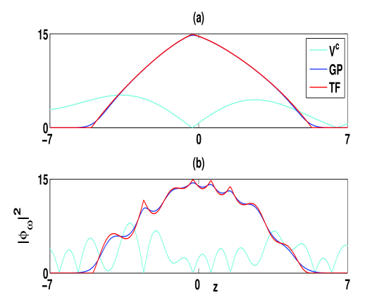
Figure 1: (a) Behavior of the condensate density $|\phi_{\omega}|^{2}$ obtained from the Thomas-Fermi approximation and from the Gross-Pitaevskii equation for a spatially slowly varying disordered potential characterized by $\lambda_{c}\approx 12\xi$. This corresponds to a weak disorder as compared to interactions. (b) Same plot but for a spatially rapidly varying disorder such that $\lambda_{c}\approx 2\xi$. The average disorder is kept much below the chemical potential ($\mu=30$) in both cases, so that $\langle s\rangle\ll 1$. We have taken $\alpha_{1d}=1$ and a number $N$ of bosons equal to $80$.

Generalizing the Thomas-Fermi approximation (7) so as to include the disorder $V^{c}$, we obtain for the corresponding density the expression,

$$\rho_{TF}(z) = \frac{\mu-z^{2}-V^{c}}{2\alpha_{1d}},~{}~{}\mu\geq z^{2}+V^{c}$$ (26)

$$= 0,~{}~{}\mu<z^{2}+V^{c}\,.$$

It is thus expected that this density presents local maxima and minima that follow the corresponding ones of the disordered potential. This trend is indeed very apparent in Fig.1. In Fig.1.(a), we consider a very smooth disorder such that $\lambda_{c}$ is much larger than the coherence length $\xi$ and we observe that apart from little deviations, the densities obtained from the Gross-Pitaevskii equation and from the Thomas-Fermi approximation match almost exactly as expected. Such a smooth disorder corresponds to the typical situations encountered in the experiments performed at Orsaydisorder3 , at LENSdisorder1a and Hannover sch05 . In Fig.1.(b), the disorder is stronger i.e. that it fluctuates on a smaller length scale $\lambda_{c}$ comparable to $\xi$, thus leading to more local minima and maxima of the disordered potential within the size of the cloud. The Gross-Pitaevskii density, obtained by solving (16), deviates from the Thomas-Fermi density at these extremal points. Moreover, we observe that the magnitude of those deviations gets larger when $\lambda_{c}$ gets smaller, i.e., for larger spatial variations of disorder. This behavior can be understood by considering the following expression for the density $\rho_{\omega}$

$$\rho_{\omega} = \frac{(\mu-z^{2}-V^{c}(z))}{2\alpha_{1d}}+\xi^{2}\left(\frac{\partial_{z}^{2}\phi}{\phi}\right)$$ (27)

$$= \rho_{TF}+\xi^{2}\left(\frac{\partial_{z}^{2}\phi}{\phi}\right)$$

which follows straightforwardly from Eq.(16). In this expression, the second term in the r.h.s., also known as quantum pressure term, is a correction to the Thomas-Fermi density whose origin is the zero point motion of the bosons in the condensate. This correction is proportional to the ratio $(\xi/\lambda_{c})^{2}$. It becomes larger for a decreasing $\lambda_{c}$, namely for a relatively larger effect of interactions driven by $\xi$. Thus a stronger disorder introduces more appreciable zero point motion of the bosons so as to reduce the interaction energy cost. In other words, the behavior of the static Thomas-Fermi condensate in a random potential is such that the disorder potential gets screened by the repulsive interaction sch05 ; SR94 .

Another feature of disorder is the spatial extension of the cloud defined, for a given disorder configuration, by

$$L_{\omega}=\sqrt{\overline{z^{2}}-\overline{z}^{2}}$$ (28)

where we have characterized the spatial distribution of the cloud by its moments,

$$\overline{z^{n}}=\frac{\int dzz^{n}\rho_{\omega}(z)}{\int dz\rho_{\omega}(z)}\,\ .$$ (29)

In Fig.2, we have plotted the configuration average $\langle L_{\omega}\rangle$ of the spatial extension as a function of the average strength $\mu\langle s\rangle$ (see Eq.17). The average spatial extension of the cloud, in the Thomas-Fermi limit is a decreasing function of the ratio $\lambda_{c}/\xi$, i.e., it decreases when interactions are getting larger than the spatial variation of disorder. We shall see that this behavior holds true even beyond the Thomas-Fermi approximation.

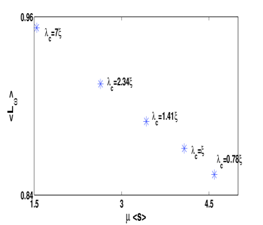
Figure 2: Plot of the width $\langle L_{\omega}\rangle$ averaged over disorder, as a function of the average strength $\mu\langle s\rangle$. $\langle L_{\omega}\rangle$ is expressed in units of the corresponding extension in the absence of disorder. For a given value of $\lambda_{c}$, we average over $200$ realizations of the disordered potential. Such calculations have been done for five different values of $\lambda_{c}$, the last one being less than the coherence length $\xi$ for which the validity of the mean-field theory is questionable. We have taken $\mu=30$ and $\alpha_{1d}=1$

IV.2 Time evolution

We study now the time evolution of the previous stationary solutions while switching off the trapping potential, but keeping the disordered potential. We then compare them with recent experiments and numerical calculations disorder1 ; disorder1a ; disorder3 ; modugno . In the experiments disorder2 ; sch05 , the BEC was prepared within the trapping and random potentials, but its expansion has been studied while switching off these potentials. This led to the observation of sharp fringes in the resulting density due to interference between different parts of the condensate. These conditions therefore differ from the case we consider.

We recall that our disorder is characterized by its strength $s$ in units of the chemical potential $\mu$ and by the length scale $\lambda_{c}$ of its spatial variations. The latter quantity is analogous to the correlation length of disorder defined in disorder3 . It is important to stress that in the Thomas-Fermi regime, the time evolution is very sensitive to the existence of potential barriers of height larger than the chemical potential $\mu$. If such a barrier exists, say at a point $z_{0}$, then we observe that the density $\rho_{\omega}(z)$ vanishes for $z\geq z_{0}$ at any subsequent times so that the cloud becomes spatially localized. Then, the average parameter $\langle s\rangle$ is not anymore relevant since it may be smaller than unity although some barriers may be larger than $\mu$. We thus need to characterize the disorder by means of higher moments. For a smooth enough probability distribution of the random variable $V_{m}\omega^{c}$, which is the case we consider, it is enough to consider the variance $\delta\omega^{c}$ defined by $\delta\omega^{c}=\left(\langle\left(\omega^{c}\right)^{2}\rangle-\langle\omega^{c}\rangle^{2}\right)^{1/2}$ and the parameter

$$\delta s={V_{m}\over\mu}\delta\omega^{c}$$ (30)

which sets the width of the distribution of potential barriers. In some of the cases we consider, the peak height of the disordered potential is twice as high as $V_{m}\delta_{\omega_{c}}$. A specific feature of one-dimensional disorder is that it is always very strong in contrast to higher dimensional systems for which the cloud may always find a way to avoid large potential barriers thus making effects of disorder comparatively weaker.

In Fig.3 we have plotted the density profile $\rho_{\omega}(T)$ after a time $T$ for different spatial variations of disorder. For instance, Figs.3(a) and (b) compare cases with different values of $\lambda_{c}$ but keeping the disorder strength $\delta s\ll 1$, almost unchanged. In contrast, Fig.3(a) and (c) display time evolutions for two disorder potentials having the same value of $\lambda_{c}$, but different strengths $\delta s$. In Fig.3(c), one of the potential well has a height almost equal to $\mu$. A first general observation is that for smaller values of $\lambda_{c}$, namely for stronger spatial fluctuations, the spatial expansion of the cloud is more inhibited, so that the main part of the cloud remains localized in finite regions that depend on the local landscape of the disordered potential. This trend is clearly apparent in Fig.3. On the other hand, for small values of $\delta s$, small amplitude density fluctuations extend far apart from the initial point whereas for large values of $\delta s$, density fluctuations do not extend beyond the closest barrier of height larger than $\mu$.

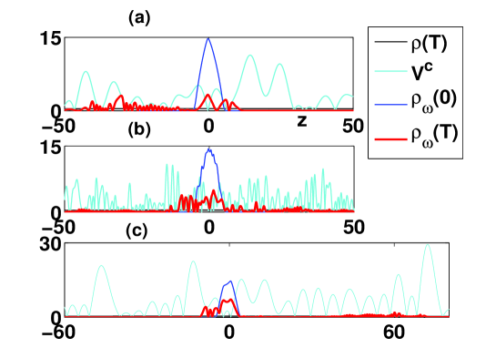
Figure 3: (a) Plot of the density profile $\rho_{\omega}=|\phi_{\omega}(z)|^{2}$ for two different times, $T=0$ and $T=25/\omega_{z}$ and for a slowly varying disorder such that $\lambda_{c}\approx 12\xi$. Both the average strength of the potential $\langle s\rangle=0.104$, and $\delta s=0.078$ are kept much below unity and $\mu=30$.The variables plotted in the vertical axis are indicated on the right hand side of the upper figure. The density profile in the absence of disorder at $T=25/\omega_{z}$ is shown in all three figures. The cloud extends almost uniformly. The horizontal axis label is indicated in the first figure only. (b) Time evolution of the density for a stronger spatial variation of disorder such that $\lambda_{c}\approx 2\xi$. $\langle s\rangle=0.095$ and $\delta s=0.076$ are kept well below unity ($\mu=30$). (c)Time evolution of the density for a stronger disorder characterized by $\langle s\rangle=0.23$, $\delta s=0.185$ and $\lambda_{c}=12\xi$. $\alpha_{1d}=1$ for all three plots

It has been pointed out in disorder3 that, during the time evolution of the Thomas-Fermi cloud, its center and its edge behave in a different way. After the trap potential is released, the density peak at the center, that corresponds to the highest value of the stationary density, gets lowered at an initial stage of the expansion. The interaction energy being larger than the kinetic energy, the density profile near the center still closely follows a Thomas-Fermi shape, but with a reduced chemical potential. The spatial variation of density fluctuations corresponds approximately to that of the disordered potential (that is of the order of $\lambda_{c}$). At the edges of the cloud, the density is lower so that the kinetic energy term takes over the interaction term and it is almost equal to the chemical potential $\mu$ of the condensate at $t=0$. Thus, the characteristic scale of spatial variations of density fluctuations at the edges of the cloud is the coherence length $\xi$ which is smaller than $\lambda_{c}$. This is displayed in Fig.4 which depicts the time evolution at the center ((a) and (b)) and at the edge ((c) and (d)). In Fig.4 (a), the center of the time evolved cloud follows the potential landscape and varies on a much larger length scale than the edge of the cloud. The other limit shown in Fig.4 ((b) and (d)), displays relatively less difference between spatial variations of density fluctuations at the center and at the edges of the cloud, since $\lambda_{c}\simeq\xi$.

In addition, Figs.4 describe how the matter wave behaves close to a single potential barrier, at the center and at the edge of the cloud. The shape of a typical potential is controlled by changing $\lambda_{c}$. In Figs.4 (a) and (b), it is shown how the central cloud becomes localized due to the presence of a potential barrier. The density modulation is driven by the the local potential landscape, rather than any interference effect. It has been pointed out in disorder1a ; modugno that the height of a single defect should vary like the energy $E$ of the incoming wavepacket over a distance short compared to its de Broglie wavelength in order to allow for quantum effects to dominate and eventually lead to Anderson localization. The potential used in our computation, generally does not satisfy this criterion. To satisfy it, one needs a disorder with higher $\delta s$ and lower $\lambda_{c}$. However under such conditions, the mean-field Gross-Pitaevskii approximation is questionable and the use of a discrete non-linear Schrödinger equation will be more appropriate.

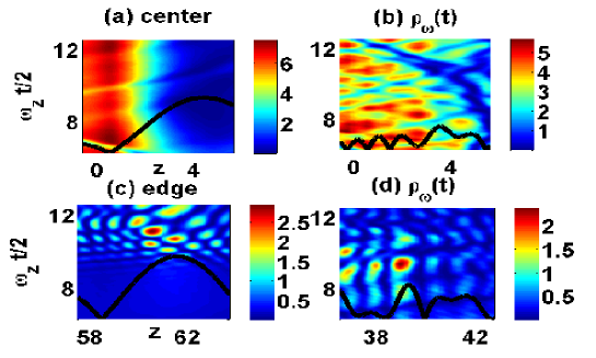
Figure 4: (a) and (c) Time evolution of the density at the center and at the edge for a strong disorder ( $\langle s\rangle=0.23$, $\delta s=0.185$ and $\lambda_{c}=12\xi$) identical to the one used in Fig.3(c). (b) and (d): Time evolution of the density at the center and at the edge for a disorder characterized by $\langle s\rangle=0.095$, $\delta s=0.076$ and $\lambda_{c}=2\xi$, identical to the one used in Fig.3(b). $\mu=30$ and $\alpha_{1d}=1$ for all figures. The horizontal, vertical and color-axis are the same for all three plots and are shown in alternative pair of figures. The black line in each figure shows the corresponding disordered potential. The potential is rescaled and its origin is shifted by the same amount in all figures to fit it in the size.

We have studied in Fig.5 the time evolution of the cloud density in momentum space and compare it to the cases without disorder and in the presence of an optical lattice. To make the comparison easier, we have used the amplitude of the optical lattice potential corresponding to that, $<s>+\delta s$, considered in Fig.5 (a). Fig.5 (a) shows a strong localization in $k$-space for high $\delta s$. This may be compared to the situation of Fig.5(d) (optical lattice). This strong localization occurs around the $k=0$ state. On the other hand when disorder fluctuates on a shorter scale $\lambda_{c}$ (with a smaller $\delta s$), a significant fraction of the density still occupies higher momentum states and the corresponding localization in momentum space is less pronounced. Thus, an experimental measurement of the momentum spectrum aspect2 of a quasi one-dimensional BEC in a disordered waveguide can shed light on the nature of localization of the cloud.

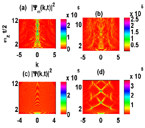
Figure 5: Density evolution in the $k-space$. Horizontal and vertical axis labels are identical for all the plots and are shown in (a). The color-axis label is indicated in (a) and (c). The four cases correspond to (a) Strong disorder as defined in Fig.3(c). (b) Weaker disorder fluctuating on a smaller length scale as defined in Fig.3 (b). (c) No disorder (d) Optical lattice: $(\langle s\rangle+\delta s)\sin\frac{2\pi z}{\lambda_{c}}$. The values of $\langle s\rangle$, $\delta s$ and $\lambda_{c}$ are those used in Fig.3(c).

After studying the time evolution of the density, we now discuss the time evolution of other properties of the cloud that characterize the suppression of its expansion. In Fig.6(a), the spatial extension $L_{\omega}$ for a given configuration, is plotted as a function of the dimensionless time $\omega_{z}t$. We observe that $L_{\omega}(t)$ saturates with time to a value which depends on the average strength $\langle s\rangle$ of the disorder.

In order to characterize this saturation, we define the ratio, denoted by $\cal R$, between the average kinetic and interaction energies of the cloud, defined by

$${\cal R}=2\xi^{2}{\int dz\left({\partial\phi_{\omega}\over\partial z}\right)^{2}\over\int dz|\phi_{\omega}|^{4}}\,\ .$$ (31)

In the stationary Thomas-Fermi approximation, the kinetic energy is almost negligible as compared to the interaction term, i.e., ${\cal R}\approx 0$. As the cloud expands, the interaction energy gets gradually converted into kinetic energy and this ratio increases. Finally, it saturates when almost all the interaction energy is converted into kinetic energy. This shows up in Fig.6(b). For a larger disorder, this increase of the ratio saturates more rapidly and the slope of $\cal R$, which indicates how fast the interaction energy is converted into kinetic energy, decreases. Particularly the lowest plot corresponding to a large disorder, shows a rapid saturation of $\cal{R}$ due to strong localization in momentum space. Since the edge of the cloud involves mostly kinetic energy, the behavior of $\cal R$ is dominated by the expansion of the central region. When the expansion is stopped by a potential barrier, the corresponding loss in kinetic energy is proportional to the height of the potential barrier. This explains the oscillations of $\cal R$ that appear in the presence of disorder.

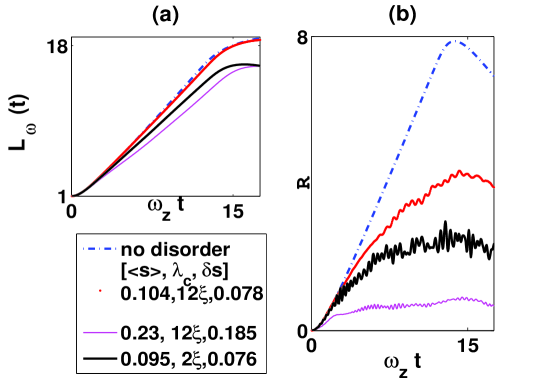
Figure 6: (a) Time evolution of the spatial extension $L_{\omega}(t)$ of the cloud as defined in (28) for a given configuration of the disordered potential but for different strengths $V_{m}$ and length scales $\lambda_{c}$. $\langle s\rangle$, $\lambda_{c}$ and $\delta s$ are indicated against each plot. $L_{\omega}(t)$ is expressed in units of its value at $t=0$. (b) Corresponding time evolution of the ratio $\cal R$ defined in (31).

V Gaussian limit

In this section we study effects of disorder on bosons that are condensed in the ground state of a harmonic oscillator potential. In that case, solutions of the Gross-Pitaevskii equation without disordered potential, are different from those observed in the Thomas-Fermi limit, and are given by Gaussian profiles centered at the origin. When the trap potential is released, corresponding time-dependent solutions remain Gaussian but with a larger width, a standard result from quantum mechanics (see Fig.7(a)).

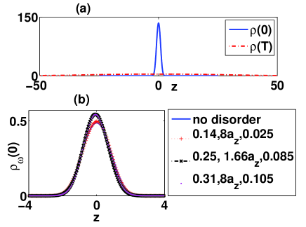
Figure 7: (a) Time evolution of the condensate density in the absence of disorder. $\rho(0)$ is the stationary density and $\rho(T)$ is the density after a time $T=\frac{25}{\omega_{z}}$. We have taken $\mu=2$ and $2\alpha_{1d}=0.01$ (b) Stationary profile of the condensate density in the presence of disorder. The corresponding values of the average disorder strength $\langle s\rangle$ , $\lambda_{c}$ and $\delta s$ are given in the inset.

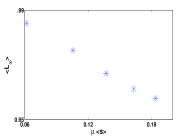
Figure 8: Plot of the disorder averaged width $\langle L_{\omega}\rangle$ of the stationary density profile in the Gaussian limit as a function of the average disorder strength $\mu\langle s\rangle$. The width is normalized by its value in the absence of disorder. For a given value of $\lambda_{c}$, the width is averaged over $200$ realizations of the potential. The values of $\lambda_{c}$ are those used in Fig.2 and, in units of the harmonic oscillator length $a_{z}$, they range between $0.55a_{z}$ (lowest point) and $5a_{z}$ (highest point). We have used $\mu=2$ and $2\alpha_{1d}=0.01$.

V.1 Stationary solutions

Like for the Thomas-Fermi regime, stationary solutions of the Gross-Pitaevski equation (16) in the presence of both trapping and disorder are characterized by the average strength $\langle s\rangle$ and the length $\lambda_{c}$. By changing the disorder strength we obtain behaviors such as those displayed in Fig. 7(b).

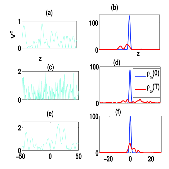
Figure 9: Left:(a,c,e) Plot of the disordered potential. The potentials in (a,e) vary on the same scale, whereas the potential in (c) varies on a smaller scale. The corresponding values of $\langle s\rangle$, $\lambda_{c}$ and $\delta s$ are respectively $(0.14,8a_{z},0.025)$, $(0.25,1.66a_{z},0.0846)$ and $(0.31,8a_{z},0.105)$. Right:(b,d,f) Time evolution of the density corresponding to the potentials plotted on the left. The initial stationary value of the density is denoted by $\rho_{\omega}(0)$ and $\rho_{\omega}(T)$ is computed at the time $T=25/\omega_{z}$. We have used $\mu=2$ and $2\alpha_{1d}=0.01$.

Since interaction effects are negligible in the Gaussian limit, the characteristic length of density variations is set by the harmonic oscillator length $a_{z}$, and not by the coherence length $\xi$ as before, the latter being very large in that case. In this regime dominated by confinement, we observe that the shape of the density profile depends weakly on disorder in contrast to the Thomas-Fermi limit, for which this profile follows the variations of the disorder. This is particularly apparent in Figures 9(c,d), where disorder varies over a length scale smaller than the width of the density profile without leading to fluctuations of this profile.

The density profile is well approximated by a off-centered Gaussian shape,

$$\rho_{\omega}(z)=A\exp\left(-\frac{(z-z_{0})^{2}}{L_{\omega}^{2}}\right)\,,$$ (32)

for a large range of disordered potentials (see Figure 7(b)). The amplitude $A$ and the width $L_{\omega}$ are related to each other through the normalization. The average width $\langle L_{\omega}\rangle$ is a decreasing function of the disorder strength $\mu\langle s\rangle$ defined by (17) as represented in Fig.8. Thus, the net effect of disorder is to spatially localize the bosons inside a narrower Gaussian.

V.2 Time dependent solutions

The behavior of the stationary condensate density profile in the presence of disorder in the Gaussian limit differs from the one obtained in the Thomas-Fermi limit. This difference shows up also in the time evolution of the density of the cloud after switching off the trapping potential. The short time expansion of the Thomas-Fermi cloud strongly depends on disorder, whereas in the Gaussian case, it does not. Moreover, in contrast to the Thomas-Fermi case, the zero point motion of the bosons is appreciable. The time evolution of the condensate density after switching off the trap is presented in Fig. 9 for different strengths of disorder.

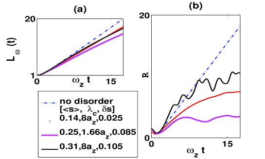
Figure 10: (a) Time evolution of the spatial extension $L_{\omega}(t)$ of the cloud for disorders of different strengths $V_{m}$ and length scales of variation $\lambda_{c}$. The disordered potentials are those used in Fig. 9 and the corresponding parameters are indicated ($\langle s\rangle$, $\lambda_{c}$, $\delta s$) in the inset. $L_{\omega}(t)$ is expressed in units of its value at $t=0$. (b) Corresponding time evolution of the ratio $\cal R$ defined in (31).

We first notice that on the same time scale, the density at the center of the cloud decreases more rapidly than for the Thomas-Fermi case (Figs.3 and 4). This results from the non negligible kinetic energy of a Gaussian cloud and the weaker interaction between bosons. Figure 10 displays the time evolution of the average spatial extension $\langle L_{\omega}\rangle$ of the cloud defined by (28) and the ratio of the average kinetic and interaction energies defined in (31). These two figures outline the difference between Thomas-Fermi and Gaussian time evolutions in the presence of disorder. The spatial extension in Fig.10(a) does not show any saturation over comparable time scales, though it grows at a lesser rate with increasing the strength of disorder. Correlatively, the ratio $\cal R$ in Figure 10(b) grows at a much faster rate and it takes a longer time to saturate. We can summarize these observations by saying that though the cloud expansion is indeed prevented by the disorder potential in the Gaussian regime, the suppression is weaker than in the Thomas-Fermi regime and it happens on longer time scales.

VI Soliton solutions for an attractive one-dimensional Bose-Einstein condensate

Having discussed the behavior of repulsive interacting bosons in the presence of disorder, we now turn to the case of an attractive solitonic condensate in similar situations. As we shall see, the change of the nature of the interaction modifies the behavior of the soliton solution with disorder as compared to the previous cases of Thomas-Fermi and Gaussian condensates. In contrast to Eq.(6) describing a repulsive interaction, Eq.(11) involves one free parameter only $(\alpha_{1d}=-1)$. As we have already mentioned, a change in $\alpha_{1d}$ only redefines the width of the soliton proportional to $1/\sqrt{\mu}$. In what follows, the width is always kept less than $\xi$.

VI.1 Stationary profiles

We start with the study of the stationary solutions of Eq.(11) with the addition of a random potential, namely,

$$-\mu\phi(z)+\partial_{z}^{2}\phi(z)+V_{d}\phi(z)+2|\phi|^{2}\phi=0\,\ .$$ (33)

It is important to notice that, in contrast with previous cases, there is no trapping potential, so that in the absence of disorder, the solution is invariant under translations. Numerically, we start with a randomly chosen initial guess which, once iterated, gives a solution located around the initial trial function. The overall shape of the stationary solution turns out to be independent of disorder, meaning that this shape can still be fitted with a function

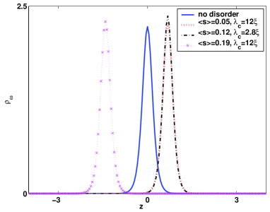
Figure 11: Stationary density profile of a bright soliton in the presence of disorder. The chemical potential is $\mu=-20$ and $\alpha_{1d}=-1$. The disordered potential is characterized by $|s|$ (since $\mu<0$) and $\lambda_{c}$. $<s>$ is the average of $|s|$.

of the type $A_{s}sech(B_{s}(z-z_{0}))$, where $A_{s}$ and $B_{s}=1/L_{\omega}$ are respectively the amplitude and the inverse width of the soliton. This feature appears clearly in Fig.(11) where the profile of the bright soliton has been plotted for several realizations of the potential. But, both the width and the amplitude depend on disorder as shown in Fig.(12) which displays the behavior of the width for an increasing strength of disorder. We have also checked the dependence upon length scales $\lambda_{c}$. Those features look similar to those obtained in the Gaussian limit. But they are essentially different. Whereas the soliton profile results from the comparison between kinetic and negative interaction energies, the Gaussian profile is obtained from the comparison between kinetic and confinement energies. This difference will manifest itself in the time evolution of the solitonic condensate.

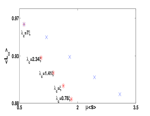
Figure 12: Disorder averaged width $\langle L_{\omega}\rangle$ of the stationary profile of a soliton as a function of the strength of disorder. For one set of points ($\times$), the strength $V_{m}$ of the disordered potential is increased keeping fixed the spatial scale of variation $\lambda_{c}$. For the other set of points ($*$), $\lambda_{c}$ is lowered which corresponds to stronger fluctuations of the disorder, while $V_{m}$ is kept fixed. $\langle L_{\omega}\rangle$ is expressed in units of its value in the absence of disorder and, for each case, it is averaged over $200$ realizations of the potential. The average potential is characterized by $|s|$ since $\mu<0$. The values of $\lambda_{c}$ are indicated in the figure. We have taken $\mu=-20$ and $2\alpha_{1d}=-1$.

VI.2 Time-dependent solutions

We now study the time evolution of the stationary solutions obtained previously, and not initial solutions given by (10) unlike the case considered in KIV90 . To this purpose, we first boost the soliton by giving it a finite (dimensionless) velocity $V_{s}=5$. In the absence of disorder, the soliton travels a distance $z=V_{s}T$ over a time $T$ without any change in its density profile. In the presence of a weak and smooth enough disorder, we observe that the soliton propagates retaining its initial ($t=0$) shape, over distances comparable to the non disordered case. A weak disorder potential has thus a negligible effect on the soliton motion. For a stronger disorder strength (i.e., for a smaller value of $\lambda_{c}$ and a larger value of $<s>$), the time behavior is displayed in Figures 13(a) and (b). In both cases, the soliton behaves classically and it becomes spatially localized, i.e. that it bounces back from high potential barriers typically higher than the kinetic energy. However, we do not observe a significant change in the shape of the soliton. Its width fluctuates as the soliton travels through the disordered potential and bounces back and forth. When the strength of disorder is higher, the soliton motion is clearly not linear (Figure 13(b)). This kind of motion can be qualitatively explained by considering the soliton as a massive classical particle of mass $mN$, where $m$ and $N$ are respectively the mass and the number of atoms in the condensate. Deviations from the linear motion result from the spatially varying force exerted on the soliton by the disorder potential. This kind of description is valid as long as the disorder potential remains smooth over the width of the soliton. Similar behaviors have been discussed in the context of soliton chaos in spatially periodic potentials martin , although the physical origin is different from the case discussed here. With the present stage of experiment soliton02 , such a behavior can be verified by studying the time evolution of a bright soliton in an optical speckle pattern.

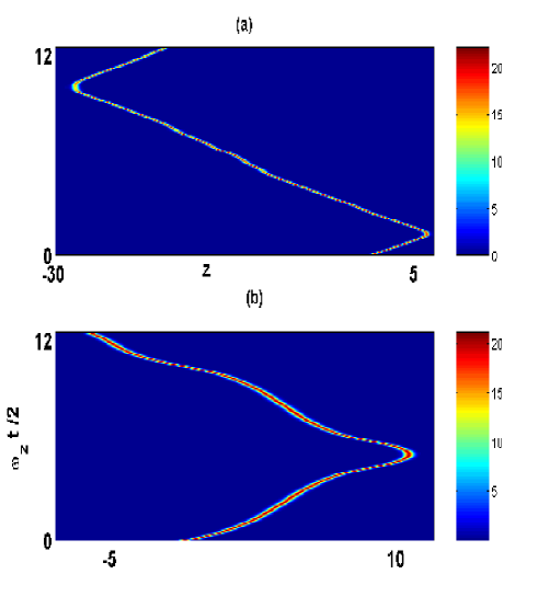
Figure 13: Time evolution of a boosted soliton in the presence of disorder. The chemical potential is $\mu=-20$, the dimensionless velocity at $t=0$ is $V_{s}=5$ and $\alpha_{1d}=-1$. The disorder potential is characterized by $|s|$ (since $\mu<0$) and $\lambda_{c}$. (a) Fastly varying disorder with $<s>=0.12$, $\delta s=0.162$ and $\lambda_{c}=2.8\xi$. (b) Stronger but slowly varying disorder with $<s>=0.19$, $\delta s=0.372$ and $\lambda_{c}=12\xi$.

VII Conclusion

We have performed a detailed numerical investigation of stationary solutions and time evolution of one dimensional Bose-Einstein condensates in the presence of a random potential. Stationary solutions which correspond either to the attractive interaction bright soliton or to repulsive interaction Gaussian matter waves with repulsive interactions in the regime where confinement dominates, behave in a qualitatively similar way. In contrast, the stationary solutions that correspond to a repulsive interacting Thomas-Fermi condensate, depend strongly on the strength of disorder and on its spatial scale of variations.

The time evolution of stationary solutions depends also significantly on the regime we consider. Although transport gets inhibited both for the attractive and repulsive interaction, this occurs in a very different way. For the repulsive case the center and the edge of the cloud behave differently and both are ultimately localized in a deep enough potential well. In the interaction dominated Thomas-Fermi regime, the main part of the cloud remains localized and edges that correspond to low densities and correlatively weaker interactions, propagate further away. A study of the corresponding momentum distribution of the cloud indicates a stronger localization of the matter wave in low momentum states for an increasing strength of the disorder potential. On the other hand, a moving bright soliton behaves very much like a single particle and it bounces back from a steep potential with its motion reversed. This behavior of a bright soliton may be contrasted against the behavior of a dark soliton in the presence of disorder which has been investigated recently NBNP05 .

For the values of the disorder strength and the non-linearity we have considered, we observe a behavior of solutions of the Gross-Pitaevskii equation that are mostly driven by the non-linearity, i.e., by interactions. Disorder plays mostly the role of a landscape within which a classical solution evolves in time. We did not observe, for the relatively large range of disorder and interaction parameters we have considered, a behavior close to Anderson localization, namely where spatially localized solutions result from interference effects. Since disorder is expected to be stronger in one-dimensional systems, we may conclude that, for the currently accessible experimental situations, Anderson localization effects will not be observable disorder1a ; sch05 ; SR94 due to the strength of the interaction term. Alternative setups are thus required in order to observe quantum localization of matter waves, having weak or zero interaction (e.g., by monitoring Feschbach resonances GC04 ).

The signature of Anderson localization in the nonlinear transport of a BEC in a wave-guide geometry has been studied in paul . There, the transmission coefficient has been shown to be exponentially decreasing with the system size below a critical interaction strength. But the different types of disorder and of the matter wave density at $t=0$, make a direct comparison with these results difficult.

VIII Acknowledgments

S. Ghosh thanks Hrvoje Buljan for his help in numerical computation. This research is supported in part by the Israel Academy of Sciences and by the Fund for Promotion of Research at the Technion.

References

- (1) P. W. Anderson, Phys. Rev. 109, 1492 (1958)
- (2) M. Belzons, E. Guazzelli and O. Parodi, J. of Fluid Mech. 186, 539 (1988); M. Belzons, P. Devillard, F. Dunlop, E. Guazzelli, O. Parodi and B. Souillard, Europhys. Lett. 4, 909 (1987)
- (3) C. Dépollier, J. Kergomard and F. Laloë, Ann. Phys. (France) 11, 457 (1986)
- (4) E. Akkermans and R. Maynard, J. Physique (France) , 1549 (1984)
- (5) E. Abrahams, P.W. Anderson, D. C. Licciardello, and T. V. Ramakrishnan, Phys. Rev. Lett. 42, 673 (1979).
- (6) A.A. Chabanov, M. Stoytchev and A.Z. Genack, Nature, 404, 850 (2000)
- (7) D.S. Wiersma, P. Bartolini, A. Lagendijk and R. Righini, Nature, 390, 671 (1997)
- (8) F. Scheffold, R. Lenke, R. Tweer and G. Maret, Nature 398, 207 (1999)
- (9) B. Kramer and A. MacKinnon, Rep. Prog. Phys. 56, 1469 (1993).
- (10) P.A. Lee and T.V. Ramakrishnan, Rev. Mod. Phys. 57, 287 (1985)
- (11) E. Akkermans and G. Montambaux, Physique mésoscopique des électrons et des photons, (Paris, EDP Sciences 2004). English translation (Cambridge University Press)
- (12) E. Akkermans and G. Montambaux, J. Opt. Soc. Am. B 21, 101 (2004)
- (13) P. Devillard and B. Souillard, J. of Stat. Phys. 43, 423 (1986).
- (14) B. Doucot and R. Rammal, Eur. Phys. Lett. 3, 969 (1987); ibid J. Phys. (Paris), 48, 527 (1987)
- (15) Y.S. Kivshar, S.A. Gredeskul, A. Sanchez and L. Vazquez, Phys. Rev. Lett. 64, 1693 (1990).
- (16) J.E. Lye, L. Fallani, M. Modugno, D. Wiersma, C. Fort and M. Inguscio, Phys. Rev. Lett. 95, 070401 (2005).
- (17) C. Fort, L. Fallani, V. Guarrera, J. Lye, M. Modugno, D. S. Wiersma and M. Inguscio, Phys. Rev. Lett. 95, 170410 (2005).
- (18) P. Kruger, L.M. Andersson, S. Wildermuth, S. Hofferberth, E. Haller, S. Aigner, S. Groth, I. Bar-Joseph, J. Schmiedmayer, arXiv:cond-mat/0504686.
- (19) D. Clément, A. F. Varón , M. Hugbart, J. Retter, P. Bouyer, L. Sanchez-Palencia, D.M. Gangardt, G. V. Shlyapnikov, A. Aspect, Phys. Rev. Lett. 95, 170409, (2005).
- (20) T. Schulte, S. Drenkelforth, J. Kruse, W. Ertmer, J. Arlt, K. Sacha, J. Zakrzewski., and M. Lewenstein, Phys. Rev. Lett. 95, 170411 (2005).
- (21) B. Damski, J. Zakrzewski, L. Santos, P. Zoller, and M. Lewenstein Phys. Rev. Lett. 91, 080403 (2003) and R. Pugatch, N. Bar-Gil, N. Katz, E Rowen and N. Davidson, arXiv:cond-mat/0603571.
- (22) A. Sanpera et al., Phys. Rev. Lett. 93, 040401 (2004).
- (23) D.W. Wang, M.D. Lukin, and E. Demler, Phys. Rev. Lett. 92, 076802 (2004).
- (24) U. Gavish and Y. Castin, Phys. Rev. Lett. 95, 020401 (2005).
- (25) B. Paredes, F. Verstraete and J.I. Cirac, Phys. Rev. Lett. 95, 140501 (2005).
- (26) N. Bilas and N. Pavloff, Phys. Rev. Lett. 95, 130403 (2005).
- (27) L. Fallani, J. Lye, V. Guarrera, C. Fort and M. Inguscio, arXiv:cond-mat/0603655.
- (28) M. Modugno, Phys. Rev. A 73, 013606 (2006).
- (29) T.Paul, P. Leboeuf, N. Pavloff, K. Richter and P. Schdagheck, Phys. Rev. A 72, 063621 (2005).
- (30) H. Gimperlein, S. Wessel, J. Schmiedmayer, and L. Santos, Phys. Rev. Lett. 95, 170401 (2005).
- (31) K. G. Singh and D. S. Rokshar, Phys. Rev. B 49, 9013 (1994).
- (32) M. Olshanii, Phys. Rev. Lett. 81, 938 (1998).
- (33) L. Pitaevskii and S. Stringari, Bose-Einstein condensation, Oxford (2003)
- (34) D.S. Petrov, G.V. Shlyapnikov and J.T.M. Walraven, Phys.Rev. Lett. 85, 3745 (2000) and D.M. Petrov, D.M. Gangardt and G.V. Shlyapnikov, J. Phys. IV France 1 (2004).
- (35) L. Tonks, Phys. Rev. 50, 955 (1967); M. D. Girardeau, J. Math. Phys. 1, 516 (1960); C. N. Yang and C. P. Yang, J. Math. Phys. 10, 1115 (1969).
- (36) L. Khaykovich et al., Science 296, 1290 (2002); K. E. Strecker et al., Nature 417, 150 (2002) and B. Eiermann et al. Phys. Rev. Lett. 92, 230401 (2004).
- (37) L.D. Carr and Y. Castin, Phys. Rev. A 66 063602 (2002).
- (38) C. Sulem and P. L. Sulem, The Nonlinear Schrödinger Equation Self-Focusing and Wave Collapse, Springer, New-York (1999).
- (39) V.I.Petviashvili, Sov. Plasma Phys. 2, 257 (1976).
- (40) M.J. Ablowitz and Z. H. Musslimani, Physica D, 184 276 (2003).
- (41) Z.H. Musslimani and J. Yang, J. Opt. Soc. Am. B 21, 973, (2004).
- (42) M.J. Ablowitz and Z. M. Musslimani Opt. Lett. 30, 2140 (2005).
- (43) W. Bao, D. Jaksch and P.A. Markowich, J. Comput. Phys. 187, 318 (2003)
- (44) S. Richard et al., Phys. Rev. Lett. 91, 010405 (2003).
- (45) R. Scharf and A.R. Bishop, Phys. Rev. A 46, R2973 (1992) and A.D. Martin, C.S. Adams and S.A. Gardinar, arXiv:cond-mat/0604086.