Doping-dependent evolution of low-energy excitations and quantum phase transitions within effective model for High-$T_{c}$ copper oxides

Abstract

In this paper a mean-field theory for the spin-liquid paramagnetic non-superconducting phase of the p- and n-type High-$T_{c}$ cuprates is developed. This theory applied to the effective $t-t^{\prime}-t^{\prime\prime}-J^{*}$ model with the ab initio calculated parameters and with the three-site correlated hoppings. The static spin-spin and kinematic correlation functions beyond Hubbard-I approximation are calculated self-consistently. The evolution of the Fermi surface and band dispersion is obtained for the wide range of doping concentrations $x$. For p-type systems the three different types of behavior are found and the transitions between these types are accompanied by the changes in the Fermi surface topology. Thus a quantum phase transitions take place at $x=0.15$ and at $x=0.23$. Due to the different Fermi surface topology we found for n-type cuprates only one quantum critical concentration, $x=0.2$. The calculated doping dependence of the nodal Fermi velocity and the effective mass are in good agreement with the experimental data.

I Introduction

Discovered almost 20 years ago, High-$T_{c}$ copper oxides still remain a challenge of the modern condensed matter physics. It is not only due to unconventional superconducting state with a highest superconducting transition temperature $T_{c}$ ever observed. Also they reveal evolution from an undoped antiferromagnetic (AFM) insulator to an almost conventional, though highly correlated nakamae2005 , Fermi liquid system at the overdoped side of the phase diagram. Between these two regimes the system exhibits strongly correlated, or so-called “pseudogap” metallic behavior up to an optimal doping concentration $x_{opt}\approx 0.16$.

Recent significant improvements of experimental techniques, especially of the Angle-Resolved Photoemission Spectroscopy (ARPES) and the Scanning Tunneling Microscopy (STM), revealed many exciting features of this doping dependent evolution. First of all, the Fermi surface (FS) at low doping concentrations $x$ has been measured shen2005 . Together with the previous measurements on optimally and overdoped samples (see e.g. review damascelli2003 and references therein), these observations provide a unified picture of the doping dependent FS, which changes from the “Fermi arcs” yoshida2003 in the underdoped compounds to the “large” Fermi surface in the overdoped systems. Though this change is smooth, it occurs around the optimal doping concentration. Also, the observed evolution is consistent with the Hall coefficient $R_{H}$ measurements ando2004RH .

The pseudogap behavior observed in ARPES is also tracked in the transport measurements. In particular, the resistivity curvature mapping over $T-x$ phase diagram clearly demonstrates crossover between underdoped and overdoped regimes ando2004 . And the in-plane resistivity $\rho_{ab}$ shows $T$-linear dependence only around $x_{opt}$.

The drastic change of the quasiparticle dynamics around the optimal doping was found by the time-resolved measurements of the photoinduced change in reflectivity for Bi₂Sr₂Ca_1-yDy_yCu₂O_8+δ (BSCCO) gedik2005 . Namely, the spectral weight shifts expected for a BCS superconductor can account for the photoinduced response in overdoped, but not underdoped BSCCO. This agrees with the observed difference of the low-frequency spectral weight transfer in normal and superconducting states on under- and over-doped samples bontemps2004 ; carbone2006 .

Meanwhile, the integral characteristics of the system demonstrate more smooth behavior upon increase of the doping $x$. The dependence of the chemical potential shift $\Delta\mu$ on $x$ shows pinning at $x<x_{opt}$, and evolves smoothly at higher doping concentrations harima2001 . The measured nodal Fermi velocity $v_{F}$ is almost doping-independent within experimental error of 20% zhou2003 ; kordyuk2005 . The experiments involving combination of dc transport and infrared spectroscopy revealed an almost constant effective electron mass $m^{*}/m=3.8\pm 2$ in the underdoped and slightly overdoped La_2-xSr_xCuO₄ (LSCO) and YBa₂Cu₆O_y (YBCO) padilla2005 . Low-$x$ effective mass dependence contradicts predictions of the Brinkman-Rice metal-insulator transition theory brinkman1970 , predicting divergence of the $m^{*}$ at the point of transition. One of the main drawbacks in this theory is that the magnetic correlations were neglected. Thus the discrepancy with the experiment emphasizes the importance of these correlations in High-$T_{c}$ copper oxides.

From the theoretical point of view, the description of the crossover between almost localized picture and the Fermi liquid regime is very difficult. Starting from the Fermi liquid approach one may discuss the overdoped and, partly, optimally doped region, while for underdoped and undoped samples this approach is not applicable. The strong-coupling Gutzwiller approximation gutzwiller1963 for the Hubbard model provides a good description for the correlated metallic system. This approximation is equivalent gebhard1990 ; gebhard1991 to the mean-field saddle-point solution within a slave-boson approach kotliar1986 . At the same time, as shown within $1/d$ expansion gebhard1990 , with $d$ being the dimensionality of the lattice, the Gutzwiller approximation is equivalent to the case of $d=\infty$. Obviously, for the quasi-two-dimensional systems such as High-$T_{c}$ copper oxides this is not a proper limit. The same applies to the Dynamical Mean-Field Theory (DMFT) metzner1989 ; georges1996 , which is exact only for $d=\infty$. In this limit the short-range magnetic fluctuations are excluded. It is not a good starting point for the system with long-range AFM order at low $x$ and short-range AFM correlations in the underdoped region.

To describe the doping dependent evolution of the low-energy excitations we develop a strong-coupling mean-field theory for the paramagnetic non-superconductive phase of High-$T_{c}$ copper oxides starting from the local limit. To go beyond the usual Hubbard-I approximation a self-consistently calculated static spin-spin and kinematic correlation functions are taken into account. Within this approximation in the framework of the effective $t-t^{\prime}-t^{\prime\prime}-J^{*}$ model with ab initio calculated parameters we obtain a doping-dependent evolution of the FS, effective mass and nodal Fermi velocity. The analysis of the low-energy excitations behavior for p-type cuprates yields two quantum phase transitions associated with the change of the FS topology. For n-type cuprates we observe only single quantum critical concentration. The key aspect in these findings is an adequate description of the electron scattering by the short range magnetic fluctuations accompanied by the three-site correlated hoppings.

The paper is organized as follows. In Section II the effective model and the approximations are described. The results of the calculations for p-type cuprates are presented in Section III. Also, the critical comparison of the $t-t^{\prime}-t^{\prime\prime}-J^{*}$ and $t-t^{\prime}-t^{\prime\prime}-J$ models is made, and the role of short range magnetic order is discussed. Section IV contains results for n-type cuprates. The last Section summarize this study, and the main points are discussed.

II Model and Approximations

High-$T_{c}$ cuprates belong to a class of strongly correlated systems where the standard local density approximation (LDA) schemes and the weak-coupling perturbation theories yield an inappropriate results. To overcome this difficulty recently we have developed an LDA+GTB method korshunov2005 . In this method the ab initio LDA calculation is used to construct the Wannier functions and to obtain the single electron and Coulomb parameters of the multiband Hubbard-type model. Within this model the electronic structure in the strong correlation regime is calculated by the Generalized Tight-Binding (GTB) method ovchinnikov1989 ; gavrichkov2000 . The latter combines the exact diagonalization of the model Hamiltonian for a small cluster (unit cell) with perturbative treatment of the intercluster hopping and interactions. For undoped and weakly doped LSCO and Nd_2-xCe_xCuO₄ (NCCO) this scheme results in a charge transfer insulator with a correct value of the gap and the dispersion of bands in agreement with the experimental ARPES data (see Ref. korshunov2005 for details).

Then this multiband Hubbard-type Hamiltonian was mapped onto an effective low-energy model korshunov2005 . Parameters of this effective model were obtained directly from the ab initio parameters of the multiband model. The low-energy model appears to be the $t-t^{\prime}-t^{\prime\prime}-J^{*}$ model ($t-t^{\prime}-t^{\prime\prime}-J$ model with the three-site correlated hoppings) for n-type cuprates and the singlet-triplet $t-t^{\prime}-t^{\prime\prime}-J^{*}$ model for p-type systems. However, for $x<0.7$ in a phase without a long-range magnetic order the role of the triplet state and the singlet-triplet hybridization is negligible korshunov2006 . Therefore, the triplet state could be omitted and in the present paper we will describe the low-energy excitations in the single-layer p- and n-type cuprates within the $t-t^{\prime}-t^{\prime\prime}-J^{*}$ model.

To write down the model Hamiltonian we use the Hubbard $X$-operators hubbard1964 : $X_{f}^{\alpha}\leftrightarrow X_{f}^{n,n^{\prime}}\equiv\left|n\right>\left<n^{\prime}\right|$. Here index $\alpha\leftrightarrow(n,n^{\prime})$ enumerates quasiparticle with energy $\omega_{\alpha}=\varepsilon_{n}(N+1)-\varepsilon_{n^{\prime}}(N)$, where $\varepsilon_{n}$ is the $n$-th energy level of the $N$-electron system. The commutation relations between X-operators are quite complicated, i.e. two operators commute on another operator, not a $c$-number. Nevertheless, depending on the difference of the number of fermions in states $n$ and $n^{\prime}$ it is possible to define quasi-Fermi and quasi-Bose type operators in terms of obeyed statistics. In this notations the Hamiltonian of the $t-t^{\prime}-t^{\prime\prime}-J^{*}$ model in the hole representation have the form:

$$H = \sum_{f,\sigma}\left(\varepsilon_{0}-\mu\right)X_{f}^{\sigma,\sigma}+\sum_{f\neq g,\sigma}t_{fg}X_{f}^{\sigma,0}X_{g}^{0,\sigma}$$ (1)

$$+ \sum_{f\neq g}J_{fg}\left(\vec{S}_{f}\vec{S}_{g}-\frac{1}{4}n_{f}n_{g}\right)+H_{3}.$$

Here $\mu$ is the chemical potential, $\vec{S}_{f}$ is the spin operator, $S_{f}^{+}=X_{f}^{\sigma,\bar{\sigma}}$, $S_{f}^{-}=X_{f}^{\bar{\sigma},\sigma}$, $S_{f}^{z}=\frac{1}{2}\left(X_{f}^{\sigma,\sigma}-X_{f}^{\bar{\sigma},\bar{\sigma}}\right)$, $n_{f}=\sum\limits_{\sigma}X_{f}^{\sigma,\sigma}$ is the number of particles operator, $J_{fg}=2\tilde{t}_{fg}^{2}/E_{ct}$ is the exchange parameter, $E_{ct}$ is the charge-transfer gap. In the notations of Ref. korshunov2005 the hopping matrix elements $t_{fg}$ corresponds to $t_{fg}^{SS}$ and $-t_{fg}^{00}$ for p- and n-type cuprates, respectively, and $\tilde{t}_{fg}=t_{fg}^{0S}$. Hamiltonian $H_{3}$ contains the three-site interaction terms:

$$H_{3}=\sum\limits_{f\neq g\neq m,\sigma}\frac{\tilde{t}_{fm}\tilde{t}_{mg}}{E_{ct}}\left(X_{f}^{\sigma 0}X_{m}^{\bar{\sigma}\sigma}X_{g}^{0\bar{\sigma}}-X_{f}^{\sigma 0}X_{m}^{\bar{\sigma}\bar{\sigma}}X_{g}^{0\sigma}\right).$$ (2)

There is a simple correspondence between $X$-operators and single-electron annihilation operators: $a_{f\lambda\sigma}=\sum\limits_{\alpha}\gamma_{\lambda\sigma}(\alpha)X_{f}^{\alpha}$, where the coefficients $\gamma_{\lambda\sigma}(\alpha)$ determines the partial weight of the quasiparticle $\alpha$ with spin $\sigma$ and orbital index $\lambda$. These coefficients are calculated straightforwardly within the GTB scheme. In the considered case there is only one quasi-Fermi-type quasiparticle, $\alpha=(0,\sigma)$, with $\gamma_{\lambda\sigma}(\alpha)=1$, and the Hamiltonian in the generalized form in momentum representation is given by:

$$H = \sum\limits_{\vec{k},\sigma}\left(\varepsilon_{0}-\mu\right)X^{\sigma,\sigma}_{\vec{k}}+\sum\limits_{\vec{k}}\sum\limits_{\alpha,\beta}t_{\vec{k}}^{\alpha\beta}{X_{\vec{k}}^{\alpha}}^{\dagger}X_{\vec{k}}^{\beta}$$ (3)

$$+ \sum\limits_{\vec{p},\vec{q}}\sum\limits_{\alpha,\beta,\sigma,\sigma^{\prime}}V_{\vec{p}\vec{q}}^{\alpha\beta,\sigma\sigma^{\prime}}{X_{\vec{p}}^{\alpha}}^{\dagger}X_{\vec{p}-\vec{q}}^{\sigma,\sigma^{\prime}}X_{\vec{q}}^{\beta}.$$

The Fourier transform of the two-time retarded Green function in the energy representation, $G_{\lambda}(\vec{k},E)=\left<\left<a_{\vec{k}\lambda\sigma}\left|a_{\vec{k}\lambda\sigma}^{\dagger}\right.\right>\right>_{E}$, can be rewritten in terms of the matrix Green function $\left[\hat{D}(\vec{k},E)\right]_{\alpha\beta}=\left<\left<X_{\vec{k}}^{\alpha}\left|{X_{\vec{k}}^{\beta}}^{\dagger}\right.\right>\right>_{E}$:

$$G_{\lambda}(\vec{k},E)=\sum\limits_{\alpha,\beta}\gamma_{\lambda\sigma}(\alpha)\gamma_{\lambda\sigma}^{*}(\beta)D^{\alpha\beta}({\vec{k}},E).$$ (4)

The diagram technique for Hubbard X-operators has been developed zaitsev1975 ; izumov1991 and the generalized Dyson equation ovchinnikov_book2004 in the paramagnetic phase ($\left<X_{0}^{\sigma,\sigma}\right>=\left<X_{0}^{\bar{\sigma},\bar{\sigma}}\right>$) reads:

$$\hat{D}(\vec{k},E) = \left[\hat{G}_{0}^{-1}(E)-\hat{P}(\vec{k},E)\hat{t}_{\vec{k}}-\hat{P}(\vec{k},E)\hat{V}_{\vec{k}\vec{k}}^{\sigma,\sigma}\left<X_{0}^{\sigma,\sigma}\right>\right.$$ (5)

$$+ \left.\hat{\Sigma}(\vec{k},E)\right]^{-1}\hat{P}(\vec{k},E).$$

Here, $\hat{G}_{0}^{-1}(E)$ is the exact local Green function, $G_{0}^{\alpha\beta}(E)=\delta_{\alpha\beta}/\left[{E-\left({\varepsilon_{n}-\varepsilon_{n^{\prime}}}\right)}\right]$, $\hat{\Sigma}(\vec{k},E)$ and $\hat{P}(\vec{k},E)$ are the self-energy and the strength operators, respectively. The presence of the strength operator is due to the redistribution of the spectral weight between the Hubbard subbands, that is an intrinsic feature of the strongly correlated electron systems. It also should be stressed that $\hat{\Sigma}(\vec{k},E)$ in Eq. (5) is the self-energy in $X$-operators representation and therefore it differs from the self-energy entering Dyson equation for the weak coupling perturbation theory for $G_{\lambda}(\vec{k},E)$.

Within Hubbard-I approximation hubbard1963 the self-energy $\hat{\Sigma}(\vec{k},E)$ is equal to zero and the strength operator $\hat{P}(\vec{k},E)$ is replaced by $P^{\alpha\beta}(\vec{k},E)\to P^{\alpha\beta}=\delta_{\alpha\beta}F_{\alpha}$, where $F_{\alpha(n,n^{\prime})}=\left<X_{f}^{n,n}\right>+\left<X_{f}^{n^{\prime},n^{\prime}}\right>$ is the occupation factor.

Taking into account that in the considered paramagnetic phase $\left<X_{f}^{\sigma,\sigma}\right>=\frac{1-x}{2}$, $\left<X_{f}^{0,0}\right>=x$, with $x$ being the doping concentration, after all substitutions and treating all $\vec{k}$-independent terms as the chemical potential renormalization, the generalized Dyson equation for the Hamiltonian (1) becomes:

$$D(\vec{k},E) = \left[E-(\varepsilon_{0}-\mu)-\frac{1+x}{2}t_{\vec{k}}\right.$$ (6)

$$- \left.\frac{1+x}{2}\frac{\tilde{t}_{\vec{k}}^{2}}{E_{ct}}\frac{1-x}{2}+\Sigma(\vec{k},E)\right]^{-1}\frac{1+x}{2}.$$

To go beyond the Hubbard-I approximation we have to calculate $\Sigma(\vec{k},E)$. For this purpose we use an equations of motion method for the $X$-operators plakida1989 . The exact equation of motion for $X_{k}^{\alpha}$ is:

$$i\dot{X}_{\vec{k}}^{\alpha} = \left[X_{\vec{k}}^{\alpha},H\right]=(\varepsilon_{0}-\mu)X_{\vec{k}}^{\alpha}+L_{\vec{k}}^{\alpha}$$ (7)

$$= (\varepsilon_{0}-\mu)X_{\vec{k}}^{\alpha}+{L_{\vec{k}}^{\alpha}}^{(0)}+(L_{\vec{k}}^{\alpha}-{L_{\vec{k}}^{\alpha}}^{(0)}).$$

Here ${L_{\vec{k}}^{\alpha}}^{(0)}$ is the linearized and decoupled in Hubbard-I approximation operator $L_{\vec{k}}^{\alpha}$,

$${L_{\vec{k}}^{\alpha}}^{(0)}=\frac{1+x}{2}t_{\vec{k}}+\frac{1+x}{2}\frac{\tilde{t}_{\vec{k}}^{2}}{E_{ct}}\frac{1-x}{2}.$$ (8)

Let us define $\tilde{L}_{\vec{k}}^{\alpha}=L_{\vec{k}}^{\alpha}-{L_{\vec{k}}^{\alpha}}^{(0)}$ and linearize it with respect to $X_{\vec{k}}^{\alpha}$:

$$\tilde{L}_{\vec{k}}^{\alpha}=\sum\limits_{\beta}T_{\vec{k}}^{\alpha\beta}X_{\vec{k}}^{\beta}+\tilde{L}_{\vec{k}}^{\alpha(irr)},$$ (9)

where $T_{\vec{k}}^{\alpha\beta}=\frac{\left<\left\{\tilde{L}_{\vec{k}}^{\alpha},{X_{\vec{k}}^{\beta}}^{\dagger}\right\}\right>}{\left<\left\{X_{\vec{k}}^{\beta},{X_{\vec{k}}^{\beta}}^{\dagger}\right\}\right>}$ are the coefficients of the linearization. All effects of the finite quasiparticle lifetime are contained in the irreducible part $\tilde{L}_{\vec{k}}^{\alpha(irr)}$. In this paper we neglect it, $\tilde{L}_{\vec{k}}^{\alpha(irr)}\to 0$.

Since the exact equation for the Green function is given by $E\left<\left<X_{\vec{k}}^{\alpha}\left|{X_{\vec{k}}^{\beta}}^{\dagger}\right.\right>\right>_{E}=\left<\left\{X_{\vec{k}}^{\alpha},{X_{\vec{k}}^{\beta}}^{\dagger}\right\}\right>+\left<\left<i\dot{X}_{\vec{k}}^{\alpha}\left|{X_{\vec{k}}^{\beta}}^{\dagger}\right.\right>\right>_{E}$, it is straightforward to find that in our approximation $T_{\vec{k}}^{\alpha\beta}$ corresponds to the self-energy:

$$\hat{\Sigma}(\vec{k},E)=-\hat{T}_{\vec{k}}.$$ (10)

Introducing notations for the static spin-spin correlation functions

$$C_{\vec{q}}=\sum\limits_{f,g}e^{-i(f-g)\vec{q}}\left<X_{f}^{\sigma\bar{\sigma}}X_{g}^{\bar{\sigma}\sigma}\right>=2\sum\limits_{\vec{r}}e^{-i\vec{r}\vec{q}}\left<S_{\vec{r}}^{z}S_{0}^{z}\right>,$$ (11)

and for the kinematic correlation functions

$$K_{\vec{q}}=\sum\limits_{f,g}e^{-i(f-g){\vec{q}}}\left<X_{f}^{\sigma 0}X_{g}^{0\sigma}\right>,$$ (12)

the expression for the quasiparticle self-energy becomes:

$$\Sigma(\vec{k},E) = \frac{2}{1+x}\frac{1}{N}\sum\limits_{\vec{q}}\left[t_{\vec{q}}-\frac{1-x}{2}J_{\vec{k}-\vec{q}}-x\frac{\tilde{t}_{\vec{q}}^{2}}{E_{ct}}-\frac{1+x}{2}\frac{2\tilde{t}_{\vec{k}}\tilde{t}_{\vec{q}}}{E_{ct}}\right]K_{\vec{q}}$$ (13)

$$- \frac{2}{1+x}\frac{1}{N}\sum\limits_{\vec{q}}\left[t_{\vec{k}-\vec{q}}-\frac{1-x}{2}\left(J_{\vec{q}}-\frac{\tilde{t}_{\vec{k}-\vec{q}}^{2}}{E_{ct}}\right)-\frac{1+x}{2}\frac{2\tilde{t}_{k}\tilde{t}_{\vec{k}-\vec{q}}}{E_{ct}}\right]\frac{3}{2}C_{\vec{q}}.$$

Here $N$ is the number of vectors in momentum space.

Until now we have made two major approximations. First, we neglected irreducible part of the self-energy, $\tilde{L}_{\vec{k}}^{\alpha(irr)}$, thus allowing quasiparticles to have infinite lifetime. Second, and this is not so obvious, in Eq. (6) for the strength operator $\hat{P}(\vec{k},E)$ we drop out corrections beyond Hubbard-I approximation. These dropped corrections also lead to the finite quasiparticle lifetime. The consequence of these approximations will be discussed later.

Kinematic correlation functions (12) are calculated straightforwardly with the help of Green function (6). The spin-spin correlation functions for the $t-J$ model with three-site correlated hoppings $H_{3}$ were calculated in Ref. valkov2005 . In this paper the equations of motion for the spin-spin Green function $\left<\left<X_{f}^{\sigma\bar{\sigma}}\left|X_{g}^{\bar{\sigma}\sigma}\right.\right>\right>_{\omega}$ were decoupled in the rotationally invariant quantum spin liquid phase, similar to Refs. shimahara1991 ; barabanov1992 . The results of this approach for a static magnetic susceptibility for the $t-J$ model are similar to those obtained by other methods sherman2002 ; vladimirov2005 . Higher-order correlation functions appearing due to the $H_{3}$ term are decoupled in the following way:

$$\left<\left<X_{m}^{\bar{\sigma}\bar{\sigma}}X_{n}^{\sigma 0}X_{l}^{0\bar{\sigma}}\left|\right.X_{j}^{\bar{\sigma}\sigma}\right>\right>_{\omega}\to\left<X_{m}^{\bar{\sigma}\bar{\sigma}}\right>\left<\left<X_{n}^{\sigma 0}X_{l}^{0\bar{\sigma}}\left|\right.X_{j}^{\bar{\sigma}\sigma}\right>\right>_{\omega}$$

$$\left<\left<X_{m}^{\sigma\bar{\sigma}}X_{l}^{\sigma 0}X_{n}^{0\sigma}\left|\right.X_{j}^{\bar{\sigma}\sigma}\right>\right>_{\omega}\to\left<X_{l}^{\sigma 0}X_{n}^{0\sigma}\right>\left<\left<X_{m}^{\sigma\bar{\sigma}}\left|\right.X_{j}^{\bar{\sigma}\sigma}\right>\right>_{\omega}$$

Thus, higher-order kinematic and spin-spin scattering channels are decoupled.

After the terms proportional to $x\left(2\tilde{t}_{01}/E_{ct}\right)^{2}$ being neglected, the expression for Fourier transform of the spin-spin Green function becomes:

$$\left<\left<X_{\vec{q}}^{\sigma\bar{\sigma}}\left|\right.X_{\vec{q}}^{\bar{\sigma}\sigma}\right>\right>_{\omega}=\frac{A_{\vec{q}}(\omega)}{\omega^{2}-\omega_{\vec{q}}^{2}},$$ (14)

where

$$A_{\vec{q}}(\omega) = \frac{1}{N}\sum\limits_{\vec{k}}\left[\left(-2t_{\vec{k}}+\frac{1-x}{2}\frac{\tilde{t}_{k}^{2}}{E_{ct}}\right)\left(K_{\vec{k}}-K_{\vec{q}-\vec{k}}\right)\right.$$ (15)

$$+ \left.4J_{\vec{k}}\left(C_{\vec{q}-\vec{k}}-C_{\vec{k}}\right)\right],$$

and magnetic excitations spectrum $\omega_{\vec{q}}$ represented by the Eq. (26) of paper valkov2005 .

The following results were obtained by self-consistent calculation of the chemical potential $\mu$, the spin-spin correlation functions (11) using Green function (14), and the kinematic correlation functions (12) using Green function (6) with the self-energy (13).

III Results for p-type cuprates

For LSCO the LDA+GTB calculated parameters are (in eV): $t=0.93,t^{\prime}=-0.12,t^{\prime\prime}=0.15,J=0.295,J^{\prime}=0.003,J^{\prime\prime}=0.007$. All figures below are in electron representation.

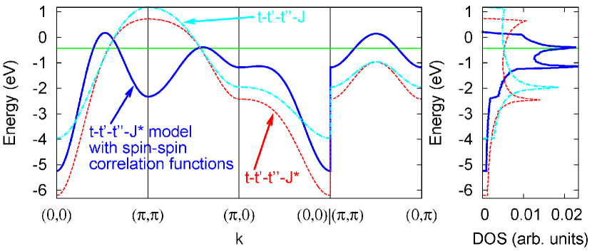
Figure 1: (color online) The quasiparticle dispersion (on the left) and the density of states (DOS, on the right) in the paramagnetic phase of p-type cuprate with $x=0.16$. The position of the chemical potential is denoted by the horizontal (green) line. Results within the Hubbard-I approximation are shown by dashed (red) and dash-dotted (cyan) curves for the model with ($t-t^{\prime}-t^{\prime\prime}-J^{*}$ model) and without ($t-t^{\prime}-t^{\prime\prime}-J$ model) three-site correlated hoppings, respectively. Bold solid (blue) curves represent the results for the $t-t^{\prime}-t^{\prime\prime}-J^{*}$ model with the short range magnetic order.

First of all we would like to stress the important effects caused by the three-site correlated hoppings $H_{3}$ and the renormalizations due to the short range magnetic order. Previously, the importance of the three-site correlated hoppings in the normal and superconducting phases has been demonstrated in Refs. valkov2005 ; valkov2002 ; korshunov2004 . In Fig. 1 we present our results for 16% hole doping within different approximations. Evidently, introduction of three-site interaction terms results in the change of the position of the top of the valence band. Therefore, this will become important at small $x$. In AFM phase of the $t-J$ model there is a symmetry around $(\pi/2,\pi/2)$ point. In the paramagnetic phase this symmetry is absent. Due to the scattering on the short range magnetic fluctuations with AFM wave vector $\vec{Q}=(\pi,\pi)$ the states near the $(\pi,\pi)$ point are pushed below the Fermi level (see Fig.1), thus totally changing the shape of the FS. In other words, the short range magnetic order “tries” to restore the symmetry around $(\pi/2,\pi/2)$ point. In our calculations the short range magnetic fluctuations are taken into account via the spin-spin correlation functions (11).

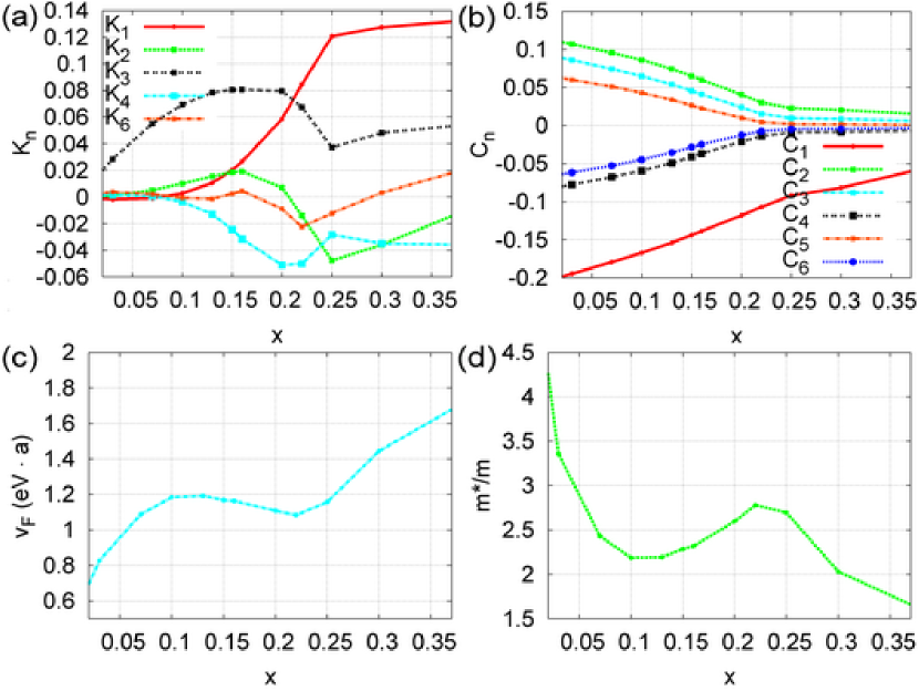
Figure 2: (color online) Doping dependent evolution of the kinematic (a) and spin-spin (b) correlation functions within the $t-t^{\prime}-t^{\prime\prime}-J^{*}$ model for p-type cuprates. Index $n$ enumerates real space vectors connecting neighboring sites: $n=1$ for nearest-neighbors, $n=2$ for the next nearest neighbors, and so on. In (c) and (d) the doping dependence of the nodal Fermi velocity (in units of eV$\cdot a$ with $a$ being a lattice constant) and the effective mass are shown.

Our results for the doping dependence of the kinematic and spin-spin correlation functions are shown in Fig. 2. Note, the kinematic correlation functions $K_{n}$ possess a very nontrivial doping dependence. For low concentrations, $x<0.15$, due to the strong magnetic correlations the hoppings to the nearest and to the next-nearest neighbors are suppressed leading to the small values of $K_{1}$ and $K_{2}$, while $K_{3}$ is not suppressed. Upon increase of the doping concentration above $x\approx 0.15$, magnetic correlations decrease considerably and nearest-neighbor kinematic correlation function $K_{1}$ increase. Next major change sets at $x\approx 0.23$ when the system possesses almost Fermi liquid behavior: $K_{1}$ becomes largest of all $K_{n}$’s, while the magnetic correlation functions $C_{n}$ and the kinematic correlation function $K_{3}$ are strongly suppressed.

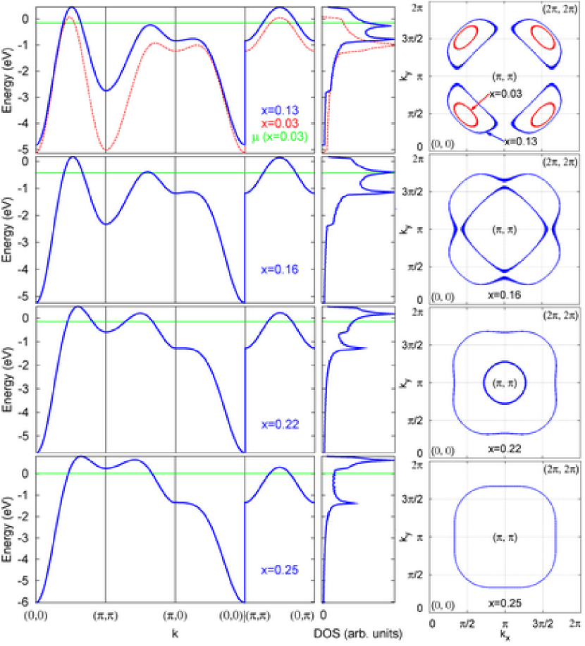
Figure 3: (color online) Band structure (on the left), density of states (in the middle), and Fermi surface (on the right) evolution with doping concentration $x$ within the $t-t^{\prime}-t^{\prime\prime}-J^{*}$ model for p-type cuprates.

So, we can clearly define two points of the crossover, namely $x\approx 0.15$ and $x\approx 0.23$. The system behavior is quite different on the different sides of these points, although there is no phase transition with symmetry breaking occurs. To understand the nature of these crossovers we consider the FS evolution with doping concentration, presented in Fig.3. At low $x$ the FS has the form of the hole pockets centered around $(\pm\pi/2,\pm\pi/2)$ point. Then these pockets enlarge and at $x=0.15$ all of them merge together, forming the two FS contours. Up to $x=0.23$ the FS topologically equivalent to the two concentric circles with the central one shrinking toward $(0,0)$ point. For $x=0.23$ the central FS contour shrinks to the single point and vanishes, leaving one large hole-type FS.

Apparently, the topology of the FS changes drastically upon doping. In particular, it happens at $x=0.15$ and at $x=0.23$. For the first time the “electronic transition” accompanying the change in the FS topology, or the so-called Lifshitz transition, was described in Ref. lifshitz1960 . Now such transitions referred as a quantum phase transitions with a co-dimension$=1$ (see e.g. paper volovik2006 ). Note, when the FS topology changes at quantum critical concentrations $x_{1}=0.15$ and at $x_{2}=0.23$ the density of states at the Fermi level also exhibit significant modifications. This results in the different behavior of the kinematic and magnetic correlation functions on the different sides of these crossover points. And the changes in the density of states at the Fermi level will also result in the significant changes of such observable physical quantities as the resistivity and the specific heat.

Also, from the obtained quasiparticle dispersion we calculated the doping dependence of the nodal Fermi velocity $v_{F}$ and the effective mass $m^{*}/m$ (see Fig. 2(c) and (d)). Nodal Fermi velocity does not show steep variations with increase of the doping concentration in agreement with the ARPES experiments zhou2003 ; kordyuk2005 . Effective mass $m^{*}$ increase with decreasing $x$ and reveals tendency to the localization in the vicinity of the metal-insulator transition. But this increase is not very large and overall $m^{*}/m$ doping dependence agrees quite well with the experimentally observed one padilla2005 . Note, the non-monotonic doping dependence of both these quantities reflects the presence of the critical concentrations $x_{1}$ and $x_{2}$.

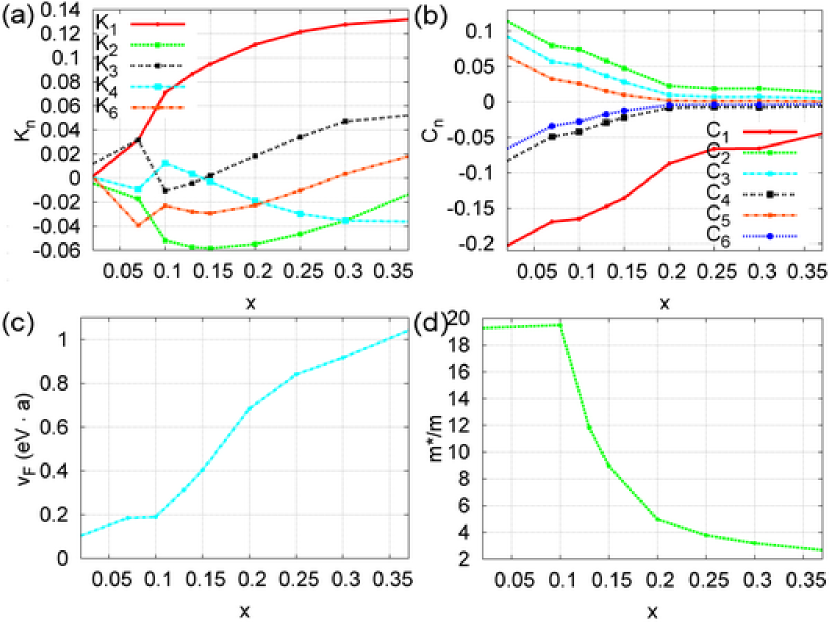
Figure 4: (color online) The same as in Fig.2, but within the model for p-type cuprates without three-site correlated hoppings ($t-t^{\prime}-t^{\prime\prime}-J$ model).

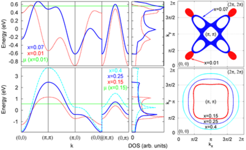
Figure 5: (color online) The same as in Fig.3, but within the model for p-type cuprates without three-site correlated hoppings ($t-t^{\prime}-t^{\prime\prime}-J$ model).

To analyze the effect of the three-site hopping term $H_{3}$ we also calculated the doping dependence of the band structure and FS within the $t-t^{\prime}-t^{\prime\prime}-J$ model. The behavior of the kinematic and the spin-spin correlation functions, presented in Fig. 4, is quite different from that of the $t-t^{\prime}-t^{\prime\prime}-J^{*}$ model. There is only one quantum critical point at $x\approx 0.08$ and the effective mass becomes very large for $x$ approaching zero. For $x>0.1$ the evolution of the FS and density of states near the Fermi level is smooth, without significant changes (see Fig.5). Most part of the difference to the $t-t^{\prime}-t^{\prime\prime}-J^{*}$ model stems from the role of $H_{3}$ in the energy of states near the $(\pi,\pi)$ point, thus determining the topology of the FS and the physics at low doping concentrations (see Fig.1).

IV Results for n-type cuprates

Now let us consider n-type cuprates within the $t-t^{\prime}-t^{\prime\prime}-J^{*}$ model. For NCCO the LDA+GTB calculated parameters are (in eV): $t=-0.50,t^{\prime}=0.02,t^{\prime\prime}=-0.07,J=0.195,J^{\prime}=0.001,J^{\prime\prime}=0.004$.

Figure 6: (color online) The same as in Fig.2, but within the $t-t^{\prime}-t^{\prime\prime}-J^{*}$ model for n-type cuprates.

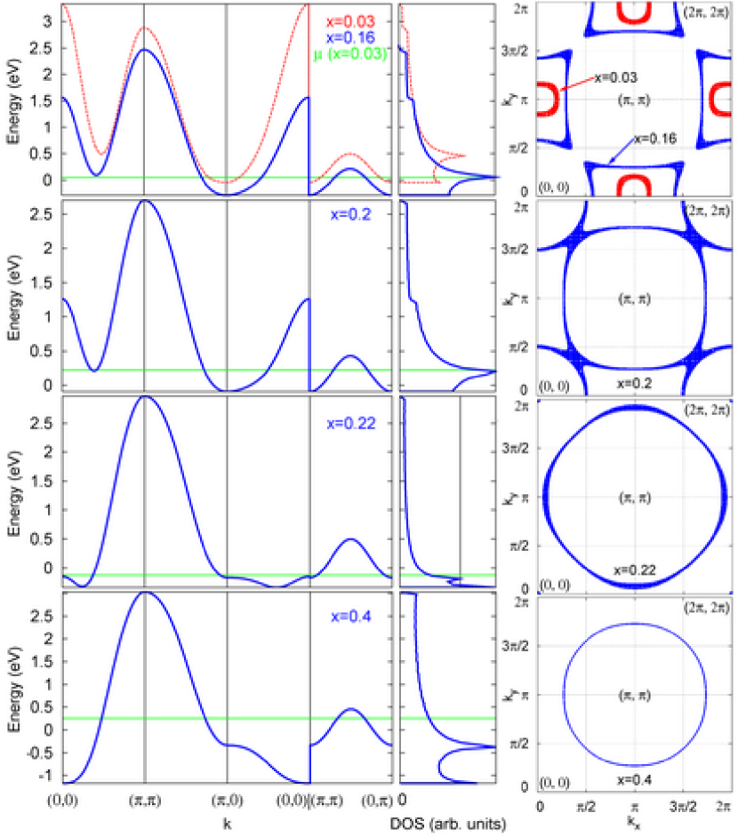
Figure 7: (color online) The same as in Fig.3, but within the $t-t^{\prime}-t^{\prime\prime}-J^{*}$ model for n-type cuprates.

The obtained doping dependence of the kinematic and magnetic correlation functions presented in Fig. 6. There is only one crossover point at $x\approx 0.2$. Also, in contrast to the p-type results, the most important kinematic correlation function on the left of this point is $K_{2}$, rather than $K_{3}$. For $x>0.2$ the system demonstrates Fermi liquid-like behavior with magnitude of kinematic correlation function decreasing with the distance, and small values of the magnetic correlations.

The role of the short range magnetic order and three-site hopping terms in n-type cuprates is similar to that of p-type. In particular, due to the scattering on the magnetic excitations the states near the $(\pi,\pi)$ point pushed above the Fermi level, and the local symmetry around the $(\pi/2,\pi/2)$ points is restored, reminding of the short-range AFM fluctuations (see Fig. 7).

Instead of hole pockets around the $(\pm\pi/2,\pm\pi/2)$ point in p-type, here at low $x$ the electron pockets around $(\pm\pi,0)$ and $(0,\pm\pi)$ points are present. Upon increase of the doping concentration these pockets become larger and merge together at $x=0.2$. For higher concentrations the FS appear to be a large hole-like one, shrinking toward $(\pi,\pi)$ point. Therefore, no other changes in the FS topology other than at $x=0.2$ are present. Referring to the same arguments as in previous section, we claim that in our approach there is only one quantum critical point at $x_{n}=0.2$ in the n-type cuprates. Th non-monotonic change of the effective mass and the nodal Fermi velocity is also present at this concentration, as evident from Fig. 6(c) and (d).

V Discussion and summary

To summarize, we have investigated the doping-dependent evolution of the low-energy excitations for p- and n-type High-$T_{c}$ cuprates in the regime of strong electron correlations within the sequentially derived effective model with the ab initio parameters. We show that due to the changes of the Fermi surface topology with doping the system exhibits drastic change of the low-energy physics. Namely, for p-type cuprates there exist two critical concentrations, $x_{1}\approx 0.15$ and $x_{2}\approx 0.23$. Along the different sides of these concentrations the behavior of the density of states near the Fermi level, of the kinematic and magnetic correlation functions, of the effective mass and the nodal Fermi velocity, is drastically different. This let us speak about crossover, or, taking into account the accompanying FS topology changes, about quantum phase transitions at these quantum critical concentrations.

For n-type cuprates due to the specific FS topology we obtain only one quantum critical concentration, $x_{n}\approx 0.2$.

First of all, we would like to comment on the approximations made in this work. Since we use the perturbation theory with hopping $t$ and exchange $J$ as small parameters, appropriate for the strongly correlated regime, the real part of the corrections to the results obtained will be small to the extent of smallness of the higher powers of $t/E_{ct}$ and $J/E_{ct}$. This will result in the small changes of the band dispersion and in the fine details of the FS, not changing anything qualitatively.

More concerns give the imaginary part of the neglected corrections to the strength operator $\hat{P}(\vec{k},E)$ and to the self-energy $\hat{\Sigma}(\vec{k},E)$ through $\tilde{L}_{\vec{k}}^{\alpha(irr)}$. Application of the equation of motion decoupling method to the Hubbard model with finite quasiparticle lifetime plakida2006 reveals that the results of the mean-field-like approximation is qualitatively correct. Quantitatively, at low doping the imaginary part of the self-energy leads to the hiding of the FS portions above the antiferromagnetic Brillouin zone ($(\pi,0)-(0,\pi)$ line). This results in Fermi arc rather than hole pockets at $x<x_{opt}$ (see Fig. 3). Also, we can compare our results to the numerical methods, namely, to the exact diagonalization studies tohyama2004 . The quasiparticle dispersion of the $t-t^{\prime}-J$ model in Ref. tohyama2004 can be considered as consisting of two bands. For p-type cuprates intensities of the spectral peaks corresponding to the band situated mostly above the Fermi level (in electron representation) are very low. This band is often called a “shadow” band and appears due to the scattering on the short range AFM fluctuations. Notably, our band dispersion from Figs. 3 and 7 reproduce very well the shape of the other, “non-shadow”, band. It is this band where the most part of the spectral weight is residing, thus determining most of the low-energy properties, except for such subtle effects as a so-called “kink” in dispersion zhou2003 .

Also, all renormalizations not included in consideration will change the values of the critical concentrations $x_{1}$, $x_{2}$, and $x_{n}$. Comparing with the results of a more rigorous theory in paper plakida2006 , we expect these values to decrease.

Thus we conclude that our theory captures the most important part of the low-energy physics within the considered (and justified for cuprates) model. This claim is supported by the qualitative agreement with the critical concentrations of crossover observed in the transport experiments ando2004RH ; ando2004 and in the optical experiment gedik2005 ; bontemps2004 ; carbone2006 , and even quantitative agreement of the doping dependence of the nodal Fermi velocity and of the effective mass zhou2003 ; kordyuk2005 ; padilla2005 . Although we use a simple mean-field theory, though strong-coupled, the agreement with the experiments is not surprising since we included all necessary for High-$T_{c}$ copper oxides ingredients. Namely, the short range magnetic order and three-site correlated hoppings. Former is the intrinsic property of the cuprates exhibiting long range AFM order at low $x$, while latter results from the sequential derivation of the low-energy effective model.

- (1) S. Nakamae, K. Behnia, N. Mangkorntong, M. Nohara, H. Takagi, S.J.C. Yates, and N.E. Hussey, Phys. Rev. B 68, 100502(R) (2003).
- (2) K.M. Shen, F. Ronning, D.H. Lu, F. Baumberger, N.J.C. Ingle, W.S. Lee, W. Meevasana, Y. Kohsaka, M. Azuma, M. Takano, H. Takagi, and Z.-X. Shen, Science 307, 901 (2005).
- (3) A. Damascelli, Z. Hussain, and Z.-X. Shen, Rev. Mod. Phys. 75, 473 (2003).
- (4) T. Yoshida, X.J. Zhou, T. Sasagawa, W.L. Yang, P.V. Bogdanov, A. Lanzara, Z. Hussain, T. Mizokawa, A. Fujimori, H. Eisaki, Z.-X. Shen, T. Kakeshita, and S. Uchida, Phys. Rev. Lett. 91, 027001 (2003).
- (5) Y. Ando, Y. Kurita, S. Komiya, S. Ono, and K. Segawa, Phys. Rev. Lett. 92, 197001 (2004).
- (6) Y. Ando, S. Komiya, K. Segawa, S. Ono, and Y. Kurita, Phys. Rev. Lett. 93, 267001 (2004).
- (7) N. Gedik, M. Langner, J. Orenstein, S. Ono, Y. Abe, and Y. Ando, Phys. Rev. Lett. 95, 117005 (2005).
- (8) A.F. Santander-Syro, R.P.S.M. Lobo, N. Bontemps, W. Lopera, D. Girata, Z. Konstantinovic, Z.Z. Li, and H. Raffy, Phys. Rev. B 70, 134504 (2004).
- (9) F. Carbone, A.B. Kuzmenko, H.J.A. Molegraaf, E. van Heumen, V. Lukovac, F. Marsiglio, D. van der Marel, K. Haule, G. Kotliar, H. Berger, S. Courjault, P.H. Kes, and M. Li, Phys. Rev. B 74, 064510 (2006);
- (10) N. Harima, J. Matsuno, and A. Fujimori, Y. Onose, Y. Taguchi, and Y. Tokura, Phys. Rev B 64, 220507(R) (2001).
- (11) X.J. Zhou, T. Yoshida, A. Lanzara, P.V. Bogdanov, S.A. Kellar, K.M. Shen, W.L. Yang, F. Ronning, T. Sasagawa, T. Kakeshita, T. Noda, H. Eisaki, S. Uchida, C.T. Lin, F. Zhou, J.W. Xiong, W.X. Ti, Z.X. Zhao, A. Fujimori, Z. Hussain, and Z.-X. Shen, Nature 423, 398 (2003).
- (12) A.A. Kordyuk, S.V. Borisenko, A. Koitzsch, J. Fink, M. Knupfer, and H. Berger, Phys. Rev B 71, 214513 (2005).
- (13) W.J. Padilla, Y.S. Lee, M. Dumm, G. Blumberg, S. Ono, K. Segawa, S. Komiya, Y. Ando, and D.N. Basov, Phys. Rev. B 72, 060511(R) (2005).
- (14) W.F. Brinkman and T.M. Rice, Phys. Rev. B 2, 4302 (1970).
- (15) M.C. Gutzwiller, Phys. Rev. Lett. 10, 159 (1963); Phys. Rev. B 134A, 923 (1964); Phys. Rev. B 137A, 1726 (1965).
- (16) F. Gebhard, Phys. Rev. B 41, 9452 (1990).
- (17) F. Gebhard, Phys. Rev. B 44, 992 (1991).
- (18) G. Kotliar and A.E. Ruckenstein, Phys. Rev. Lett. 57, 1362 (1986).
- (19) W. Metzner and D. Vollhardt, Phys. Rev. Lett. 62, 324 (1989).
- (20) A. Georges, G. Kotliar, W. Krauth, and M. Rozenberg, Rev. Mod. Phys. 68, 13 (1996).
- (21) M.M. Korshunov, V.A. Gavrichkov, S.G. Ovchinnikov, I.A. Nekrasov, Z.V. Pchelkina, and V.I. Anisimov, Phys. Rev. B 72, 165104 (2005).
- (22) S.G. Ovchinnikov and I.S. Sandalov, Physica C 161, 607 (1989).
- (23) V.A. Gavrichkov, S.G. Ovchinnikov, A.A. Borisov, and E.G. Goryachev, Zh. Eksp. Teor. Fiz. 118, 422 (2000) [JETP 91, 369 (2000)]; V. Gavrichkov, A. Borisov, and S.G. Ovchinnikov, Phys. Rev. B 64, 235124 (2001).
- (24) M.M. Korshunov, S.G. Ovchinnikov, and A.V. Sherman, Phys. Met. Metallogr. 101, Suppl. 1, S6 (2006).
- (25) J.C. Hubbard, Proc. Roy. Soc. London A 277, 237 (1964).
- (26) R.O. Zaitsev, Sov. Phys. JETP 41, 100 (1975).
- (27) Yu. Izumov and B.M. Letfullov, J. Phys.: Condens. Matter 3, 5373 (1991).
- (28) S.G. Ovchinnikov and V.V. Val’kov, Hubbard Operators in the Theory of Strongly Correlated Electrons (Imperial College Press, London, 2004).
- (29) J.C. Hubbard, Proc. Roy. Soc. London A 276, 238 (1963).
- (30) N.M. Plakida, V.Yu. Yushankhai, and I.V. Stasyuk, Physica C 162-164, 787 (1989).
- (31) V.V. Val’kov and D.M. Dzebisashvili, Zh. Eksp. Teor. Fiz. 127, 686 (2005) [JETP 100, 608 (2005)].
- (32) H. Shimahara and S. Takada, J. Phys. Soc. Jpn. 60, 2394 (1991); J. Phys. Soc. Jpn. 61, 989 (1992).
- (33) A. Barabanov and O. Starykh, J. Phys. Soc. Jpn. 61, 704 (1992); A. Barabanov and V. M. Berezovsky, Zh. Eksp. Teor. Fiz. 106, 1156 (1994) [JETP 79, 627 (1994)].
- (34) A. Sherman and M. Schreiber, Phys. Rev. B 65, 134520 (2002).
- (35) A.A. Vladimirov, D. Ile, and N.M. Plakida, Theor. i Mat. Fiz. 145, 240 (2005) [Theor and Meth. Physics 145, 1575 (2005)].
- (36) V.V. Val’kov, T.A. Val’kova, D.M. Dzebisashvili, and S.G. Ovchinnikov, Pis’ma v ZhETF 75, 450 (2002) [JETP Lett. 75, 278 (2002)].
- (37) M.M. Korshunov, S.G. Ovchinnikov, and A.V. Sherman, Pis’ma v ZhETF 80, 45 (2004) [JETP Lett. 80, 39 (2004)].
- (38) I.M. Lifshitz, Sov. Phys. JETP 11, 1130 (1960).
- (39) G.E. Volovik, Acta Phys. Slov. 56, 49 (2006); cond-mat/0601372 (unpublished).
- (40) N.M. Plakida and V.S. Oudovenko, cond-mat/0606557 (unpublished, to appear in Physica C).
- (41) T. Tohyama, Phys. Rev. B 70, 174517 (2004).