From an insulating to a superfluid pair-bond liquid

Abstract

We study an exchange coupled system of itinerant electrons and localized fermion pairs resulting in a resonant pairing formation. This system inherently contains resonating fermion pairs on bonds which lead to a superconducting phase provided that long range phase coherence between their constituents can be established. The prerequisite is that the resonating fermion pairs can become itinerant. This is rendered possible through the emergence of two kinds of bond-fermions: individual and composite fermions made of one individual electron attached to a bound pair on a bond. If the strength of the exchange coupling exceeds a certain value, the superconducting ground state undergoes a quantum phase transition into an insulating pair-bond liquid state. The gap of the superfluid phase thereby goes over continuously into a charge gap of the insulator. The change-over from the superconducting to the insulating phase is accompanied by a corresponding qualitative modification of the dispersion of the two kinds of fermionic excitations. Using a bond operator formalism, we derive the phase diagram of such a scenario together with the elementary excitations characterizing the various phases as a function of the exchange coupling and the temperature.

I Introduction

The evolution of pairing correlations and, the related to it, onset of phase coherence in low dimensional systems is at the center of intense theoretical investigations.phil03 This activity concerns systems such as: (i) high temperature cuprate superconductors with their spin/charge pseudogap phenomenon,lee06 (ii) low temperature superconducting materials which can be driven towards insulating or metallic phases via some extrinsic/intrinsic mechanisms,Jae89 ; Eph96 ; Mas01 (iii) ultra-cold gases of fermionic atoms in the cross-over regime between a BCS state and a Bose-Einstein condensate, controlled by a Feshbach resonanceJoc03 .

In this paper, we shall investigate systems where bosonic resonant pairs form in an ensemble of itinerant uncorrelated fermions. The dynamics of such a boson-fermion exchange coupled system is characterized by two competing processes: A) a local exchange between a localized bound pair of fermions and a pair of itinerant uncorrelated fermions, B) a non-local single particle hopping of the itinerant fermions between nearest neighbor sites.

The exchange between the localized bound pairs (acting as hardcore bosons) and the fermionic itinerant particles creates a local quantum superposition with bonding and antibonding resonant pair configurations given by $|2,i\rangle_{\pm}=\frac{1}{\sqrt{2}}(\rho^{+}_{i}\pm\tau^{+}_{i})|0\rangle$. $\rho^{+}_{i}$ and $\tau^{+}_{i}=c^{\dagger}_{i\uparrow}c^{\dagger}_{i\downarrow}$ denote respectively the creation operators of the two constituents of those local bound pair states, i.e. for hardcore bosons and pairs of itinerant fermions on site $i$. In the atomic limit, these states are separated by an energy difference equal to twice the boson-fermion exchange coupling, with the bonding state being energetically favorable.

The local quantum structure of the bonding configuration, responsible for inducing local resonant pairing among the fermions, has at the same time a hindering effect in establishing a long range superconducting spatial correlations of such resonating pairs.

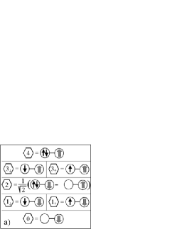
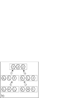
Figure 1: The a) panel provides the description of the possible configurations on the single bond (hexagon). The bold arrow is associated with the pseudospin for the original localized bound pairs. The b) panel indicates the possible mechanisms of dissociation starting from a representative string of three neighbor bonding bosons. The successive two steps for that are: i) the formation of two kinds of pairs, $1$ involving single individual fermions on a bond and the other made up with charges $3$ due to individual fermions attached with a bound pair on a bond and subsequently ii) the bond fermions pairing up and resonating with the bond-holes and the double-pairs-bonds.

Spatial correlations between the bonding/antibonding pairs are built up via other bosonic and fermionic bond configurations which form the local Hilbert space which has a very rich structure (see Fig. 1a). There are two fermion-like configurations which result from attaching to the vacuum state one individual fermion (configuration ${}^{\prime\prime}1_{\sigma}^{\prime\prime}$), respectively such an individual fermion together with a localized bosonic bound fermion pair (configuration ${}^{\prime\prime}3_{\sigma}^{\prime\prime}$). Moreover, in this bond Hilbert space we have completely empty bonds - bond-holes ${}^{\prime\prime}0^{\prime\prime}$ - and completely filled ones - double-pair-bond states ${}^{\prime\prime}4^{\prime\prime}$. The fermionic objects are itinerant. Their mobility is due to the creation/annihilation of bonding (respectively anti-bonding) and bond-holes (respectively double-paired bonds).

Our main aim in this study is to show that, due to the internal degrees of freedom of the two components (localized hardcore bosons and itinerant fermions), there are two distinct energy scales in this problem: one controlled by the dynamics of the bonding pairs and one by the dynamics of the bond-holes and double-paired bonds (see Fig. 1b). Depending on the ratio between the exchange coupling strength and the hopping amplitude, the dynamics of the two kinds of fermionic excitations can lead to either i) their pairing up in a superconducting state where simultaneously a coherent state with bonding pairs, bond-holes and double-paired bonds occurs, or ii) an insulating state with coherent bonding pairs and with zero amplitude of the bond-holes/double-paired bonds (see Fig.1b).

The presence of bonding pairs does not guarantee by itself the occurrence of long range superconducting correlations between their paired constituents. They have to dissociate in order to induce a superconducting state. This process of dissociation involves two possible channels for the dynamics of this resonant pairing scenario (see Fig.1b): i) the single fermions and the composite ones (constituted of a fermion-boson pair) hybridize and their itinerancy sustains a coherent liquid of bonding pairs, ii) the two kinds of fermions pair up and resonate with the bond-holes and double-paired bonds and via that result in a superconducting state.

Within this context, our target is the following: I) determine the evolution of the superconducting state into an insulating state, both quantum and thermally driven, II) analyze the nature of the excitation spectrum as a function of the exchange coupling.

The outline of the paper is the following: in Sec II we present the scenario for resonant pairing, on the basis of three examples actively studied in the literature. In Sec. III we sketch the bond operator formalism and adapt it to the boson-fermion problem. Sec. IV is devoted to the derivation of the phase diagram as a function of exchange coupling and temperature features. In Sec. V, we present the evolution of the excitation spectrum as one tunes the ground state from a superconductor to an insulator. The last section VI is reserved for the summary, conclusions and outlook.

II The Boson-Fermion scenario

There is a variety of different physical systems where fairly localized bound states are quasi degenerate with itinerant states of their constituents. They can be paraphrased in terms of a two-component system composed of localized bosonic pair states, itinerant fermionic quasi-particles and a local exchange interaction between the two. Such a scenario is described by the so called boson-fermion model (BFM) Hamiltonian

$$H =(D-\mu)\sum_{i\sigma}c_{i\sigma}^{\dagger}c_{i\sigma}^{\phantom{\dagger}}+(\Delta_{B}-2\mu)\sum_{i}(\rho_{i}^{z}+\frac{1}{2})$$ (1)

$$- \sum_{i\neq j,\>\sigma}t_{ij}(c_{i\sigma}^{\dagger}c_{j\sigma}^{\phantom{\dagger}}+H.c.)+g\sum_{i}\left(\rho^{+}_{i}\tau^{-}_{i}+\rho^{-}_{i}\tau^{+}_{i}\right),$$

where $g$ is the strength of the exchange interaction and $t$ the hopping integral for the itinerant fermions, which is assumed here to be different from zero only for nearest neighbor sites. The band half-width (which will serve as energy unit) is $D=zt$, $z$ being the coordination number of the underlying lattice. The energy of the bound fermion pairs is denoted by $\Delta_{B}$. The number of the ensemble of bosons and fermions being conserved, $n_{tot}=n_{F\uparrow}+n_{F\downarrow}+2n_{B}$, implies a common chemical potential $\mu$ for both subsystems. $n_{B}$ and $n_{F\sigma}$ are the occupation numbers per site of the hard core-bosons and of the fermions with spin $\sigma=\uparrow,\downarrow$. In the present study, we restrict ourselves to the analysis for the fully symmetric half-filled band case ( $\Delta_{B}\equiv 0$), which in such a two-component system means $n_{tot}=2$. The annihilation (creation) operators for the fermions with a spin $\sigma$ at a certain site $i$ are given by $c^{(\dagger)}_{i\sigma}$, those for the hard-core bosonic fermionic bound pairs by the pseudospin-$\frac{1}{2}$ $\rho^{\pm}_{i}$ and similarly those for the pairs of itinerant uncorrelated fermions by $\tau^{+}_{i}=c_{i\uparrow}^{\dagger}c_{i\downarrow}^{\dagger}$, $\tau^{-}=c_{i\downarrow}c_{i\uparrow}$.

This model was introduced originally by one of us (JR) in an attempt to capture the salient features of polaronic systems in the intermediate coupling regime between adiabaticity and anti-adiabaticity, but has turned out subsequently to be of much more general relevance and applicability. Among others, such a scenario has led to the prediction of the charge pseudogap features in the high $T_{c}$ cuprate superconductorsRanninger-95 , without having to invoke any particular microscopic mechanism for that. We shall discuss briefly three representative examples where such a scenario seems to be relevant.

(i) In a system with strong local electron-lattice coupling we have the formation of small polaronic charge carriers, which in general will exist in form of localized bipolarons. If their binding energy exceeds the bandwidth of the itinerant electrons in an undeformed lattice, this can give rise to bipolaronic superconductivity - an extremely fragile state of a phase fluctuation controlled condensate of bosonic tightly bound electron pairs - whose existence in real materials has yet to be experimentally verified. However, if the binding energy of such localized bipolarons is such that it overlaps with the continuum of the bare electron band states, this will result in an exchange between such bound pairs and pairs of uncorrelated itinerant electrons close to the chemical potential. The microscopic mechanism for that exchange arises from large quantum fluctuations of the lattice displacements in the immediate vicinity of the charge carriers. Such local lattice displacements fluctuate between essentially undeformed and much deformed lattice environments which, as a result, periodically capture and release electron pairs on small local cluster (acting as effective sites on a lattice) made up of atoms and their associated ligand environementsRanninger-Romano-06 .

(ii) In a system with strong local electronic correlations, as described by the Hubbard model close to the half-filled band case, hole pairing occurs on small plaquette clusters.White-Scalapino-97 This, coexisting with triplet spin pairs, destroys the antiferromagnetic long range order, giving rise to a spin liquid state made out of singlet hole pairs, which conceivably can condense into a superfluid state.Anderson-87 One of the possible mechanism for that is the hopping of the singlet hole pairs between neighboring clusters. A more efficient way to get this condition is by exchanging the local bound hole pairs on a plaquette with single holes on neighboring plaquettes. This mechanism results in an effective exchange coupling between bosonic bound hole pairs and pairs of uncorrelated fermionic holes on adjacent plaquettes, which at the end assure the itinerancy in the system. Such a scenario has been analyzed on the basis of a kind of real space renormalization group technique, where the initial Hubbard model can be rephrased in terms of an effective BFM, albeit with additional terms carrying the information of the underlying antiferromagnetic short range interaction.Altman-Auerbach-02

(iii) In a system with an optically trapped gas of ultracold fermionic atoms (studied in connection with the cross-over between a BCS state of weakly interacting fermionic atoms and a Bose-Einstein condensation of tightly bound states of them) one can monitor the strength of the interaction between those fermions - sweeping it from a repulsive to an attractive interaction - via a so called Feshbach resonance mechanismFeshbach-58 ; Timmermans-99 - under the effect of a magnetic field. This mechanism is based on binary collision processes in which the inter-atomic interaction depends on the electronic spin configuration of the pair. For an overall electronic spin triplet state (avoiding the Coulomb repulsion) this leads to a weakly bound state, while a singlet configuration leads to scattering states. Two incident atoms in a singlet configuration can enter into a resonance with such a weakly bound triplet configuration molecular state when their respective energies are close to each other. This is achieved by flipping the electron spin on one of the two atoms via a hyperfine interaction, thus acquiring the necessary triplet configuration to bind them momentarily into a pair. By applying a magnetic field during such binary scattering processes one can change the relative position of the energy levels of the two electron spin configuration and thus enter in a resonance regime where they are quasi degenerate. Such a situation can be then described by a phenomenological model such as the BFM.

III Bond operator representation

To study the scenario for resonant pairing, sketched above, by explicitly taking into account the interplay between the bosonic bonding pairs and the processes linking them to the single particle fermionic entities, we make use of the bond operator formalism and adapt it to the present BFM system. This approach turns out to be particularly appropriate in treating situations where there is a natural pairing in form of dimers in the ground state, which is either imposed by the Hamiltonian (as in our case) or by a spontaneous symmetry breaking. The bond operator theory has been successfully designed and applied in different contexts such as for antiferromagnetsSach90 ; Chub91 , spin-ladderGopa94 , doped antiferromagnetsPark01 , bilayer quantum HallDeml99 , and Kondo lattice systemsJure01 .

Introducing the bond operator formalism for the BFM, we start from a bond on each lattice site being made up of fermionic and bosonic configurations and then express the original fermionic and bosonic operators $c^{(\dagger)}_{i\sigma},\rho^{\pm}_{i},\tau^{\pm}_{i}$ in terms of the new basis. Concerning a single local bond, one has eight possible configurations to start with. Similar to the case of a spin insulator, where one is introducing the singlet and triplet boson operator, here we have four boson operators that describe two-particle configurations in form of bonding-bonds and antibonding-bonds and zero- as well as four-particle configurations in form of hole-bonds and double-paired-bonds. The two-particle bonding and antibonding configurations can be expressed in terms of pseudospin-$\frac{1}{2}$ operators $\tau^{+}_{i},\rho^{+}_{i}$ for the uncorrelated fermions and the tightly bound ones. The zero- and four-particle configurations are described by $|0\rangle$ and $\rho^{+}_{i}\tau^{+}_{i}|0\rangle$ respectively. We thus have to consider four bond boson operators $b^{(\dagger)}$, $a^{(\dagger)}$, $f^{(\dagger)}$, and $d^{(\dagger)}$ (see Fig. 1a) with

$$b^{\dagger}|v\rangle = \frac{1}{\sqrt{2}}\left[\rho^{+}-\tau^{+}\right]|0\rangle$$

$$a^{\dagger}|v\rangle = \frac{1}{\sqrt{2}}\left[\rho^{+}+\tau^{+}\right]|0\rangle$$

$$f^{\dagger}|v\rangle = \rho^{+}\tau^{+}|0\rangle$$

$$d^{\dagger}|v\rangle = |0\rangle.$$ (2)

$|0\rangle=|0_{f}\rangle\otimes|0_{b}\rangle$ denotes the boson-fermion vacuum, i.e., the state with no fermions ($c_{\sigma}|0\rangle=0$) and no bosons present ($\rho^{-}|0\rangle=0$). $|v\rangle$ designates a corresponding new vacuum state in which neither bond-bosons nor bond-fermions are present. The remaining configurations are four bond-fermion operators describing individual fermionic states and states where such fermions are attached to a boson on a particular bond:

$$h_{\sigma}^{\dagger}|v\rangle = c_{\sigma}^{\dagger}|0\rangle$$

$$s_{\sigma}^{\dagger}|v\rangle = \rho^{+}c_{\sigma}^{\dagger}|0\rangle\,.$$ (3)

The operators $h^{(\dagger)},s^{(\dagger)}$ obey the canonical fermion commutation relations, while $d^{(\dagger)},f^{(\dagger)},b^{(\dagger)},a^{(\dagger)}$ have boson commutation rules. In this representation, the total number of states in the Hilbert space of these four bond bosons and four bond fermions is much larger than the eight configurations allowed by the BFM. To limit the kinematics to the physical subspace one has to impose the closure relation on the bond given by the constraint:

$$f^{\dagger}f+\sum_{\sigma}s_{\sigma}^{\dagger}s_{\sigma}+b^{\dagger}b+a^{\dagger}a+\sum_{\sigma}h_{\sigma}^{\dagger}h_{\sigma}+d^{\dagger}d=\mathrm{1}\,.$$ (4)

In the subspace limited by the relation (Eq. 4), one then derives the expressions for the original fermion and hard-core bosonic operators in terms of bond operators.

Let us first consider the fermion creation operator with spin $\sigma$. Making use of the closure relation (Eq. 4) and considering all possible transitions induced by the single particle fermionic operator between the different bond quantum configurations, we obtain the following expression:

$$c_{\sigma}^{\dagger}=p_{\sigma}f^{\dagger}s_{-\sigma}+\frac{1}{\sqrt{2}}s_{\sigma}^{\dagger}\left(b+a\right)+\frac{p_{\sigma}}{\sqrt{2}}\left(a^{\dagger}-b^{\dagger}\right)h_{-\sigma}+h_{\sigma}^{\dagger}d\,,$$ (5)

where $p_{\sigma}=(+1,-1)$ for $\sigma=(\uparrow,\downarrow)$. In a similar way one obtains for the creation operator of a hard core boson:

$$\rho^{+}=\frac{1}{\sqrt{2}}f^{\dagger}(a-b)+\sum_{\sigma}s_{\sigma}^{\dagger}h_{\sigma}+\frac{1}{\sqrt{2}}(b^{\dagger}+a^{\dagger})d\,.$$ (6)

This, subsequently leads to the following expressions for the density operators for the bosons and fermions:

$$\rho^{+}\rho^{-} = \frac{1}{2}(a^{\dagger}a+b^{\dagger}b+a^{\dagger}b+b^{\dagger}a)+f^{\dagger}f+\sum_{\sigma}s_{\sigma}^{\dagger}s_{\sigma}$$

$$c_{\sigma}^{\dagger}c_{\sigma} = \frac{1}{2}(a^{\dagger}a+b^{\dagger}b-a^{\dagger}b-b^{\dagger}a)+f^{\dagger}f+\left(s_{\sigma}^{\dagger}s_{\sigma}+h_{\sigma}^{\dagger}h_{\sigma}\right).\,$$

Finally, the expression for the pair exchange on the bond between the initial fermions and bosons reduces in the new representation to just the difference between the number of bonding and antibonding bosons, that is:

$$\rho^{+}\tau^{-}+\tau^{+}\rho^{-}=a^{\dagger}a-b^{\dagger}b\,.$$ (8)

IV Mean-field phase diagram

Let us now apply the bond operator method to study the spectral properties of the BFM, in conjunction with its various possible phases. We proceed by looking for solutions where the bosons associated with the bonding-bonds $b^{(\dagger)}$, antibonding-bonds $a^{(\dagger)}$, the bond holes $d^{(\dagger)}$, and double-paired-bonds $f^{(\dagger)}$ are condensed. This means that in the Hamiltonian, Eq.1, after having transformed the original fermion and boson operators into the new bond operators, one is decoupling the quartic terms in a way such that the expectation value of the linear and bilinear bond boson operators have a non-zero amplitude, $\langle o\rangle=\bar{o}$, with $\bar{o}=\bar{b},\bar{a},\bar{f},\bar{d}$. The coherent state which then emerges in the most general case has the following local structure:

$$|\psi_{c}\rangle=(u_{v}+u_{b}b^{\dagger}+u_{a}a^{\dagger}+u_{d}d^{\dagger}+u_{f}f^{\dagger})|v\rangle,$$ (9)

where the finite amplitudes of the various coefficients $u$ are related to the condensate of the corresponding bosonic degrees of freedom. Let us, at this point, make some general observations related to the structure of the Hamiltonian in such a bond operator representation. The $b$-bond bosons are always condensed at zero temperature ($\bar{b}\neq 0$), due to the local exchange and the hopping induced processes related to the creation of $d$-bond bosons and $s$, $h$ bond fermions. Moreover, the $d$-bond bosons condense only if simultaneously the $f$-bond bosons condense and in our present analysis concentrating on the particle-hole symmetric half-filled band case, we have ($\bar{d}=\bar{f}\neq 0$). In the present mean field approach the $a$-bond bosons have gapped excitations due to the exchange splitting with respect to the $b$-bond bosons and hence do not contribute to a coherent state in the lowest energy configuration.

Let us now examine the possible solutions at zero temperature as a function of the exchange coupling $g$. Our main objective is to show how, above a critical value of the ratio $g/D$, the system passes from a superconducting state with simultaneous coherence of $b$-bond bosons and the $d$-bond as well as $f$-bond bosons, to an insulating state where only the $b$-bond bosons are condensed.

Before going into the details about such a calculation and the results, let us point out certain aspects of the emerging bond boson-fermion dynamics which can be envisaged on simple and quite general physical grounds. As mentioned before, the $b$-bond bosons are always in a coherent state at zero temperature, due the local exchange and the quantum processes of double creation and annihilation of nearest neighbor $b$-bond bosons. Hence, the U(1) symmetry associated to the number conservation of the $b$-bond bosons is generally broken in the entire regime of couplings $g$. In the weak coupling regime, $b$-bond bosons have a large dispersion which, together with coherent $d$-bond and $f$-bond bosons, leads to a superconducting state. In the intermediate/strong coupling regime, the $b$ bosons become more populated, which is caused by an increased local binding energy. This increase in the $b$, $d$ boson occupation leads to a decrease of the $s$- and $h$-bond fermion densities, which ultimately causes a reduction of the $b$ boson dispersion. Once the $d$- and $f$-bond bosons are no longer condensed, the coherence of the $b$-bond bosons is built up via processes described by the terms $b_{i}b_{j}s^{\dagger}_{i\sigma}h^{\dagger}_{j\bar{\sigma}}$($b^{\dagger}_{i}b^{\dagger}_{j}s_{i\sigma}h_{j\bar{\sigma}}$) in the Hamiltonian.

Let us now consider the physics sketched above in terms of a mean-field analysis of the BFM. After performing the corresponding decoupling procedure, the Hamiltonian can be separated into three main parts:

$$H=H_{t}+H_{ex}+H_{0},$$ (10)

where $H_{t}$ is the hopping term, $H_{ex}$ the local pair exchange, and $H_{0}$ a term including the contributions coming from bond bosons in the chemical potential term and the constraint. Here, the constraint is treated in an approximative way, where the corresponding Lagrange multiplier is taken as spatially homogeneous and which has to be determined variationally as a saddle point solution of the total free energy. In our mean-field approximation, we rewrite the first part of Eq. 10 in a compact way by introducing the vector operator $D_{k}=(s_{k,\uparrow},s_{-k,\downarrow}^{\dagger},h_{k,\uparrow},h_{-k,\downarrow}^{\dagger})$ and its hermitian conjugate $D_{k}^{\dagger}=(s_{k,\uparrow}^{\dagger},s_{-k,\downarrow},h_{k,\uparrow}^{\dagger},h_{-k,\downarrow})$ in terms of the Fourier representation for the bond fermions. The single-particle excitations are then determined by the following mean field Hamiltonian:

$$H_{t}=\sum_{k}D_{k}^{\dagger}\,\hat{U}_{k}\,D_{k}+c,$$ (11)

where $c=2\lambda-4\mu$ is a constant which arises in the process of ordering of the various bond fermionic operators. The 4x4 matrix $\hat{U}_{k}$ is given by:

$$\left[\begin{tabular}[]{ccccccc}$\gamma^{s}_{k}$&\thinspace&$\Delta^{s}_{k}$ \thinspace&$\gamma^{\bar{s}h}_{k}$&\thinspace&$\gamma^{\bar{s}\bar{h}}_{k}$\\ &&&&&&\\ $\Delta^{s}_{k}$&\thinspace&$-\gamma^{s}_{k}$ \thinspace&$\gamma^{{s}h}_{k}$&\thinspace&$-\gamma^{\bar{s}h}_{k}$\\ &&&&&&\\ $\gamma^{\bar{s}h}_{k}$&\thinspace&$\gamma^{sh}_{k}$ \thinspace&$\gamma^{h}_{k}$&\thinspace&$\Delta^{h}_{k}$\\ &&&&&&\\ $\gamma^{\bar{s}\bar{h}}_{k}$&\thinspace&$-\gamma^{\bar{s}h}_{k}$ \thinspace&$\Delta^{h}_{k}$&\thinspace&$-\gamma^{h}_{k}$\end{tabular}\right]$$

$\epsilon_{k}=-t\sum_{\delta}\exp[ik\cdot{\delta}]$ is the free particle spectrum of the original fermions, with $\delta$ designating the lattice vectors linking nearest neighbor sites. $\gamma^{s}_{k}=\epsilon_{k}[0.5*(b+a)^{2}-f^{2}]-3\mu+\lambda$, $\gamma^{h}_{k}=\epsilon_{k}[d^{2}-0.5*(b-a)^{2}]-\mu+\lambda$ are the single particle energy spectra for the $s$ and $h$ fermions. $\gamma^{\bar{s}h}_{k}=\frac{\epsilon_{k}}{\sqrt{2}}\{[(b+a)d]-[\left(a-b\right)f]\}$ and $\gamma^{\bar{s}\bar{h}}=\epsilon_{k}[(f\,d)\,+\frac{1}{2}\left(a^{2}-b^{2}\right)]$ are the particle/hole and particle/particle hybridization factors between the $s$- and $h$-bond fermions. The pairing amplitudes for the $s$- and $h$-bond fermions are $\Delta^{s}_{k}=\epsilon_{k}\sqrt{2}[f(b+a)]$ and $\Delta^{h}_{k}=\epsilon_{k}\sqrt{2}[d(a-b)]$, respectively.

Let us next investigate how the effective hopping of the $s,h$-bond fermions depends on the amplitude and the density of the condensed bosons. As one can see by inspection of the matrix $\hat{U}_{k}$, the processes linked to the fermionic degrees of freedom are strongly renormalized by the strength of the condensed $b$-bond bosons. Concerning the dispersion of the $s,h$-bond fermions, one can see that the contribution of the density of the $d,f$-bond bosons counteracts that of the $b$-bond bosons. The strength of the pairing amplitude being proportional to the product of the $b$-bond and $d,f$-bond boson condensate amplitudes, indicates the need of having both types of bond bosons condensed in a state where the $s,h$-bond fermions are paired up. The hybridization between the $s$- and $h$-bond fermions manifests itself in both, the particle/particle and in the particle/hole channel. While the amplitude $\gamma^{\bar{s}h}_{k}$ of the $s-h$ hybridization is linearly linked to the $b$-bond and $d,f$-bond boson condensate, the processes related to the particle/particle mixture depend on the effective density of the $b$-bond bosons as well as the $d,f$-bond bosons. All those processes compete with each other, resulting in either a superconducting or an insulating state, depending on the value of $g/D$.

Let us next examine the exchange and the local contributions of the BFM, which after a corresponding mean-field decoupling are given by:

$$H_{ex}= L\,g(\bar{a}^{2}-\bar{b}^{2})$$

$$H_{0}= -L\,\mu[4\bar{f}^{2}+2(\bar{b}^{2}+\bar{a}^{2})]+$$ (12)

$$L\,\lambda[\bar{f}^{2}+\bar{b}^{2}+\bar{a}^{2}+\bar{d}^{2}-1]$$

and where $L$ indicates the total number of bonds. The procedure of the present analysis is to look for a saddle point solution of the total free energy with respect to the bond boson amplitudes and the Lagrange multiplier for the constraint. The free energy is obtained after performing a Bogoliubov rotation of the $s$, $h$-bond boson operators in the $H_{t}$ term, bringing it into the diagonal form:

$$H_{t}=\sum_{k}E_{\alpha\,,k}\,\eta_{\alpha,k}^{\dagger}\,\,\eta_{\alpha,k}.$$ (13)

$E_{\alpha\,,k}$ ($\alpha=1,..,4$) are the eigen-energies of the various Bogoliubov quasi-particles $\eta_{\alpha,k}^{\dagger}$($\eta_{\alpha,k}$), obtained by diagonalizing the matrix $\hat{U}_{k}$. They result from a unitary transformation of the original fermions and thus have the same commutations relations as $D_{k}^{\dagger}$($D_{k}$). The free energy is then given by the following expression:

$$F = -\frac{1}{\beta}\frac{1}{L}\sum_{k}\sum_{i=1,..4}\ln[2\cosh(\frac{\beta}{2}E_{i,k})]+E_{0}$$

$$E_{0} = g(\bar{a}^{2}-\bar{b}^{2})-\mu[4\bar{f}^{2}+2(\bar{b}^{2}+\bar{a}^{2})]+$$ (14)

$$\lambda[\bar{f}^{2}+\bar{b}^{2}+\bar{a}^{2}+\bar{d}^{2}-1]\,$$

with $\beta=1/(k_{B}T)$.

The saddle point solutions for the bond bosons together with the Lagrange multiplier are obtained variationally by requiring the following extremal conditions:

$$\frac{\partial F}{\partial\lambda}=0$$

$$\frac{\partial F}{\partial\bar{a}}=\frac{\partial F}{\partial\bar{b}}=\frac{\partial F}{\partial\bar{d}}=\frac{\partial F}{\partial\bar{f}}=0$$ (15)

together with the chemical potential being fixed via the relation $n_{tot}=-\frac{\partial F}{\partial\mu}$.

In Fig.2, we report the evolution of the amplitude for the condensed $b$-bond bosons at zero temperature as a function of $g/D$. Throughout this paper we use a 2-dimensional fermionic tight binding spectrum $\epsilon_{k}=-(D/2)(\cos[k_{x}]+\cos[k_{y}])$ for the original fermions. The self-consistent solutions of the non-linear Eqs. 15 yield a zero amplitude for the $a$-bond bosons, as anticipated above, and an equal amplitude for the $d$- and $f$-bond bosons. The latter is a consequence of the particle-hole symmetric case considered here. We also find a clear separation between two distinct regions as the exchange coupling is varied. Below a critical $g_{crit}/D\sim 0.4$ the system allows a finite condensation of the $d,f$-bond and the $b$-bond bosons, which signifies a superconducting state. Yet, upon increasing the exchange coupling, the amplitude of the $d,f$-bond bosons gets reduced, until above $g_{crit}$, the ground state does not contain anymore any $d$-bond bosons. The transition is continuous, merely showing a change of slope in the behavior of $\bar{b}$.

A particular feature of this mean field analysis at $T=0$ is that the order parameter $\bar{d}$, controlling the superconducting phase, has a finite value as soon as the boson-fermion exchange mechanism is switched on, i.e., for $g/D\neq 0$ however small it might be. In the limiting case were the exchange coupling is zero, the superconducting solution disappears because then $b$-bond and $a$-bond bosons are equally populated. Such a degeneracy is removed as soon as the exchange coupling is different from zero. The $b$-bond bosons are now being able to condense while $a$-bond bosons will not. Thus, in the present mean field treatment the system finds the solution with a finite amplitude for the $b$-bond and $d,f$-bond bosons as soon as the exchange is switched on at a non-zero value. The size of the $b$-bond boson amplitude is then related to the constraint and via that to the total filling under consideration.

At this point we would like to make a few remarks on the weak coupling regime. Since the mean-field analysis is based on a local ansatz for the saddle point solution, we do expect that the present approach is best suited for the strong-coupling limit. In the weak coupling limit such a scheme of approximation is not completely satisfactory. In that regime, the dynamics of the bond bosons and their delocalized behavior have to be taken into account in order to properly consider their phase and amplitude fluctuations and the related to it consequences on the fermionic subsystem. The bosonic fluctuations should renormalize down to zero the value of the critical temperature in this small coupling region. The finite amplitude of T_c at $g/D\sim 0$, obtained in our present mean-field analysis, indicates that the pairing formation is driven by kinetics and an overestimation of the phase locking with respect to the amplitude fluctuations of the bond boson order parameter occurs. This physically unsatisfactory feature is corrected by including the competition between the phase and amplitude dynamics, as we have done in a recent work where an effective phase action has been derived after integrating out the fermionic degrees of freedom (see insert in Fig. 3).Cuo05 We do believe that, even in the weak coupling regime, a BCS type of superconductivity should not occur since the charge dynamics intrinsically involves the two types of $s-$ and $h-$ bond fermions. A direct decoupling of the exchange interaction in the starting representation of the BFM would hence not be justified as the hard core bosons are localized fields and thus in principle cannot have a phase coherent amplitude in the transverse mode. In an attempt to include the mobility of the bosons, in a self-consistent perturbative (weak-coupling limit) approach, it has been shown that already above the superconducting transition temperature one gets, apart from the regular free band spectrum, two rather dispersion-less branches.Ran96 As we will see below, such an excitation spectrum resembles that obtained in the present approximation. Hence, within our saddle point solution qualitatively correct features can be recovered even in the weak-coupling regime.

Figure 2: Phase diagram at zero temperature as given by the evolution of the bonding bosons and bond hole amplitude. SC and I stands for a superconducting and insulating state respectively.

Concerning the dynamics of the bosons, we should make a few remarks about the possible nature and the character of the bosonic excitations near the quantum phase transition between the superconducting and the insulating state - in a frame that is beyond our present approximative mean field scheme of investigation. Focusing on the dynamics on the insulating side, we observe that the fermionic excitations are gapped, while the $b$-bond bosons may have low energy gapless excitations resulting from their itinerancy. However, such excitations are not ${}^{\prime\prime}charged^{\prime\prime}$, i.e., capable of creating a pair of fermions, or a localized boson, since that would require at the same time the presence of both $b$-bond as well as $d,f$-bond bosons. Hence, two scenarios are possible as $g/D$ is increased: i) the $d,f$-bond boson coherence and their density go to zero simultaneously, ii) the phase coherence of the $d$-bond bosons drops to zero before their density vanishes. Case i) corresponds to a direct transition between the superconducting to an insulating configuration with coherent $b$-bond bosons. Case ii) allows to have an intermediate state, where a finite density of $d,f$-bond bosons occurs in a state that is not condensed. In this case, the current can be carried directly by the mobile $b$-bond and $d,f$-bond bosons, and the presence of these low energy excitations can induce a metallic-like state. This regime is quite exotic, since the effect of the $a$-bond bosons in activating itinerant pairs can induce a gap in the bosonic sector and, in this way, result again in an insulating state. The picture that finally could emerge is one of a system that undergoes first a transition from a superconductor to a metallic-like phase (built out of a state where incoherent itinerant $b$-bond and $d,f$-bond bosons are present and which ultimately transits to an insulating state where, (driven by the exchange coupling and due to the constraint) there exist only condensed $b$-bond bosons and no condensed $d,f$-bond bosons.

Figure 3: Phase diagram at finite temperature as a function of $g/D$ as given by the evolution of the $b$-bond boson and $d$-bond boson amplitude. SC, BP and N stands for a superconducting, bond coherent boson phase, and normal state, respectively. The insert shows the evolution of the critical superconducting temperature as obtained within a path-integral approach.Cuo05

Let us now analyze the behavior of the two coherent states as a function of temperature (see Fig. 3). In the structure of the phase diagram one notices three regions that are reminiscent of the configurations found at zero temperature. The superconducting state (SC) is characterized by a non-zero amplitude for the $b$- as well as $d,f$-bond bosons, the BP (bond phase) by condensed $b$-bond bosons but a zero amplitude of the $d,f$-bond bosons, while in the normal (N) high temperature phase none of the bond bosons are condensed. As a consequence of the competition between the $b$-bond and $d,f$-bond boson condensation, one has two regimes depending on the exchange coupling in the region where SC is stable at zero temperature. For values of the exchange coupling below $g^{*}/D=0.125$, the SC critical temperature ($T_{bd}$) and that associated with the $b$-bond boson condensation ($T_{b}$) are very close in amplitude so that there occurs an almost direct transition from the SC to the N phase. In this limit, the scales of energy that controls the $b$-bond and $d,f$-bond dynamics are comparable. Going to a larger exchange couplings ($g>g^{*}$), the characteristic temperature marking the onset of SC is reduced due to the increased population of the $b$-bond bosons. But contrary to that, $T_{b}$ grows almost linearly with the coupling. Thus, outside the quantum phase transition region there occurs a large region in parameter space, where the system is not superconducting but is still characterized by a coherent state of $b$-bond bosons.

V Evolution of the charge gap and of the spectral function from the superconducting to the insulating region

In this section we analyze the excitation spectra both for the $s$- and $h$-bond fermions and for the original $c$ fermions. We shall focus on the evolution of the spectral function when moving from the superconducting to the insulating region in the phase diagram. In the previous section, we have constructed the vector $D_{k}$, with $D_{k,i}$ denoting its $i-th$ component. Due to its structure, the time dependent correlation function for the vector $D_{k}$ contains the information for the matrix Green’s function both for the diagonal and the off-diagonal anomalous part of the $s$- and $h$-bond bosons. Using the relation which connects the $s$- and $h$-bond-fermions and the $b$-bond bosons with the original $c$ type fermions, we are able to extract the spectral function for the original fermions. For that, it is convenient to introduce the following time dependent correlation function:

$$G_{k}^{ij}(\tau)=-\langle T\left(D_{k,i}(\tau)D_{k,j}^{\dagger}(0)\right)\rangle$$ (16)

where $i,j=1,..,4$ and $\tau$ is the Matsubara imaginary time, $T$ the usual time ordering operator, and $\langle...\rangle$ indicates the average at finite temperature. Due to the bilinear structure of the Hamiltonian, we readily determine the Green function via its equation of motion. We thus obtain the following expression in matrix notation:

$$\hat{G}_{k}(\omega_{n})=(i\omega_{n}\mathbf{1}-\hat{U}^{k})^{-1}\,.$$ (17)

Figure 4: Zero temperature evolution of the charge gap associated with the excitation of a $c$ fermion as a function of the exchange coupling.

The Green’s function for the original $c$ operators, is consequently a linear combination of the contributions of the different components $G_{k}^{ij}(\tau)$ which are weighted by the various amplitudes of the condensed $b$-bond bosons. This is because of our mean field approach where in the expression for the fermionic $c$ operators, Eq. (5), the various boson operators are replaced by their mean field averages, i.e.,

$$c_{i\sigma}^{\dagger} = p_{\sigma}\bar{f}s_{i\bar{\sigma}}+\frac{1}{\sqrt{2}}s_{i\sigma}^{\dagger}\left(\bar{b}+\bar{a}\right)+\frac{p_{\sigma}}{\sqrt{2}}\left(\bar{a}-\bar{b}\right)h_{i\bar{\sigma}}+h_{i\sigma}^{\dagger}\bar{d}$$

$$c_{i\sigma} = p_{\sigma}\bar{f}s_{i\bar{\sigma}}^{\dagger}+\frac{1}{\sqrt{2}}s_{i\sigma}\left(\bar{b}+\bar{a}\right)+\frac{p_{\sigma}}{\sqrt{2}}\left(\bar{a}-\bar{b}\right)h_{i\bar{\sigma}}^{\dagger}+h_{i\sigma}\bar{d}$$

Expanding the expression for the time dependent Green’s function of the $c$ fermions $G_{k\sigma}^{c}(\omega_{n})$, we derive the following structure for it:

$$G_{k\sigma}^{c}(\omega_{n})=Tr[\hat{F}\cdot\hat{G}_{k}(\omega_{n})]$$ (19)

where $Tr$ indicates the trace of the matrix indices, and $\hat{F}$ is a 4x4 matrix whose coefficients depend on the amplitude of the boson condensates.

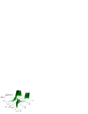
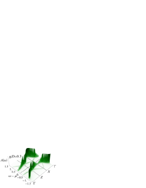
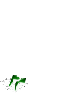
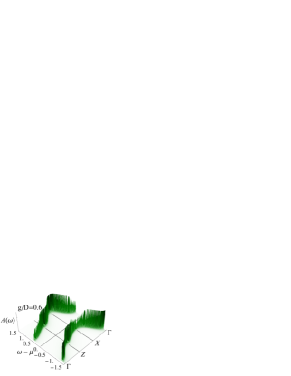
Figure 5: (Color online) Dispersion of the Bogoliubov branches $E_{i}$ and the related spectral weight at zero temperature for the $c$-type excitation as a function of the exchange coupling. From top to the bottom the exchange assumes the following values: $g/D=0.1,0.3,0.4,0.6$, respectively. The points of the two dimensional Brillouin zone are: $\Gamma=[0,0],Z=[\pi,0],X=[\pi,\pi]$.

In our investigation of the various phases of the BFM, let us start with by examining the evolution of the charge gap, as extracted from the density of states, $N_{c}(\omega)=\int d\epsilon N(\epsilon)A^{c}_{k}(\omega)$, with $A^{c}_{k}(\omega)=(-1/\pi)Im[G^{c}_{k}(\omega)]$ and $N(\epsilon)$ the bare density of states. Both in the SC- and the I-phase the $b$-bond bosons are condensed. Thus, the charge gap ($\Delta_{c}$) represents an estimate of the energy required to break a $b$-bond boson and create a pair of $h$- and $s$-bond fermions in case those bond fermions simply hybridize or pair up. As one can see from Fig.4, $\Delta_{c}$ has a non-monotonous behavior as the exchange coupling $g$ is varied from weak to strong coupling. For $g/D$ smaller than about $0.15$, the energy to excite a single $c$-type fermion grows slightly as a consequence of the concomitant effect of the constraint, the hybridization between the $s$- and $h$-bond fermions as well as the increasing pairing between them. Beyond $g/D\simeq 0.15$, the bond-hole boson amplitude diminishes, which drives the charge gap to a lower bound. Upon further increasing $g/D$, the systems transits from a superconducting to an insulating phase. The non-monotonic behavior occurring in the superconducting regime is related to the competition between the two possible channels for breaking a $b$-bond boson (see Fig.1b). Moving into the insulating side of the phase diagram, we notice that the charge gap increases almost linearly with $g$. This indicates that now, for breaking one $b$-bond boson in order to create a pair of $s$, $h$-bond fermions, one has to overcome the strength of the local exchange. In this limit, it is the constraint that determines the local scale of exchange energy in the excitation spectrum.

Up to now we have concentrated our attention on the amplitude of the $b$-bond bosons and their, related to it, charge gap and its evolution from the SC to the I phase. We next shall investigate how the dispersion and the related spectral weight associated with the $c$-type excitations of the Bogoliubov branches get modified by tuning the exchange coupling. In Fig. 5 we report the behavior of the spectral function for the original fermions as a function of their momentum, when moving along the major symmetry lines of the two-dimensional Brillouin zone.

We observe that the structure of the excitation spectra is qualitative different in the superconducting phase and the insulating one. We obtain four branches in the SC region and only two in the insulating one. Concerning the dispersion and the position where the charge gap opens, there are distinct differences in the two parts of the phase diagram. Starting from the weak coupling regime, one notices that the gap opens up at the $Z$ point of the Brillouin zone. This is due to a crossing at this point of the fermion-like and fermion-hole-like tight-binding spectrum, for the particle-hole symmetric half filled band case, studied here. Looking at the evolution of the spectral function, the excitations with the dominant weight follow a dispersion that is reminiscent of a free tight binding spectrum, except close to the $Z$ point, where the gap opens. Furthermore, in this region of coupling, two almost dispersionless branches with small spectral weights are present. They arise from the hybridization between the $s$- and $h$-bond fermions. Their small spectral weight is a consequence of a counter-active action between the $b$-bond and $d,f$-bond bosons in renormalizing the hybridization between the bond fermions. Increasing the exchange coupling induces a modification in the spectral weight distribution and in the width of the dispersion. The dominant Bogoliubov branches get more dispersive upon approaching the quantum phase transition due to an increase in the $b$-bond boson amplitude $\bar{b}$. Their spectral weight however diminishes down to zero due to the reduction of the bond-hole and double paired boson amplitudes $\bar{d}$ and $\bar{f}$ as we approach the quantum critical point. This change is accompanied by a partial redistribution of the spectral weight in the lower and upper Bogoliubov branches. Crossing the critical exchange coupling, the bands below (above) the chemical potential develop a unique structure and one no longer discerns any trace of the four Bogoliubov branches which were caused by the pairing and the hybridization between the bond-fermions. In this region, only the process of mixing the $s$- and $h$-bond fermions is active. Now, a $b$-bond boson can only break into a $s$- and $h$-bond fermion but the energy cost for that grows proportionally to the exchange coupling and is controlled by the constraint. The emerging bond-fermions have propagating features and hybridize with each other which results in a dispersion that is renormalized by the $b$-bond boson amplitude $\bar{b}$.

VI Conclusions

In the present study we have illustrated the evolution of pairing correlations in a two-component system where local bond pairing is induced in an ensemble of itinerant fermions. We have shown that there are two possible bond pair configurations which can materialize. Depending on whether we have a finite or a zero amplitude of the bond-hole (respectively double-paired-bond) bosons, we obtain a superconducting or an insulating phase. The bond fermions which emerge in such system control the occurrence of the one or the other bond pair liquid. Those bond fermions are both: (i) single fermions on a bond and (ii) fermions attached locally to a boson on that same bond. The dynamics of these bond fermions and the interplay between the related pairing and the hybridization process crucially determines the competition between the superconducting and the insulating paired liquid states.

To extract the main features of this scenario, we have used a bond operator formalism, which has been widely applied in the literature for the spin analogue quantum problems. In the present problem, it has turned out to be particularly useful because of the intrinsic nature of the dimer formation of resonant pairs. Moreover, though the bond operator method, within the present mean field approach, is best suited for the strong coupling limit, it can indeed describe the quantum phase transition because, as we have shown, it occurs in a regime of coupling where $g/t\sim 2$. This, a posteriori, justifies the use of an approximation that is based on a local saddle point ansatz for the bond bosons. Still, as we have discussed in the Introduction, it is already within the local structure of the bond configurations that one recovers the objects to distinguish between the superonducting and the insulating state. Among the non-bonding configurations, there is the bond-hole state, which turns out to be the relevant bond boson, because the formation of the superconducting state is attributed to the simultaneous presence of a phase coherent amplitude for the bonding bosons as well as for the bond holes. This is a key element that allows to follow the evolution from the insulating (condensation of the pure bonding bosons) to the superconducting state (pairing of the $s$ and $h$ fermions, due to the phase coherence of the bonding bosons and the bond holes).

We have obtained the phase diagram as a function of the boson-fermion exchange coupling and by varying the temperature. We have shown how, with increasing the exchange coupling, the continuous reduction of the amplitude of the bond-hole condensate drives the quantum phase transition between the superconducting and the insulating state. This behavior is dictated by the interplay between the dynamics of the bond fermions and the constraint controlling the occupation of the various bond operators. In this first attempt to capture the salient aspects of that scenario, on the basis of a mean field approach in the bond operator formulation of it, we have focused our attention on the excitation spectra and the nature of the charge gap. In the superconducting region the single particle gap exhibits a non-monotonic evolution as the exchange coupling is increased and the quantum phase transition is approached. This is a sign of the double nature of the dynamical variables at play and which contains features of pairing as well as of hybridization of those bond fermions. A completely different behavior characterizes the insulating regime where it is the local exchange which sets the scale of energy. Coming from the insulating side, entering the superconducting phase one is led to the picture where the insulating charge gap continues to exist in the superconducting phase as one of the components of the charge gap, and whose amplitude diminishes as $g$ goes to zero. This could signify a breakdown in cascade of the order in such systems, as $g$ is increased. First destroying the superconducting phase but without the amplitude of the pairs up to the quantum critical point and then destroying gradually the pair amplitude when $g$ is sufficiently large in the insulating state.

Concerning the excitation spectra, there are four Bogoliubov branches in the superconducting region and which continuously evolve into a two branch configuration in the insulating region. For a 2-dimensional system and the corresponding tight-binding spectrum for the original bare fermions, the pairing gap opens up at the $Z$ point of the Brillouin zone. The interplay between the pairing and the hybridization between the bond fermions also controls the spectral weight redistribution between the various Bogoliubov branches as the exchange coupling is tuned through the quantum phase transition.

Further analysis on the issues which have been discussed here is presently in progress and deals with such questions as the effects expected for hole doping away from the half-filled band case and of the feedback on the bond fermions arising from the dynamics of the bond bosons. A major attempt in this direction will concern the case when the system is in the proximity of the breakdown of the coherent superconducting state where possibly a metallic phase of bosonic fermion pairs could exist. For that purpose the present bond-mean-field analysis will be improved by taking into account the phase fluctuations of the bosonic mean field coherent states desribed here.

References

- (1) P. Phillips and D. Dalidovich, Science 302, 243 (2003) and references therein.
- (2) P.A. Lee, N. Nagaosa, and X-G Wen, Rev. Mod. Phys. 78, 17 (2006) and references therein.
- (3) H. M. Jaeger, D. B. Haviland, B. G. Orr, and A. M. Goldman, Phys. Rev. B 40, 182 (1989).
- (4) E. Ephron, A. Yazdani, A. Kapitulnik, and M. Beaseley, Phys. Rev. Lett., 76, 1529 (1996).
- (5) N. Mason and A. Kapitulnik, Phys. Rev. B 64, 60504 (2001).
- (6) S. Jochim, M. Bartenstein, A. Altmeyer, G. Hendl, S. Riedl, C. Chin, J. Hecker Denschlag, and R. Grimm, Science 302, 2101 (2003) and references therein.
- (7) J. Ranninger, J.-M. Robin and M. Eschrig, Phys. Rev. Lett. 74, 4027 (1995);J. Ranninger and S. Robaszkiewicz, Physica B 153B, 468 (1985).
- (8) J. Ranninger and A. Romano, Europhys. Letts. 75, 461 (2006).
- (9) S. R. White and D. J. Scalapino, Phys. Rev. B 55, 6504 (2002).
- (10) P. W. Anderson, Science 235, 1196 (1987).
- (11) E. Altman and A. Auerbach Phys. Rev. B 65, 104508 (1997).
- (12) H. Feshbach, Ann. Phys. (N.Y.) 55, 357 (1958).
- (13) E. Timmermans, P. Tommasini, M Hussein and A. Kerman, Phys. Rep. 315, 199 (1999).
- (14) S. Sachdev and R.N. Bhatt, Phys. Rev. B 41, 9323 (1990).
- (15) A.V. Chubukov and Th. Jolicoeur, Phys. Rev. B 44, 12050 (1991).
- (16) S. Gopalan, T.M. Rice, and M. Sigrist, Phys. Rev. B 49, 8901 (1994).
- (17) K. Park and S. Sachdev Phys. Rev. B 64, 184510 (2001).
- (18) E. Demler and S. Das Sarma, Phys. Rev. Lett. 82, 3895 (1999).
- (19) C. Jurecka and W. Brenig, Phys. Rev. B 64, 092406 (2001).
- (20) M. Cuoco and J. Ranninger, Phys. Rev. B 70, 104509 (2004) .
- (21) J. Ranninger and J.-M. Robin, Solid State Commun. 98, 559 (1996).