Comment on “Spurious fixed points in frustrated magnets,” cond-mat/0609285

Abstract

We critically discuss the arguments reported in cond-mat/0609285 by B. Delamotte, Yu. Holovatch, D. Ivaneyko, D. Mouhanna, and M. Tissier. We show that their conclusions are not theoretically founded. They are contradicted by theoretical arguments and numerical results. On the contrary, perturbative field theory provides a robust evidence for the existence of chiral fixed points in $O(2)\otimes O(N)$ systems with $N\geq 2$. The three-dimensional perturbative results are consistent with theory and with all available experimental and Monte Carlo results. They provide a consistent scenario for the critical behavior of chiral systems.

In Ref. [1] the authors provide what they think is evidence against the presence of a stable fixed point (FP) in $O(2)\otimes O(N)$ models for $N=2,3$, contradicting the results of Refs. [2, 3] obtained by the analysis of high-order perturbative series (see, e.g., Ref. [4] for a discussion of the method). In this Comment we show that their arguments are either theoretically incorrect or contradictory.

Fixed points in four dimensions. The main argument against the presence of a stable FP for $N=2,3$ is based on the claim that a physical FP of a given Hamiltonian must survive up to $d=4$ (i.e. up to $\epsilon\equiv 4-d=0$) and become the Gaussian FP in this limit. There is no theoretical justification for this requirement: the authors of Ref. [1] do not provide any motivation, they simply state it must be so. Note that this condition is very restrictive and contradicts several well-accepted theoretical results. For $\epsilon\ll 1$, the chiral FP $C_{+}$ exists only for $N\gtrsim 21.8$. Thus, according to this criterion, all FPs with $N\lesssim 21.8$ should be considered as spurious! This is in contradiction with the results obtained in all approaches: indeed, for $N>6$ all methods agree and predict a stable FP. We must observe that the perturbative results of Ref. [3] find no difference between the FPs with $N\gtrsim 6$ (on whose existence there is no discussion) and those with $N\lesssim 6$: the FP position varies smoothly with $N$ and $d$. Thus, the difference between the perturbative results and those obtained by using the functional renormalization group (FRG) [5, 6, 7] is only quantitative: the two methods disagree on the behavior of the function $N_{c}(\epsilon)$ or of its inverse $\epsilon_{c}(N)$ for $\epsilon\approx 1$ (see the discussion in Sec. II.D of Ref. [3]). But there are no conceptual differences as the authors of Ref. [1] apparently imply.

The behavior observed here is analogous to that found in the Ginzburg-Landau model of superconductors. Close to 4 dimensions a FP is found only for $N\gtrsim 365.9$ ($N$ is the number of components of the scalar field) [8]. The criterion proposed in Ref. [1] would thus predict a first-order transition for the physical case $N=1$, contradicting experiments [9], and also general duality arguments [10], FRG calculations [11], and Monte Carlo simulations [12]. Fixed-dimension calculations are instead consistent with the existence of a stable FP [13, 14].

As we already said, we do not think that the behavior in four dimensions is of any relevance for the three-dimensional theory. There is instead another condition that is crucial: the three-dimensional FP must be connected by the three-dimensional renormalization-group flow to the Gaussian FP [4, 15]. If this is the case, at least for the massive zero-momentum (MZM) scheme, one can give a rigorous nonperturbative definition of the renormalization-group flow and of all quantities that are computed in perturbation theory. One may consider weakly coupled models or models with medium-range interactions, as discussed in Sec. III.B of Ref. [3]. These models are defined on the lattice and as such are well defined nonperturbatively. In a well-defined limit (see Sec. III.B of Ref. [3]) long-range quantities (correlation length, susceptibilities, etc.) have the same perturbative expansion as the corresponding quantities in the continuum theory in the MZM scheme. The existence of a stable FP is equivalent to the existence of a second-order transition for small but finite values of the bare quartic coupling constants (weakly coupled models) or for large but finite values of the interaction range (medium-range systems). Note that everything is defined nonperturbatively and rigorously in three dimensions and there is no need of invoking the existence of a four-dimensional FP.

The chiral fixed points for $d\to 4$. In Ref. [1] it was claimed that for $N=2,3$ one can follow the FP $C_{+}$ up to $d=4$. This statement is incorrect and is based on an incorrect use of the conformal-mapping method. To explain this point let us review the results of the semiclassical analysis for the Borel singularities. For $u\geq 0$ and $v\leq 2u$ the perturbative series are Borel summable. Thus, under the assumption that all singularities lie on the negative real axis in the Borel plane, the conformal-mapping method transforms the original asymptotic series into a convergent one. If $2u\leq v\leq 4u$ the perturbative series are not Borel summable: there is a singularity on the positive real axis. However, in this range of values of $v$ the Borel singularity that is closest to the origin is still on the negative real axis. Thus, the conformal-mapping method still takes into account the large-order behavior. Though the resulting resummed series is only asymptotic, its coefficients should increase slower than those of the original one. For these values of $v$ one may expect to obtain reasonable results out of six- or five-loop perturbation theory, though not so precise as those that are obtained in $O(N)$ models. If $v\geq 4u$ the leading singularity is on the positive real axis and thus the conformal-mapping method cannot be used: the function $\omega(u;z)$ (defined in Eq. (2) of Ref. [1]) becomes imaginary for $u=-1/a$ if $a$ is negative. For this reason, as discussed in Ref. [3], one cannot follow the FPs that exist for $N=2$ and $3$ for $d\gtrsim 3.3$. Probably, Fig. 4 of Ref. [1] has been obtained by always using $a=u/2$, which means that for $v\geq 4u$ the resummation does not take into account the leading large-order behavior: the resummed perturbative series diverge exactly as the original ones. Unresummed perturbative series are not very predictive and the most accurate results (we use the word accurate in the sense of least difference between estimate and exact result, as usual in the context of asymptotic series) are obtained at very low orders. For instance, in the absence of a Borel resummation, the standard $\epsilon$ expansion for $O(N)$ models gives the most accurate results at two loops [16]: inclusion of higher-order terms worsens the estimates and indeed unresummed five-loop estimates have no relation with the correct asymptotic result. The same occurs in the MZM scheme. Thus, the results of Ref. [1] for the existence of FPs for $N=2,3$ in the intermediate region $3.3\leq d\leq 4$ cannot be trusted.

Numerical results. The authors of Ref. [1] claim that the existence of a stable FP contradicts presently available numerical results. Instead, there are no contradictions: All numerical and experimental results are consistent with the predictions of perturbative field theory. First, let us remind the reader that the existence of a stable FP does not imply that all systems with the given symmetry undergo a second-order phase transition. The transition is continuous only if the system is in the basin of attraction of the stable FP. For instance, in systems with a scalar order parameter one may observe a first-order transition or a second-order transition belonging to the Ising universality class; with an appropriate tuning of the parameters it is also possible to have a tricritical point. First-order transitions in scalar systems are perfectly compatible with the existence of the Ising universality class! Thus, the quoted results [17, 18, 19] are irrelevant for the discussion: the first-order nature of the transition in XY stacked antiferromagnets (not to be confused with the easy-plane antiferromagnets studied experimentally, see the discussion in Sec. V of Ref. [3]) is consistent both with the presence and with the absence of an $N=2$ chiral FP. On the other hand, the results of Ref. [3] and of Ref. [20]—they find continuous transitions for $N=2$ and $N=3$, respectively—are only consistent with the presence of a stable FP and thus do not support the scenario of Ref. [1]. Thus, at variance with the claim of Ref. [1], numerical results are not consistent with the scenario that all chiral systems with $N=2$ and $N=3$ undergo first-order transitions.

Experimental results. Ref. [1] states that experiments contradict the perturbative results. Again, we must stress that this is not the case. First, we must note that the results of Ref. [21] cited in Ref. [1] are perfectly consistent with perturbation theory. We discussed in detail easy-axis systems in Ref. [22] and showed two possible phase diagrams compatible with perturbation theory, see Fig. 3 of Ref. [22]. The results of Ref. [21] correspond exactly to phase diagram (b) reported in Fig. 3 of Ref. [22]. As for easy-plane systems, all experiments observe continuous transitions, and thus they are compatible with the perturbative results (but not with those of Refs. [5, 6, 7]). In any case, note that perturbation theory does not predict easy-plane systems (or any model) to have a continuous transition. It only predicts that, if the transition is continuous, it should belong to the chiral universality class. In Refs. [5, 6, 7] it was remarked that, even if experiments observe continuous transitions, the measured critical exponents in some cases do not satisfy rigorous inequalities, for instance $\beta\geq\nu/2$. In Ref. [3] we showed that this may be explained by corrections to scaling. Due to the “focus”-like nature of the FP [23] the approach to criticality may be quite complex. Effective exponents may even change nonmonotonically, at variance with what occurs in $N$-vector models (for the effective exponents in $O(N)$ models, see Refs. [24, 25]).

In conclusion, the statement of Ref. [1] on the experiments is biased and not justified by the experimental results.

The cubic model. The authors of Ref. [1] also discuss the cubic model defined in their Eq. (4). They assume the well-established scenario provided by the $\epsilon$ expansion: no FP is present in the domain $v<0$. Then, they analyze the perturbative series for the model in the minimal-subtraction scheme without $\epsilon$-expansion ($3d$-$\overline{\rm MS}$ scheme) and find some evidence for a FP with $v<0$. Since this FP is not predicted by the $\epsilon$ expansion they conclude that this FP is spurious. Hence—they conclude—perturbation theory cannot be trusted.

Again, the presentation is strongly biased. First, it is not clear to us which results support the claim that the physics of systems with cubic anisotropy is well established. Indeed, all references that are cited and that discuss the behavior for $v<0$ assume that the $\epsilon$ expansion is predictive in three dimensions. But, of course, one cannot take this for granted in this discussion, since the debate is exactly on the quantitative predictivity of the $\epsilon$ expansion. Beside the $\epsilon$-expansion investigations, there are only a few numerical works for the antiferromagnetic four-state Potts model on a cubic lattice [26, 27, 28], whose critical behavior should be described by the $N=3$ cubic model with $v<0$ [29]. Contrary to the claim of Ref. [1], all numerical results are consistent with a continuous transition: at present there is no evidence of first-order transitions. Thus, the behavior of this class of systems is not at all well established, but appears as rather controversial. Therefore, it is worthwhile to check whether a FP with $v<0$ exists or not, without any a priori preconception.

For this purpose we have repeated the analysis of the 5-loop perturbative series for the cubic model in the $3d$-$\overline{\rm MS}$ scheme discussed in Ref. [1] and we have also analyzed the 6-loop perturbative series of Ref. [30] in the MZM scheme. We focus on $v<0$ and $N=3$. For each $b$ and $\alpha$ (defined in Ref. [1] or, equivalently in Ref. [30]) we resum the $\beta$ functions, look for a common zero, and, if present, determine its stability. We vary $\alpha$ and $b$ in the intervals $-1\leq\alpha\leq 5$ and $2\leq b\leq 20$: in practice, we consider 133 different resummations. In the $3d$-$\overline{\rm MS}$ scheme a FP is found in 91/133 cases; it is stable in 54/133 cases. In the MZM scheme only 67 resummations find a FP; only in 61 cases is the FP stable. The evidence for a stable FP is not overwhelming: in both cases a stable FP is observed in less than 50% of the resummations. It is also interesting to look for the scatter of the estimates of the FP, see Fig. 1. The estimate of the FP position varies significantly ($u^{*}$ changes by a factor of 2 in the $3d$-$\overline{\rm MS}$ scheme and by 20% in the MZM scheme) and thus it is not clear how much one can trust the estimates. Thus, contrary to the claim of Ref. [1], the analysis of the perturbative series does not provide compelling evidence for the existence of a new FP in cubic models with $v<0$ and $N=3$. The evidence is even worse for larger values of $N$.

In Ref. [1] it was claimed that the cubic-model results show similar convergence properties as in the frustrated case. This statement, given without any quantitative comparison, is completely unjustified. For instance, in the MZM case, by using the same analysis reported above one finds a FP in 121 cases; the FP is always stable. While in the cubic case a stable FP is observed in less than 50% of the cases, in the chiral case a stable FP is observed in 92% of the cases—not a negligible difference! The difference between the two cases is even better understood if one compares the FP position, see Fig. 2. Differences are so evident, that no additional comment is needed!

Reconciling the different approaches. To conclude this Comment we would like to go back to the original motivation of Ref. [1] (see also Ref. [7]), the discrepancy between the perturbative results and those obtained in Refs. [5, 6, 7], where the FRG approach was used at order $\partial^{2}$ (first order of the derivative expansion). In Refs. [6, 7] it was noted that, though no FP point was observed, there was a region in which the $\beta$ functions were small, giving rise to a very peculiar slowing down of the renormalization-group flow. Correspondingly, the integration of the flow equations led generically to good power laws (pseudoscaling) for the interesting thermodynamical observables. The presence of quasi-scaling in the FRG calculations suggests a way of reconciling the two approaches: it may be possible that by improving the approximations in the FRG calculation, this approximate scaling may turn into a real one with the presence of a true fixed point. In other words the differences may simply be due to the crudeness of the approximations used in Refs. [5, 6, 7]. This interpretation is supported by the fact that the effective exponents obtained by using the FRG are very close to those obtained by using perturbative field theory. For instance, for $N=3$ Ref. [7] predicts (see Table XI)

$\displaystyle\nu\approx 0.54,\qquad\qquad\beta\approx 0.29$

to be compared with the MZM results

$\displaystyle\nu=0.55(3),\qquad\qquad\beta=0.30(2).$

It is worth mentioning that a similar phenomenon is observed in the two-dimensional XY model [31]. This model shows a line of FPs in the low-temperature phase below the Kosterlitz-Thouless transition. FRG calculations at order $\partial^{2}$ do not observe this FP line: the $\beta$-function never vanishes in the low-temperature phase. Nonetheless, a clear signature of the presence of the line of FPs is present: the $\beta$ functions are very small and quasi-scaling is observed with good accuracy in the whole low-temperature phase. The same phenomenon may occur in chiral models.

Conclusions. The perturbative field-theory results of Refs. [2, 3] are consistent with theory and with all available experimental and Monte Carlo calculations, providing a consistent scenario for the critical behavior of chiral systems. They only disagree with FRG calculations at order $\partial^{2}$. Note, however, that, even if they do not find a stable FP, nonetheless they observe quasiscaling both for $N=2$ and $N=3$. One may conjecture that this quasiscaling turns into real scaling (with the existence of a stable FP) by improving the approximations. This would reconcile the two approaches.

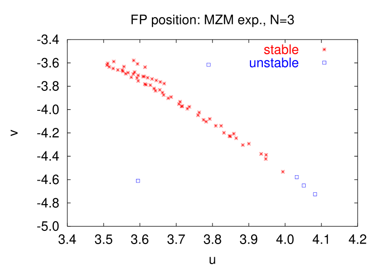
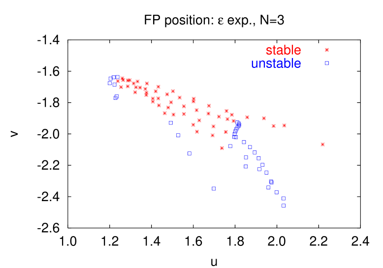
FIG. 1.: Perturbative results for the cubic model with $N=3$ and $v<0$: Fixed-point position. Above we report the MZM results, below the $3d$-${\overline{\rm MS}}$ results.

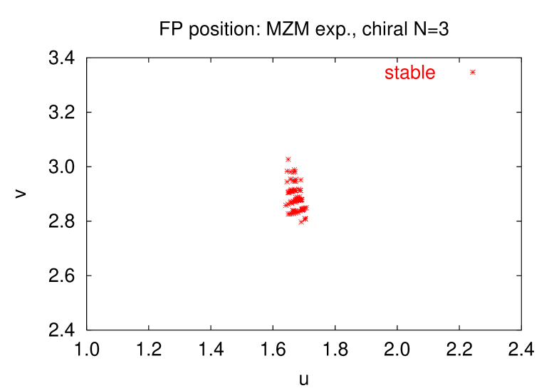
FIG. 2.: Perturbative results for the chiral model with $N=3$ and $v>0$: Fixed-point position in the MZM scheme. Note that the horizontal scale is analogous to that used to show the $3d$-${\overline{\rm MS}}$ results for the cubic model. All FPs are stable.

REFERENCES

- [1] B. Delamotte, Yu. Holovatch, D. Ivaneyko, D. Mouhanna, and M. Tissier, cond-mat/0609285.
- [2] A. Pelissetto, P. Rossi, and E. Vicari, Phys. Rev. B 63, 140414(R) (2001).
- [3] P. Calabrese, P. Parruccini, A. Pelissetto, and E. Vicari, Phys. Rev. B 70, 174439 (2004).
- [4] J. Zinn-Justin, Quantum Field Theory and Critical Phenomena, fourth edition (Clarendon Press, Oxford, 2001).
- [5] M. Tissier, B. Delamotte, and D. Mouhanna, Phys. Rev. Lett. 84, 5208 (2000).
- [6] M. Tissier, B. Delamotte, and D. Mouhanna, Phys. Rev. B 67, 134422 (2003).
- [7] B. Delamotte, D. Mouhanna, and M. Tissier, Phys. Rev. B 69, 134413 (2004).
- [8] B.I. Halperin, T.C. Lubensky, and S.K. Ma, Phys. Rev. Lett. 32, 292 (1974).
- [9] C.W. Garland and G. Nounesis, Phys. Rev. E 49, 2964 (1994).
- [10] H. Kleinert, Gauge Fields in Condensed Matter (World Scientific, Singapore 1989).
- [11] B. Bergerhoff, F. Freire, D.F. Litim, S. Lola, and C. Wetterich, Phys. Rev. B 53, 5734 (1996); B. Bergerhoff, D.F. Litim, S. Lola, and C. Wetterich, Int. J. Mod. Phys. A 11, 4273 (1996).
- [12] S. Mo, J. Hove, and A. Sudbø, Phys. Rev. B 65, 104501 (2002).
- [13] I. F. Herbut and Z. Tešanović, Phys. Rev. Lett. 76, 4588 (1996).
- [14] R. Folk and Yu. Holovatch, J. Phys. A 29, 3409 (1996); in Correlations, Coherence, and Order, Proceedings of the 1st Pamporovo Winter Workshop on Cooperative Phenomena in Condensed Matter, March 1998, Pamporovo, Bulgaria, edited by D. V. Shopova and D. I. Uzunov (Plenum, London–New York, 1999), cond-mat/9807421.
- [15] C. Itzykson and J.M. Drouffe, Statistical Field Theory (Cambridge Univ. Press, Cambridge, UK, 1989).
- [16] E. Brézin, J.C. Le Guillou, J. Zinn-Justin, and B.G. Nickel, Phys. Lett. 44A, 227 (1973).
- [17] M. Itakura, J. Phys. Soc. Jpn. 72, 74 (2003).
- [18] A. Peles, B. W. Southern, B. Delamotte, D. Mouhanna, and M. Tissier, Phys. Rev. B 69, 220408 (2004).
- [19] S. Bekhechi, B. Southern, A. Peles, and D. Mouhanna, Phys. Rev. E 74, 016109 (2006).
- [20] A. Peles and B.W. Southern, Phys. Rev. B 67, 184407 (2003).
- [21] G. Quirion, X. Han, M.L. Plumer, and M. Poirier, Phys. Rev. Lett. 97, 077202 (2006).
- [22] P. Calabrese, A. Pelissetto, and E. Vicari, Nucl. Phys. B 709, 550 (2005).
- [23] P. Calabrese, P. Parruccini, and A.I. Sokolov, Phys. Rev. B 66, 180403(R) (2002); Phys. Rev. B 68, 094415 (2003).
- [24] C. Bagnuls and C. Bervillier, Phys. Rev. B 32, 7209 (1985); Phys. Rev. E 65, 066132 (2002).
- [25] A. Pelissetto, P. Rossi, and E. Vicari, Nucl. Phys. B 554, 552 (1999).
- [26] Y. Ueno, G. Sun, and I. Ono, J. Phys. Soc. Jpn. 58, 1162 (1989).
- [27] M. Itakura, Phys. Rev. B 60, 6558 (1999).
- [28] C. Yamaguchi and Y. Okabe, J. Phys. A 34, 8781 (2001).
- [29] J.R. Banavar, G. S. Grest, and D. Jasnow, Phys. Rev. Lett. 45, 1424 (1980); Phys. Rev. B 25, 4639 (1982).
- [30] J.M. Carmona, A. Pelissetto, and E. Vicari, Phys. Rev. B 61, 15136 (2000).
- [31] G. von Gersdorff and C. Wetterich, Phys. Rev. B 64, 054513 (2001).