Angular velocity distribution of a granular planar rotator in a thermalized bath

Abstract

The kinetics of a granular planar rotator with a fixed center undergoing inelastic collisions with bath particles is analyzed both numerically and analytically by means of the Boltzmann equation. The angular velocity distribution evolves from quasi-gaussian in the Brownian limit to an algebraic decay in the limit of an infinitely light particle. In addition, we compare this model with a planar rotator with a free center. We propose experimental tests that might confirm the predicted behaviors.

I Introduction

When macroscopic particles undergo inelastic collisions the total kinetic energy decreases with time. If an external source of energy, such as a vibrating bottom wall, is present, the system may reach a stationary state. Despite similarities with equilibrium systems, however, equilibrium statistical mechanical concepts cannot be appliedGoldhirsch (2003); Brilliantov and Pöschel (2004); Zippelius (2006). For instance, there is no equipartition between different species in polydisperse systemsWildman and Parker (2002); Feitosa and Menon (2002); Martin and Piasecki (1999); Huthmann et al. (1999); Barrat and Trizac (2002), and velocity distributions are, in general, non-gaussianBrey et al. (1999); Rouyer and Menon (2000); Atwell and Olafsen (2005).

In dilute systems, most collisions only involve two particles, and consequently, a theoretical description of the dynamics has been proposed starting from the Boltzmann or Enskog equationPöschel and Brilliantov (2003); Brilliantov and Pöschel (2004).

The inelastic hard sphere model is a paradigm for granular gases in the same way that the elastic hard sphere model is for equilibrium fluidsBrilliantov and Pöschel (2004). While both account for the exclusion effect, energy is lost at each collision in the former. For dissipative systems, recent studies have shown the relevance of the granular temperature, even if the absence of equipartition yields a number of temperatures increasing with the polydispersity or the number of degrees of freedom of each particle.

Few studies have addressed the effect of particle shape on the properties of granular gases. In three dimensions, Aspelmeier et alHuthmann et al. (1999) showed that the rotational and translational temperatures are different in the free cooling state of inelastic hard needles. Anisotropic tracers (needle and spherocylinder) in a thermalized bath also display non-equipartition between different degrees of freedomViot and Talbot (2004); Gomart et al. (2005). The purpose of this paper is to build a simple model which captures the specific features due to the shape of the particle and the presence of an irreversible microscopic dynamics.

We present here an investigation of the stationary kinetics of a planar rotator with a fixed center that undergoes inelastic collisions with the bath particles. With these assumptions, the kinetics is described by a linear Boltzmann equation. We show that, when the tracer is much heavier than the bath particle, the angular velocity distribution function is quasi-gaussian (the Brownian limit) whereas it exhibits an algebraic decay in the opposite limit of an infinitely light granular particlePiasecki and Viot (2006). For all intermediate cases, there is no simple scaling regime and deviations from gaussian behavior are captured by analyzing the fourth moment of the distribution function.

The paper is organized as follows: the model, its mechanical properties and the Boltzmann equation are presented in section II. The asymptotic solution of the Boltzmann equation in the Brownian limit is presented in section III. In section IV, analytical results are derived for a zero-mass limit and for different coefficients of restitution and intermediate cases are considered in section V. In section VI we compare the fixed rotator with one whose center is free, both within the gaussian approximation. Finally, the conclusion discusses possible experimental tests of our theoretical results.

II The planar rotator

II.1 Definition and mechanical properties

The model consists of a two-dimensional, infinitely thin needle of mass $M$, length $L$ and moment of inertia $I=ML^{2}/12$ immersed in a bath of point particles, each of mass $m$. The needle has a fixed center of mass, but can rotate freely around its center. It undergoes instantaneous and inelastic collisions with the surrounding bath particles. The motion of the planar rotator can be described with the angle between a unit vector ${\bf u}$ collinear to the axis of the needle and the x-axis.

The rate of change of the orientation $\dot{{\bf u}}=\omega{\bf u}_{\perp}$ is equal to the angular velocity $\omega\in]-\infty,+\infty[$ times a unit vector ${\bf u}_{\perp}$ perpendicular to ${\bf u}$.

The angular velocity of the rotator changes at each binary collision with a bath particle. The position of the point of impact along the needle axis is denoted by $\lambda{\bf u}$. Obviously, a condition for collision is $|\lambda|<L/2$ (see Fig.1). The relative velocity ${\bf V}$ at the point of impact equals

$${\bf V}={\bf v}-\lambda\dot{\bf u}={\bf v}-\lambda\omega{\bf u}_{\perp}$$ (1)

where ${\bf v}$ denotes the velocity of the bath particle.

Due to the dissipative nature of the collision, the relative velocity changes according to the collision law

$$V^{*}_{\perp} =-\alpha V_{\perp}$$ (2)

$$V^{*}_{||} =V_{||}$$ (3)

where $0\leq\alpha\leq 1$ is the normal restitution coefficient and where the indices $\perp$ and $||$ indicate the perpendicular and parallel components of any vector relative to the needle axis, respectively. When $\alpha=1$, one recovers an elastic collision rule. For the sake of simplicity, the tangential component of the velocity is unchanged during the collision.

Since each collision conserves the total angular momentum we have that

$$I\omega^{*}+\lambda mv^{*}_{\perp}=I\omega+\lambda mv_{\perp},$$ (4)

where post-collisional quantities are denote with a star.

By combining Eqs. (1)-(3), the post-collisional bath particle velocity is given by

$$v^{*}_{\perp}=v_{\perp}-\frac{I(1+\alpha)V_{\perp}}{I+m\lambda^{2}}.$$ (5)

whereas the corresponding post-collisional angular velocity is

$$\omega^{*}=\omega+\frac{(1+\alpha)V_{\perp}m\lambda}{I+m\lambda^{2}}.$$ (6)

The inverse transformation (giving the pre-collisional quantities denoted by a double star) is obtained by substituting $\alpha$ by $\alpha^{-1}$ and the starred quantities by double-starred quantities.

II.2 Homogeneous Boltzmann equation

At low density, one assumes that the needle influences weakly the local density of the bath and, consequently, that the system remains homogeneous. After a transient time (not considered here) the kinetics of the needle becomes stationary and can be described by the stationary Boltzmann equation. This expresses the invariance of the rotator angular velocity distribution function, $F(\omega)$, resulting from a balance between collisional gain and loss terms:

$$\int_{-L/2}^{L/2}\!\!d\lambda \int\!d{\bf v}|v_{\perp}-\lambda\omega|\left(\frac{F(\omega^{**})\Phi_{B}({\bf v}^{**})}{\alpha^{2}}-F(\omega)\Phi_{B}({\bf v})\right)$$

$$=0,s$$ (7)

where the pre-collisionnal velocities ${\bf v}^{**}$ and $\omega^{**}$ are given by the right hand sides of equations (5) and (6), respectively, with $\alpha$ replaced by $\alpha^{-1}$. $\Phi_{B}({\bf v})$ is the time independent bath velocity distribution.

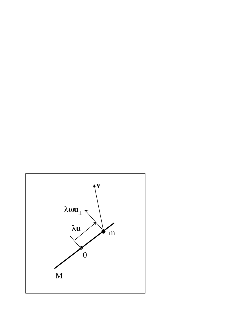
Figure 1: Illustration of a collision between the planar rotator and a bath particle: ${\bf u}$ and ${\bf u}^{\perp}$ are unit vectors parallel and perpendicular to the axis of the rotator. The element of the needle at $\lambda{\bf u}$ moves with linear velocity ${\lambda\omega\bf u}^{\perp}$.

The integration over the parallel velocity component $v_{||}$ in Eq.(II.2) can be readily carried out since $F$ does not depend of this variable. By changing of the integration variable we can rewrite Eq.(II.2) as

$$\int_{-L/2}^{L/2}d\lambda\int dv_{\perp}|v_{\perp}|\left[F\left(w+v_{\perp}\frac{(1+\alpha)m\lambda}{I+m\lambda^{2}}\right)\right.$$

$$\left.\phi_{B}\left(\lambda\omega+v_{\perp}\frac{(\alpha m\lambda^{2}-I)}{I+m\lambda^{2}}\right)-F(\omega)\phi_{B}(v_{\perp}+\lambda\omega)\right]=0,$$ (8)

with $\phi_{B}(v)=\int dv_{||}\Phi_{B}(|{\bf v}|)$.

III Brownian limit

An exact solution of Eq.(II.2) cannot be obtained in general. When the mass of the planar rotator is much larger than the mass of the bath particle, however, one expects that the deviation from Maxwellian behavior is weak. It turns out (see Appendix A) that exploring the regime corresponding to Brownian motion is equivalent to the analysis of the small $\lambda$ expansion of the collision term (8). We thus perform perform a perturbative expansion of the integrand of Eq.(II.2) in terms of $\lambda$. We denote

$$G(v_{\perp},\omega,\lambda)=\left[F\left(w+v_{\perp}\frac{(1+\alpha)m\lambda}{I+m\lambda^{2}}\right)\right.$$

$$\left.\phi_{B}\left(\lambda\omega+v_{\perp}\frac{(\alpha m\lambda^{2}-I)}{I+m\lambda^{2}}\right)-F(\omega)\phi_{B}(v_{\perp}+\lambda\omega)\right]$$ (9)

with the property that $G(v_{\perp},\omega,0)=0$. To go further, we assume in the rest of this section that the bath distribution, $\phi_{B}(v)$, is a Maxwellian:

$$\phi_{B}(v)=\phi_{M}(v)=\sqrt{\frac{m}{2\pi T}}\exp(-mv^{2}/2T)$$ (10)

The first derivative of $G(v_{\perp},\omega,\lambda)$ with respect to $\lambda$ at $\lambda=0$ gives the differential equation

$$(1+\alpha)\frac{dF(\omega)}{d\omega}+2F(\omega)\frac{\omega I}{T}=0$$ (11)

whose solution is

$$F(\omega)\propto\exp\left(-\frac{I\omega^{2}}{(1+\alpha)T}\right)$$ (12)

By taking the second derivative, one obtains the differential equation

$$(1+\alpha)\frac{d^{2}F(\omega)}{d\omega^{2}}+\frac{2I}{T}\omega\frac{dF(\omega)}{d\omega}+\frac{2I}{T}F(\omega)=0$$ (13)

whose solution is also given by Eq.(12).

The third-order expansion gives a polynomial in $v_{\perp}$

$$\frac{m^{3}v_{\perp}^{3}}{I^{3}}H_{3}\left(F(\omega)\right)-\frac{3m^{2}v_{\perp}}{I^{2}}H_{1}\left(F(\omega)\right)=0$$ (14)

where

$$H_{3}\left(F(\omega)\right) =(1+\alpha)^{3}\frac{d^{3}F(\omega)}{d\omega^{3}}+3(1+\alpha)^{2}\frac{I\omega}{T}\frac{d^{2}F(\omega)}{d\omega^{2}}+$$

$$+3\frac{I}{T}\left((1+\alpha)\frac{I\omega^{2}}{T}+2\right)\frac{dF(\omega)}{d\omega}+$$

$$+\frac{2I^{2}\omega}{T^{2}}\left(3(1+\alpha)+\frac{I\omega^{2}}{T}\right)F(\omega)$$ (15)

and

$$H_{1}\left(F(\omega)\right) =(1+\alpha)(2+\frac{I\omega^{2}}{T})\frac{dF(\omega)}{d\omega}+$$

$$+\frac{I\omega}{T}\left((1+\alpha)+2\frac{I\omega^{2}}{T}\right)F(\omega)$$ (16)

The solution of $H_{3}=0$ is given by Eq.(12) again, but the solution of $H_{1}=0$ is

$$F(\omega)\sim\left(2+\frac{I\omega^{2}}{T}\right)^{\frac{1-\alpha}{1+\alpha}}\exp\left(\frac{-I\omega^{2}}{(1+\alpha)T}\right)$$ (17)

If Eq.(17) if different from Eq.(12), it is interesting to note that this solution is the same Maxwellian times a slow decreasing function (If $\alpha=1$, Eq.(17) is identical to Eq.(12)). The fourth derivative of $G(v_{\perp},\omega,\lambda)$ has been calculated with the software Maple, and it occurs that the differential equation associated with the $v_{\perp}^{3}$ term has a Maxwellian solution but the solution of the differential equations associated with the $v_{\perp}$-term is given by the Maxwellian solution multiplied by a slow varying function. Therefore, we conjecture that the complete solution is given by Eq.(12) times a sub-dominant term.

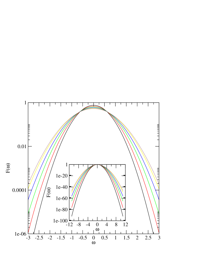
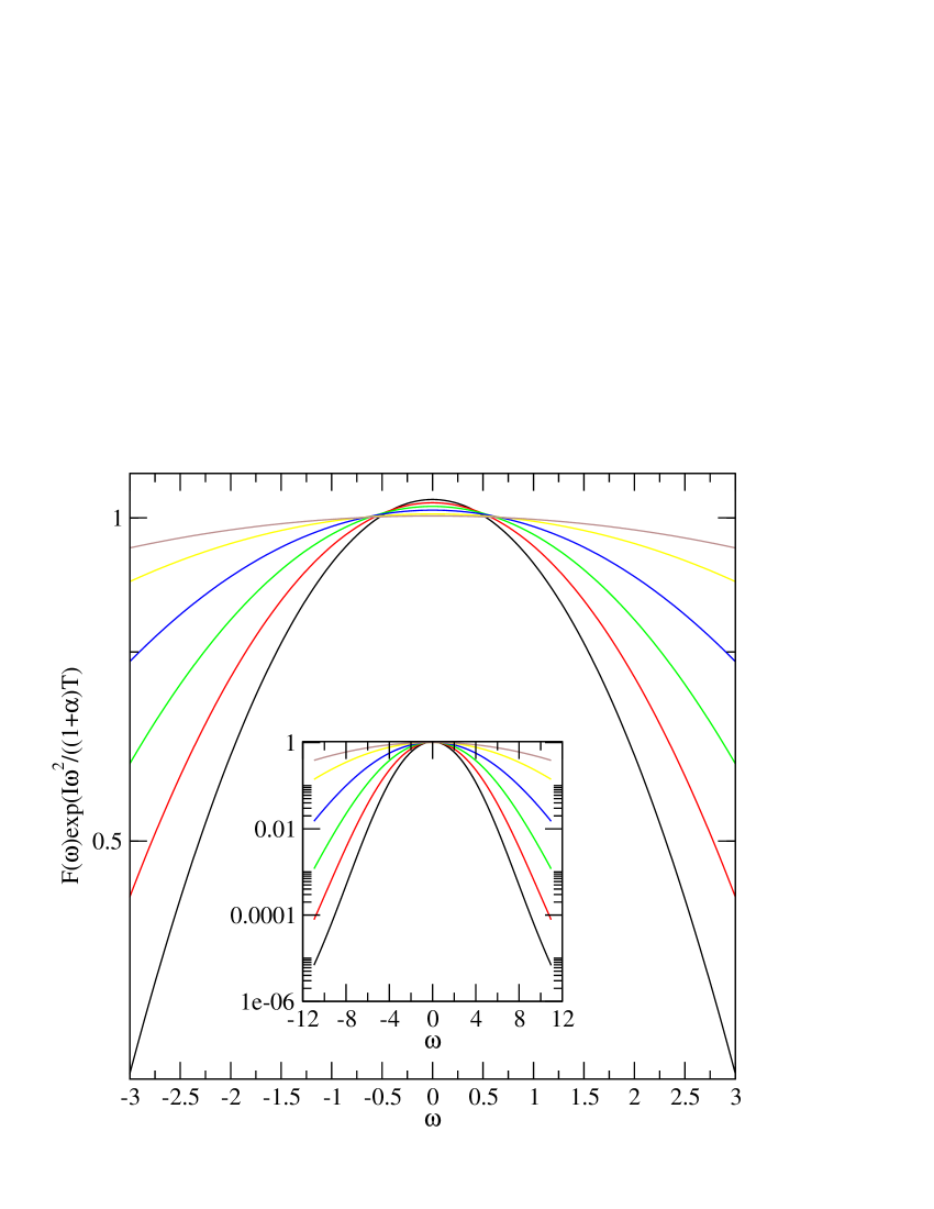
Figure 2: (a) Log-linear plot $F(\omega)$ for $M/m=10$ and with different values of the coefficient of restitution $\alpha=0,0.2,0.4,0.6,0.8,0.9$ (from top to bottom, center).(b) Log-linear plot $F(\omega)\exp(I\omega^{2}/((1+\alpha)T))$ for $M/m=10$. The insets display the same curves on a larger range of angular velocities.

In order to check this assumption, we have solved numerically the Boltzmann equation. Since Eq.(II.2) is linear and the distribution $F(\omega)$ is a one-variable function, we have used an iterative method that is very efficient and provides a much more accurate solutionBiben et al. (2002) than a DSMC methodMontanero and Santos (2000).

By using Eq.(II.2), the numerical resolution is obtained by iterating the following equation

$$F^{(n+1)}(\omega)= C(\omega)\int d\lambda\int dv|v|F^{(n)}\left(w+v\frac{(1+\alpha)m\lambda}{I+m\lambda^{2}}\right)$$

$$\phi_{M}\left(\lambda\omega+v\frac{(\alpha m\lambda^{2}-I)}{I+m\lambda^{2}}\right)$$ (18)

where

$$C(\omega)=\left(\int d\lambda\int dv|v-\lambda\omega|\phi_{M}(v)\right)^{-1}$$ (19)

$C(\omega)$ is an explicit function when the bath particle distribution $\phi_{M}(v)$ is a Maxwellian. The velocity distribution is sampled on a one-dimensional grid with $1000$ points. The integrations over $\lambda$ and $\omega$ are performed with Simpson’s rule with $100$ and $1500$ points, respectively. For values of the velocities which do not match to the lattice points a linear interpolation is performed. The initial distribution is taken as the Maxwellian, Eq.(12). Except when the mass of the planar rotator is extremely small, the method converges very rapidly.

Fig.2a displays the angular velocity distribution $F(\omega)$ for a mass ratio $M/m=10$ for different values of the coefficient of restitution $\alpha$. The deviations from the Maxwellian, shown in Fig.2b, increase with decreasing coefficient of restitution, but compared to the function $F(\omega)$, they vary weakly with the angular velocity. The insets show that the iterative method allows the tails of the distribution function to be obtained with high precision (unlike with the DSMC method). Fig.3 shows the angular velocity distributions for a mass ratio equal to one. The deviations from the gaussian behavior are more pronounced than those for a mass ratio of $10$, but they are still negligible compared to the the leading gaussian term.

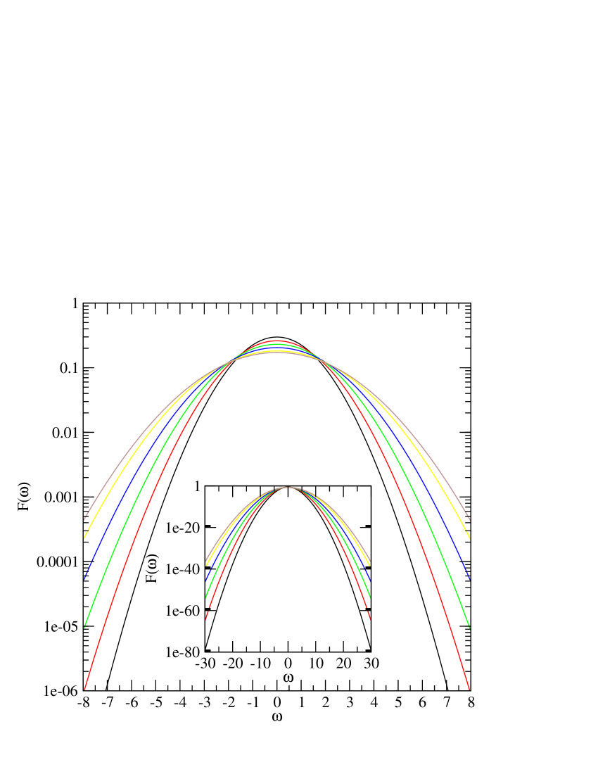
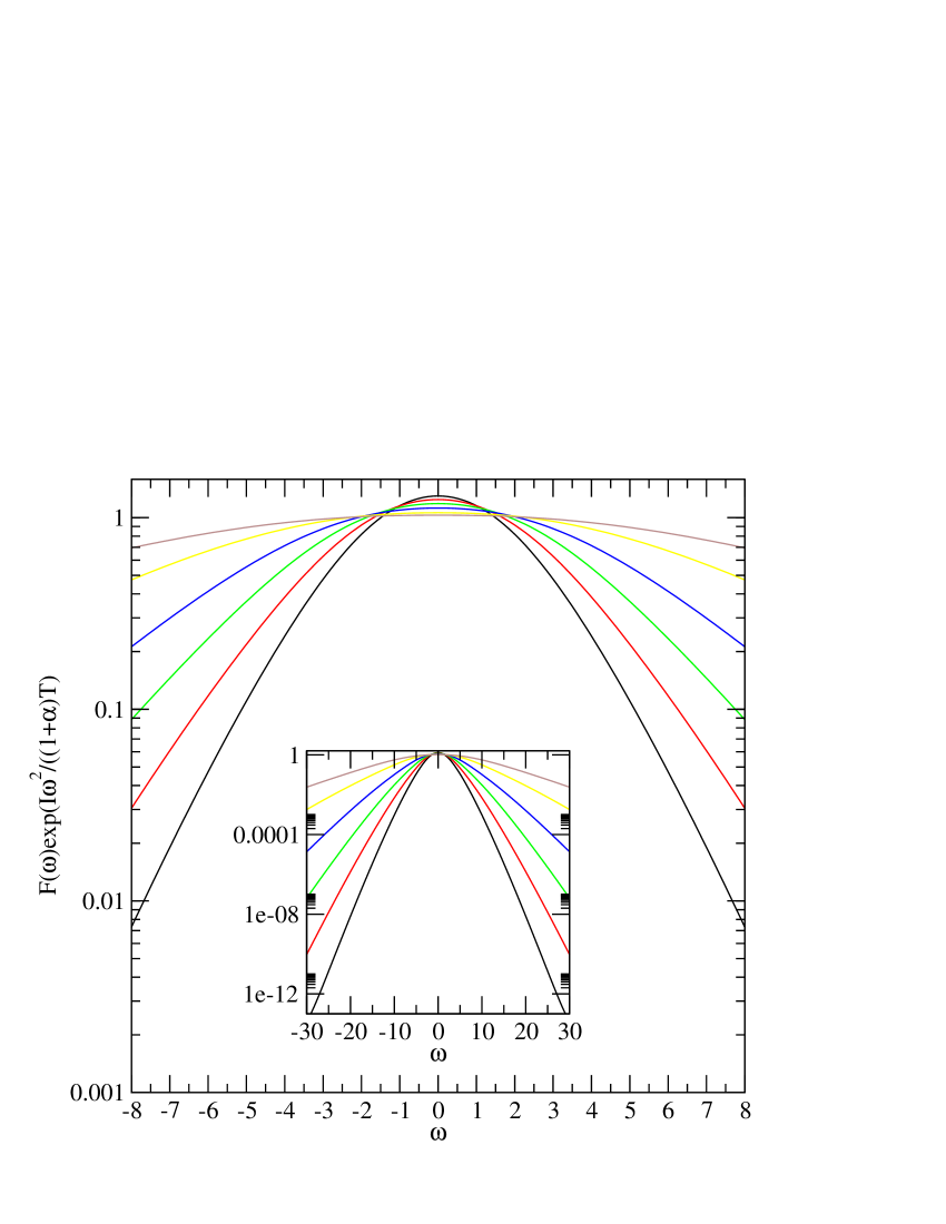
Figure 3: Same caption as Fig.2 for for $M/m=1$

IV Zero-mass limit

When both the mass of the needle and the coefficient of restitution are equal to zero, the Boltzmann equation, Eq.(II.2), can be solved exactly. Let us review the special characteristics of this limiting case. First, because of the zero mass of the tracer particle, the velocity of the bath particles never changes as the result of a collisions.In addition, the angular velocity of the needle has no memory of its pre-collisional value. This quantity is reset after each collision, acquiring instantaneously the value $v_{\perp}/\lambda$. By introducing the variable $v_{\perp}=(\lambda\omega)y$, Eq.(II.2) can be written as

$$\int_{-L/2}^{L/2}d\lambda\lambda^{2}\int dy|y|F\left(w\left(1+y\frac{(1+\alpha)m\lambda^{2}}{I+m\lambda^{2}}\right)\right)$$

$$\phi_{B}\left(\lambda\omega\left(1+y\frac{(\alpha m\lambda^{2}-I)}{I+m\lambda^{2}}\right)\right)$$

$$=F(\omega)\int_{-L/2}^{L/2}d\lambda\lambda^{2}\int dy|y-1|\phi_{B}(\lambda\omega y)$$ (20)

When $I=0$ and $\alpha=0$, this simplifies to

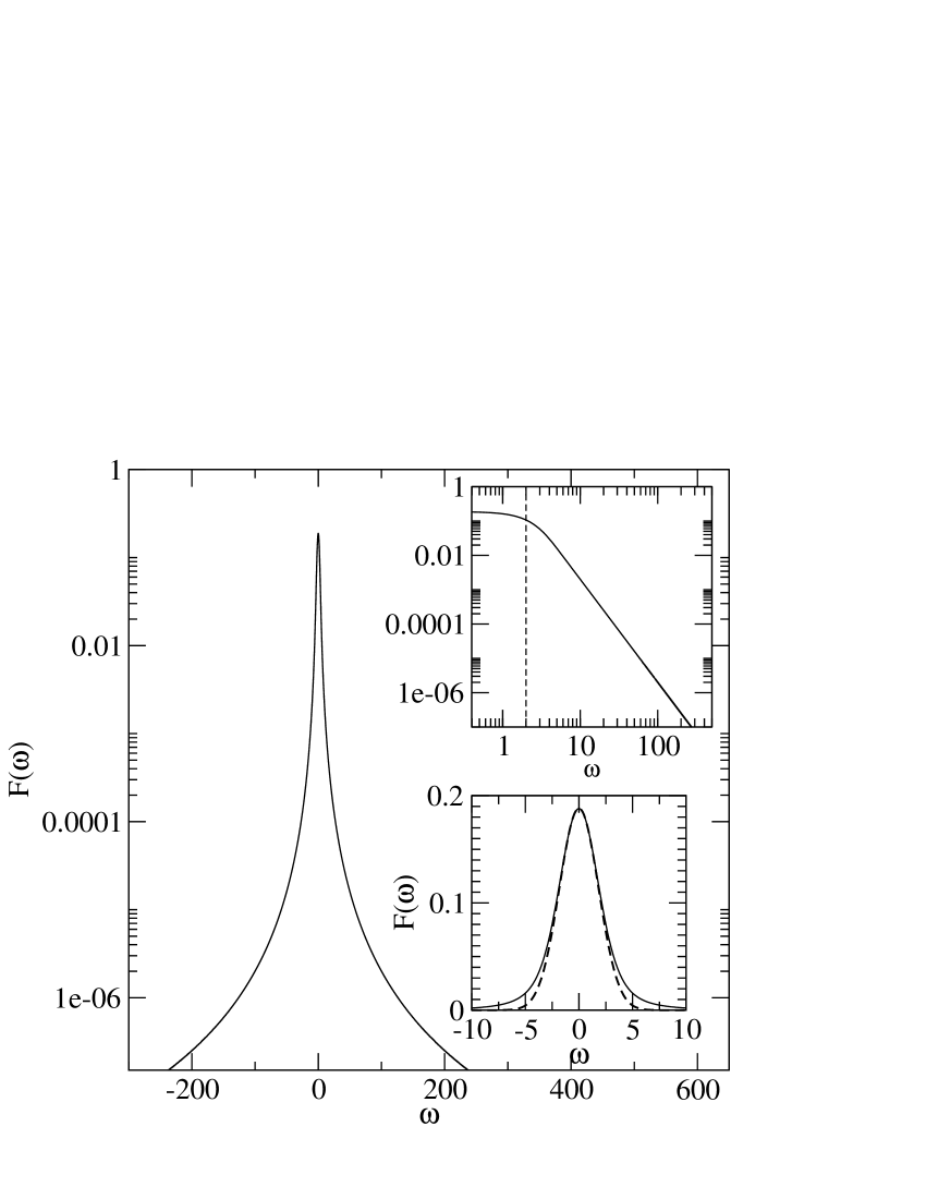
Figure 4: Log-linear plot $F(\omega)$ of the “zero mass” needle with $\omega_{c}=2$. The upper inset displays the log-log plot showing the power-law decay for sufficiently large $\omega$ values (the vertical dashed line corresponds to $\omega=\omega_{c}$). The lower inset is a log-log plot showing the gaussian behavior for $\omega<\omega_{c}$ (the dashed curve corresponds to the gaussian approximation)

$$\int_{-L/2}^{L/2}d\lambda\lambda^{2}\int dy|y|F\left(w\left(1+y\right)\right)\phi_{B}\left(\lambda\omega\right)$$

$$=F(\omega)\int_{-L/2}^{L/2}d\lambda\lambda^{2}\int dy|y+1|\phi_{B}(\lambda\omega y)$$ (21)

The exact solution $F(\omega)$ of Eq.(IV) is obtained by integrating the bath distribution $\phi_{B}(\lambda\omega)$ weighted by the position $\lambda$ of the point of impact:

$$F(\omega)=\int_{-L/2}^{L/2}d\lambda\left(\frac{2\lambda}{L}\right)^{2}\phi_{B}(\lambda\omega)$$ (22)

Note that this solution is independent of specific assumptions about the distribution of the bath particles. If we make the weak assumption that the second moment of the distribution $\phi_{B}(v)$ is finite, i.e. that the bath is characterized by a finite granular temperature, it can be shown that $F(\omega)$ decays algebraically as $\omega^{-3}$. The long tail of $F(\omega)$ arises from collisions near the center of the rotator that result in large angular velocities. It is worth noting that solutions of the Bolzmann equation with power-law decay exist for isotropic particles, but not with a thermalized bath of particlesBen-Naim and Machta (2005); Ben-Naim et al. (2005).

While the granular temperature of the bath particles is finite, that of the tracer is not well defined since its zero mass implies an infinite mean squared angular velocity. This difficulty is removed when the granular particle has a small, but finite mass (see below)

An explicit expression of the angular velocity distribution function $F(\omega)$ can be obtained when the bath particles have a Maxwellian velocity distribution, $\phi_{B}(v)=\sqrt{m/2\pi T}\exp(-mv^{2}/2T)$. In this case

$$F(\omega) =-\sqrt{\frac{1}{\pi}}\frac{\omega_{c}}{\omega^{2}}\exp\left(-\frac{\omega^{2}}{\omega_{c}^{2}}\right)+\frac{\omega_{c}^{2}}{2\omega^{3}}{\rm erf}\left(\frac{\omega}{\omega_{c}}\right)$$ (23)

where $\omega_{c}=\sqrt{8T/(mL^{2})}$ is a crossover frequency between two regimes. For $\omega>\omega_{c}$, $F(\omega)$ has a power-law behavior and for $\omega<\omega_{c}$, $F(\omega)\sim\exp(-3\omega^{2}/(5\omega_{c}^{2}))$ is gaussian (see Fig.4). It is important to note that when the power-law regime begins, the amplitude of $F(\omega)$ has only decreased by an order of magnitude compared to the maximum, $F(0)$.

An obvious question is whether the behavior just described persists when either $\alpha$ or $M/m$ is different from zero. Is the power law regime sustained in these cases?

We first consider the case where the mass ratio is maintained at zero, but the coefficient of restitution is allowed to take all values between $0$ and $1$. For $\alpha=1$ (elastic collisions) the solution of the Boltzmann equation is the expected Maxwell distribution:

$$F(\omega)=\sqrt{\frac{I}{2\pi T}}\exp\left(-\frac{I\omega^{2}}{2T}\right)$$ (24)

but the limit $I\to 0$ does not yield a probability distribution.

For $0<\alpha<1$ and $I=0$, we were unable to obtain an analytical solution and we investigated the behavior numerically with the method described above. Figure 5 shows the logarithm of the distribution function versus the angular velocity. As in the case $\alpha=0$, two distinct regimes characterize $F(\omega)$: a scaling regime for $\omega>\omega_{c}(\alpha)$, where $\omega_{c}(\alpha)$ is a cutoff which increases with $\alpha$ and a gaussian behavior at low frequencies.

Fig.5 shows that, in the power-law regime, while the amplitude of $F(\omega)$ decreases when $\alpha$ increases, the exponent of the power-law is independent of $\alpha$. It is possible to obtain this result analytically by means of an asymptotic analysis of the Boltzmann equation, Eq.(IV). Details of the calculation are given in Appendix B. The final result, for $M=0$ and $0<\alpha<1$, is

$$F(\omega)\sim\frac{4T(1+\alpha)}{mL^{2}(1-\alpha)\omega^{3}}.$$ (25)

Unlike the case where $\alpha=0$, the rotator has a memory of its previous angular velocity after a collision with a bath particle, $\omega^{*}=\alpha\omega+(1+\alpha)v_{\perp}/\lambda$. This memory effect can be very small when a bath particle collides near the center of the rotator (small $\lambda$), which explains why, for large angular velocities, the distribution function behaves similarly to the case $\alpha=0$.

The inset of Fig.5 displays $H(\omega)=F(\omega)\frac{mL^{2}(1-\alpha)}{4T(1+\alpha)}\omega^{3}$ versus $\omega$, showing that the asymptotic behavior is rapidly reached and that the numerical results agree accurately with Eq.(25).

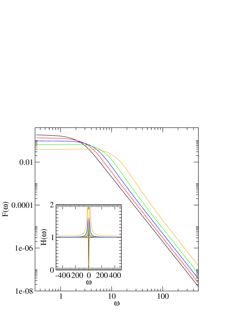
Figure 5: Log-Log plot of $F(\omega)$ of the “zero mass” needle with different values of the coefficient of restitution $\alpha=0,0.2,0.4,0.4,0.8$ from top to bottom. The inset shows the $\omega$-dependence of the rescaled function $H(\omega)=F(\omega)\frac{mL^{2}(1-\alpha)}{4T(1+\alpha)}\omega^{3}$ for $\omega_{c}=2$.

V Intermediate cases

We have considered in the preceding sections the two limiting cases of a large mass of the planar rotator (Brownian limit), where the angular velocity distribution function displays a gaussian-like behavior and a zero mass case where, surprisingly, a solution of the Boltzmann equation exists with a power-law decay of the distribution function. In this section, we investigate the intermediate case that corresponds to most physical situations.

We consider a planar rotator with a small but finite mass $0<M\ll m$. In Eq.(IV), since the integrand is an even function of $\lambda$, integration can be restricted to the positive abscissa. Moreover, the integration can be divided into two parts:

$$\int_{0}^{L/2}d\lambda=\int_{0}^{\epsilon}d\lambda+\int_{\epsilon}^{L/2}d\lambda$$ (26)

where $\epsilon>>\sqrt{\frac{I}{m}}$ (but $\epsilon$ being always small compared with $L/2$). For small angular velocities $\omega$, the contribution of the first integral vanishes, and performing a first-order expansion of the arguments of the integrand, one obtains

$$\int_{\epsilon}^{L/2}d\lambda F(\omega(1+y(1+\alpha)))\phi_{B}(\lambda(1+\alpha y))$$ (27)

which leads to the Boltzmann equation of the massless particle when $\epsilon\to 0$.

The existence of a finite mass allows for restoring a finite granular temperature. For small mass $M$, as shown above, the angular distribution function $F(\omega)$ has a power decay regime truncated at an upper $\omega_{c}^{(2)}$ where the gaussian begins. The granular temperature given by the product of the momentum of inertia times the second moment of the distribution function is dominated by the integral in the power-law regime.

$$T=\int d\omega F(\omega)I\omega^{2}$$

$$\simeq\int_{-\omega_{c}^{(2)}}^{\omega_{c}^{(2)}}I\frac{d\omega}{\omega}\sim I\ln(I)$$ (28)

which means that the granular temperature of small-mass planar rotator goes to zero when the mass decreases (even if the quadratic average of the angular velocity diverges logarithmically).

Fig.6 shows the distribution function for three small mass ratios $M/m=0.005,0.01,0.1$ with $\alpha=0$. As expected the low frequency distribution is well approximated by the massless distribution function. The inset shows that the range of the power-law decay decreases as the mass of the planar rotator increases. For large angular velocities, the distribution function resumes the gaussian behavior, $F(w)\sim\exp(-I\omega^{2}/((1+\alpha)T))$, irrespective of the needle-to-bath particle mass ratio.

In summary, the velocity distribution keeps memory of the massless solution up to second crossover angular velocity $\omega_{c}^{(2)}\sim\sqrt{2T/I}$. If the mass of the planar rotator is sufficiently small, one observes three successive regimes: first, a gaussian decay, second a power-law and finally a gaussian-like decay (sub-dominant terms are present).

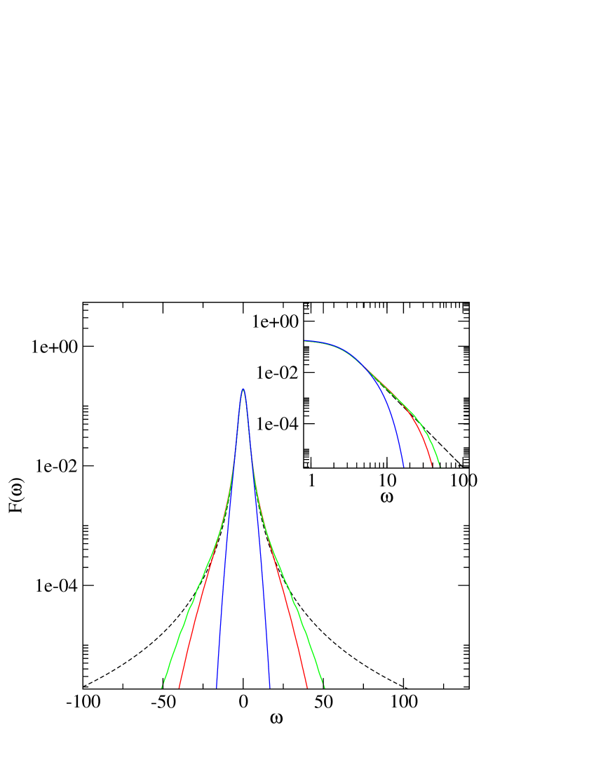
Figure 6: Log-Log plot of $F(\omega)$ for a needle with a mass $M/m=0.005,0.01,0.1$ (dashed curve corresponds to $M=0.0$). The inset shows the crossover between the power law and the gaussian-like asymptotic

When the masses of the planar rotator and a bath particle are comparable, the two crossover angular velocities merge and the power-law regime disappears. However, $F(\omega)$ may still deviate significantly from a gaussian. In order to show this we introduce the quantity

$$\eta=\frac{\langle\omega^{4}\rangle}{3\langle\omega^{2}\rangle^{2}}-1$$ (29)

which is zero for a gaussian distribution. Fig.7 displays $\eta$ as a function of the coefficient of restitution $\alpha$ for different masses $M/m=0.1,1,2,10$.

For the spherical tracer particle, the distribution function is a pure gaussian when the bath of particles is a gaussianMartin and Piasecki (1999). Deviations from the gaussian occur, however, in a mixture composed of granular particles of finite density immersed in a thermostat providing the energy via elastic collisions when this energy is redistributed within the granular component through inelastic encountersBiben et al. (2002). For anisotropic particles, our calculations show that deviations are present even in the limiting case of infinite dilution.

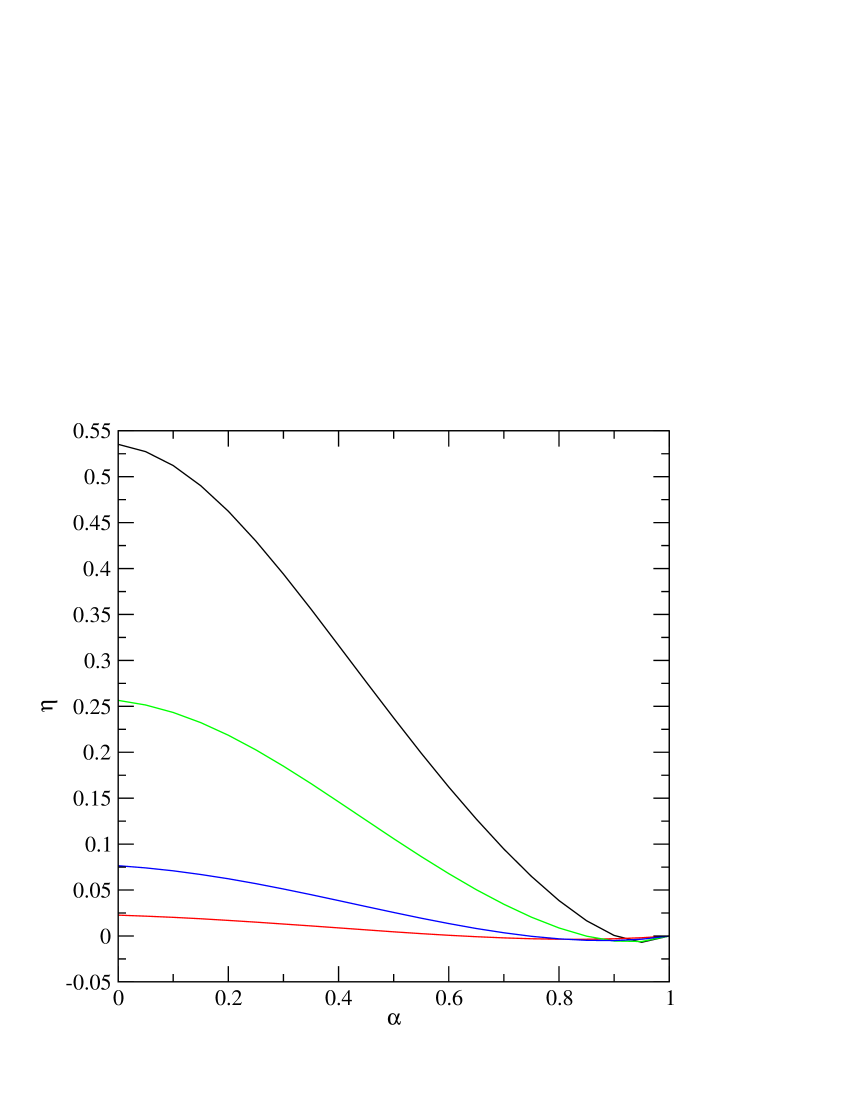
Figure 7: Deviations of the angular velocity distribution function from a gaussian for $M/m=0.1,1,2,10$, top to bottom.

VI Models with free or fixed center

The model of granular planar rotator with a free center in a thermalized bath has been previously investigated by two of usViot and Talbot (2004). In this model, the tracer particle has, in addition to the rotational one, two translational degrees of freedom.

By using an approximate theory, as well as numerical simulations of the Boltzmann equation, it was shown that the translational and rotational granular temperatures are both smaller than the bath temperature and also different from each other. In addition, the translational and rotational degrees of freedom are correlatedTalbot and Viot (2006).

In this section, we compare the rotational granular temperatures for the two models, all parameters being the same (mass, coefficient of restitution, bath temperature,…).

In order to obtain an analytical expression for the rotational temperature, we use a method originally proposed by Zippelius and colleagues that consists of calculating the second moment of the angular velocity of the Boltzmann equationHuthmann et al. (1999); Aspelmeier et al. (2001); Viot and Talbot (2004). In a stationary state, this quantity is constant, and by using an gaussian ansatz for $F(\omega)$

$$F(\omega)\propto\exp\left(\frac{-I{\bf\omega}^{2}}{2\overline{T}}\right),$$ (30)

one obtains a closed equation for the granular temperature $\overline{T}$ as a function of microscopic quantities:

$$\int_{0}^{1}dx\frac{\overline{T}}{T}x^{2}\frac{\sqrt{1+\frac{\overline{T}}{T}kx^{2}}}{1+kx^{2}} =\frac{1+\alpha}{2}\int_{0}^{1}dx\frac{x^{2}(1+\frac{\overline{T}}{T}kx^{2})^{3/2}}{(1+kx^{2})^{2}},$$ (31)

where

$$k=\frac{mL^{2}}{4I}$$ (32)

Details of the calculation are given in Appendix C. Eq. (31) is an implicit equation for $\overline{T}$, but, for a given value of $\alpha$ and of the mass ratio, it can be solved with standard numerical methods.

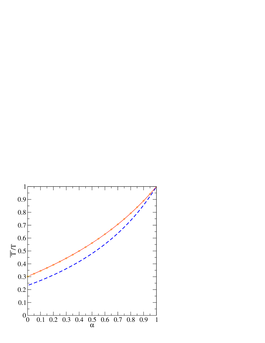
Figure 8: Effective granular temperature $\overline{T}$ as a function of the restitution of coefficient $\alpha$ for a fixed (full curve) and free rotator (dashed curve) in a bath of point particles. Circles correspond to the exact temperatures by computing the second moment of the distribution function obtained by the numerical resolution. The mass ratio is $M/m=1$

Fig 8 shows the variation of the rotational temperature with the normal coefficient of restitution for a mass ratio of $1$ for a fixed (solid curve) and free (dashed curve) planar rotator. The temperature is always higher when the center is fixed except in the case of elastic collisions, $\alpha=1$. The circles correspond to the “exact” temperatures obtained by computing the second moment of the distribution function $F(\omega)$, which shows that the above method provides accurate approximate results for estimating the granular temperatures.

We also consider the variation of the granular temperature with the mass ratio for a given value of the restitution coefficient: See Fig 9. It is easy to verify that in the Brownian limit, i.e. when the mass of the rotator is much larger of the particle mass, the granular temperature goes to a value, $(1+\alpha)/2$, that is independent of the mass ratio and, probably, the shape of particle. As the mass of the needle decreases, the difference between the rotational temperatures of the free and fixed planar rotator increases. For elastic systems, the rotational temperatures remain identical for the two different situations (free or fixed center of mass), but significant differences occur for a granular particle.

This phenomenon is more pronounced with varying mass ratio than with varying coefficient of restitution. Therefore, by monitoring the rotational motion of a granular needle in a bath of significantly heavier particles in two successive experiments (free and fixed center of mass), it should be possible to observe the absence of equipartition for a single particle.

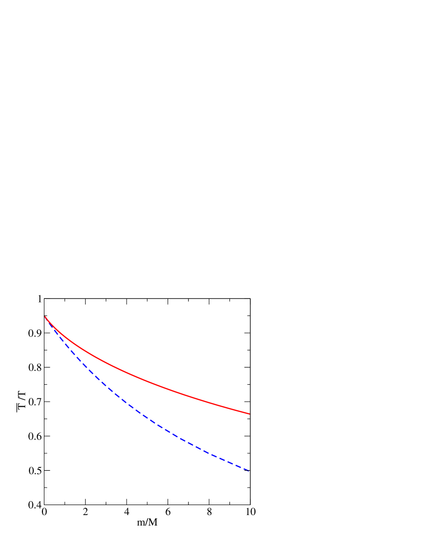
Figure 9: Effective granular temperature $\overline{T}$ as a function of the mass ratio $M/m$ for a fixed (full curve) and free rotator (dashed curve) in a bath of point particles. The coefficient of restitution is $\alpha=0.9$.

VII Conclusion

We have shown that the stationary angular velocity distribution of a planar rotator with a fixed center that collides inelastically with particles in a thermalized bath displays a variety of behavior as the mass of the rotator is changed. Starting from a quasi-gaussian regime when the rotator is much heavier than the bath particle, $F(\omega)$ shows significant deviations from the gaussian when the mass of the rotator is comparable to that of a bath particle. As the rotator mass decreases further, an intermediate power-regime also appears.

We believe that these features are not specific to this simple model, but are generic for all granular systems containing non-spherical particles. Furthermore, we expect that the non-gaussian character that is present in the idealized configuration of a thermalized bath will be amplified in in the presence of a granular (non-thermal) bath. Several experiments on intensely vibrated granular systems using high speed photographyFeitosa and Menon (2002, 2004), image analysis and particle trackingWildman et al. (2001); Wildman and Parker (2002) have shown that many quantities, including granular temperature and velocity profiles, can be precisely measured. As recent experimental studies have demonstrated, some of the same techniques can also be applied to granular rodsBlair et al. (2003); Volfson et al. (2004); Galanis et al. (2006); Lumay and Vandewalle (2004, 2006). We believe that the significant difference between the granular temperatures of a free and fixed rotator that we have identified (Fig 9) should be detectable using available experimental methods.

Appendix A Dimensionless Boltzmann equation

In order to consider the Brownian motion regime, it is convenient to introduce dimensionless variables $\Omega=\sqrt{I/k_{B}T}\omega$ and $u_{\perp}=\sqrt{m/k_{B}T}v_{\perp}$.

In terms of these variables the integrand in the Boltzmann equation (8) takes the form

$$F\left(\Omega+u_{\perp}\frac{(1+\alpha)\epsilon}{1+\epsilon^{2}}\right)\phi_{B}(\Omega\epsilon+u_{\perp}\frac{\alpha\epsilon^{2}-1}{1+\epsilon^{2}})$$

$$-F(\Omega)\phi_{B}(u_{\perp}+\epsilon\Omega)$$ (33)

where $\epsilon=\sqrt{m\lambda^{2}/I}=\sqrt{12m/M}\lambda/L$.

It is thus clear by inspection that the expansion of the dimensionless collision term (A) in powers of $\epsilon$ is equivalent to the expansion of the collision term (8) in powers of $\lambda$. Notice that keeping the variable $\Omega$ fixed when exploring the region of $m\ll M$ corresponds to the Brownian motion asymptotics, as then the rotational energy $I\omega^{2}$ is maintained at a fixed ratio with the thermal energy $k_{B}T$.

Appendix B Asymptotic behavior of the angular velocity distribution in the zero mass limit

Performing the change of variable $u=\omega(y+1)$ in the left-hand side of Eq.(IV) and $u=\omega y$ in the right-hand side, one obtains

$$\int_{-L/2}^{L/2}d\lambda\lambda^{2}\int du|u-\omega|F\left((1+\alpha)u-\alpha\omega\right)$$

$$\phi_{B}\left(\lambda((1-\alpha)\omega+\alpha u)\right)$$

$$=F(\omega)\int_{-L/2}^{L/2}d\lambda\lambda^{2}\int du|u-\omega|\phi_{B}(\lambda u)$$ (34)

When $|\omega|\to\infty$, one has

$$\int du|u-\omega|\phi_{B}(\lambda u)\sim\frac{|\omega|}{\lambda}$$ (35)

and therefore, the right-hand side of Eq.(B) becomes

$$F(\omega)\left(\frac{L}{2}\right)^{2}|\omega|$$ (36)

Performing a similar analysis for the right-hand side of Eq.(B), one gets the asymptotic relation of the Boltzmann equation (for the zero-mass limit)

$$F(\omega)\left(\frac{L}{2}\right)^{2}=\int_{-L/2}^{L/2}d\lambda\lambda^{2}\int duF\left((1+\alpha)u-\alpha\omega\right)$$

$$\phi_{B}\left(\lambda((1-\alpha)\omega+\alpha u)\right)$$ (37)

Let us introduce the Fourier transforms of the distribution functions $F(\omega)$ and $\phi_{B}(u)$ (with the convention $\hat{F}(k)=\int d\omega F(\omega)e^{-ikr}$). The right-hand-side of Eq.(B) can be expressed as

$$\int\frac{dk}{2\pi}\int\frac{dq}{2\pi}\int_{-L/2}^{L/2}d\lambda\lambda^{2}\hat{F}(k)\hat{\phi}_{B}(q)$$

$$\int due^{ik[(1+\alpha)u-\alpha\omega]}e^{iq\lambda[(1-\alpha)\omega+\alpha u]}$$ (38)

By using the property $\int dxe^{iax}=2\pi\delta(a)$, integration over $v$ in Eq.(B) can be carried out and one obtains

$$\int\frac{dq}{2\pi}\int_{-L/2}^{L/2}d\lambda\lambda^{2}\hat{F}\left(\frac{\lambda\alpha q}{1+\alpha}\right)\frac{\hat{\phi}_{B}(q)}{1+\alpha}e^{i\omega\left(\frac{\lambda q}{1+\alpha}\right)}$$ (39)

By taking the Fourier transform of Eq.(B) and by using Eq.(39), the asymptotic form of the Boltzmann equation becomes

$$\hat{F}(k)\left(\frac{L}{2}\right)^{2}=\hat{F}(\alpha k)\int_{-L/2}^{L/2}d\lambda|\lambda|\hat{\phi}_{B}\left(\frac{1+\alpha}{\lambda}q\right)$$ (40)

The integral of the right-hand side of Eq.(40) can explicitly performed

$$\int_{-L/2}^{L/2}d\lambda|\lambda|\hat{\phi}_{B}\left(\frac{1+\alpha}{\lambda}q\right) =\int_{0}^{1}d\mu\exp\left(-2\frac{(1+\alpha)^{2}k^{2}T}{\mu mL^{2}}\right)$$

$$=\exp\left(-2\frac{(1+\alpha)^{2}k^{2}T}{mL^{2}}\right)$$

$$-2\frac{(1+\alpha)^{2}k^{2}T}{mL^{2}}E_{i}\left(1,2\frac{(1+\alpha)^{2}k^{2}T}{mL^{2}}\right)$$ (41)

where $E_{i}(1,x)$ is the exponential integral. For small values of $k$, Eq.(B) behaves as

$$\int_{-L/2}^{L/2}d\lambda\lambda\hat{\phi}_{B}(\frac{1+\alpha}{\lambda}q)\simeq 1+4\frac{(1+\alpha)^{2}T}{mL^{2}}k^{2}\ln(|k|)$$ (42)

Inserting Eq.(42) in Eq.(40) yields

$$\hat{F}(k)\left(\frac{L}{2}\right)^{2}=\hat{F}(\alpha k)(1+4\frac{(1+\alpha)^{2}T}{mL^{2}}k^{2}\ln(|k|)$$ (43)

Iterating Eq.(43) and by using that $\hat{F}(k)=1$, one obtains that

$$\hat{F}(k)=1+\frac{1+\alpha}{1-\alpha}\frac{4T}{mL^{2}}k^{2}\ln(|k|)$$ (44)

The inverse Fourier transform of Eq.(44) leads to Eq.(25)

Appendix C Granular rotational temperature of the planar rotator with a gaussian approximation

By taking the second moment of Eq.(II.2), one obtains the following equation

$$\int_{-L/2}^{L/2}d\lambda\int v\int d\omega\theta(\omega\lambda-v)|v-\omega\lambda|F(\omega)\phi_{B}(v)\Delta\omega^{2}=0$$ (45)

where $\Delta\omega^{2}=\omega^{*2}-\omega^{2}$. This equation means that for a stationary state the second moment of the distribution is time independent, or in other words, that the loss of the rotational energy of the planar rotator induced by inelastic collisions is compensated on average by collisions with bath particles with higher velocities.

By using Eq.(6), the difference between the square angular velocities at a collision is given by

$$\Delta\omega^{2} =-\lambda(1+\alpha)\frac{{\bf V}.{\bf u}^{\perp}(\omega^{*}+\omega_{)}}{\frac{I}{m}+\lambda^{2}}$$

$$=-2\lambda(1+\alpha)\frac{{\bf V}.{\bf u}^{\perp}\omega}{\frac{I}{m}+\lambda^{2}}+\lambda^{2}(1+\alpha)^{2}\frac{({\bf V}.{\bf u}^{\perp})^{2}}{\left(\frac{I}{m}+\lambda^{2}\right)^{2}}.$$ (46)

Introducing the dimensionless vectors

$${\bf s}= (s_{x},s_{y})$$

$$=\left(\sqrt{\frac{m}{2T}}v,\sqrt{\frac{I}{2\overline{T}}}\omega\right)$$ (47)

and

$${\bf G}= (G_{x},G_{y})$$

$$=\left(\sqrt{\frac{2T}{m}},\sqrt{\frac{2\overline{T}}{I}}\lambda\right)$$ (48)

Therefore the scalar product ${\bf G}.{\bf s}$ gives

$${\bf G}.{\bf s}=v-\omega\lambda$$ (49)

Eq.(45) can be expressed as

$$\int_{-L/2}^{L/2}d\lambda\int d{\bf s}\exp(-{\bf s}^{2})\theta(-{\bf G}.{\bf s})|{\bf G}.{\bf s}|$$

$$\left[-\frac{2\lambda(1+\alpha){\bf G}.{\bf s}}{\frac{I}{m}+\lambda^{2}}\sqrt{\frac{2\overline{T}}{I}}s_{y}+\frac{\lambda^{2}(1+\alpha)^{2}({\bf G}.{\bf s})^{2}}{\left(\frac{I}{m}+\lambda^{2}\right)^{2}}\right]=0$$ (50)

Let us define a new coordinate systemAspelmeier et al. (2001) where the y-axis is parralel to ${\bf G}$: units vectors are denoted $({\bf e}_{1},{\bf e}_{2})$ whereas the unit vectors of the original system $({\bf e}_{x},{\bf e}_{y})$. It follows that ${\bf G}=|{\bf G}|{\bf e}_{1}$ and therefore one can write that

$${\bf G}{\bf e}_{1}{\bf e}_{y}=|{\bf G}|{\bf e}_{x}=G_{x}$$ (51)

Inserting Eq.(51) in Eq.(C) allows for performing standard gaussian integrals and finally one obtains Eq.(31)

References

- Goldhirsch (2003) I. Goldhirsch, Annu. Rev. Fluid. Mech. 35, 267 (2003).
- Brilliantov and Pöschel (2004) N. V. Brilliantov and T. Pöschel, Kinetic theory of granular gases (Oxford University Press, 2004).
- Zippelius (2006) A. Zippelius, Physica A 369, 143 (2006).
- Wildman and Parker (2002) R. D. Wildman and D. J. Parker, Phys. Rev. Lett. 88, 064301 (2002).
- Feitosa and Menon (2002) K. Feitosa and N. Menon, Phys. Rev. Lett. 88, 198301 (2002).
- Martin and Piasecki (1999) P. A. Martin and J. Piasecki, Europhys. Lett 46, 613 (1999).
- Huthmann et al. (1999) M. Huthmann, T. Aspelmeier, and A. Zippelius, Phys. Rev. E 60, 654 (1999).
- Barrat and Trizac (2002) A. Barrat and E. Trizac, Granul. Matter 4, 57 (2002).
- Brey et al. (1999) J. J. Brey, D. Cubero, and M. J. Ruiz-Montero, Phys. Rev. E 59, 1256 (1999).
- Rouyer and Menon (2000) F. Rouyer and N. Menon, Phys. Rev. Lett. 85, 3676 (2000).
- Atwell and Olafsen (2005) J. Atwell and J. S. Olafsen, Phys. Rev. E 71, 062301 (2005).
- Pöschel and Brilliantov (2003) T. Pöschel and N. Brilliantov, Granular Gas Dynamics (Springer, Berlin, 2003).
- Viot and Talbot (2004) P. Viot and J. Talbot, Phys. Rev. E 69, 051106 (2004).
- Gomart et al. (2005) H. Gomart, J. Talbot, and P. Viot, Phys. Rev. E 71, 051306 (2005).
- Piasecki and Viot (2006) J. Piasecki and P. Viot, Europhys. Lett 74, 1 (2006).
- Biben et al. (2002) T. Biben, P. A. Martin, and J. Piasecki, Physica A 310, 308 (2002).
- Montanero and Santos (2000) J. M. Montanero and A. Santos, Granular Matter 2, 53 (2000).
- Ben-Naim and Machta (2005) E. Ben-Naim and J. Machta, Phys. Rev. Lett. 94, 138001 (2005).
- Ben-Naim et al. (2005) E. Ben-Naim, B. Machta, and J. Machta, Phys. Rev. E 72, 021302 (2005).
- Talbot and Viot (2006) J. Talbot and P. Viot, J. Phys. A. Math. Gen. 39, 10947 (2006).
- Aspelmeier et al. (2001) T. Aspelmeier, T. M. Huthmann, and A. Zippelius, Granular Gases (Springer, Berlin, 2001), chap. Free cooling of particles with rotational degrees of freedom, p. 31.
- Feitosa and Menon (2004) K. Feitosa and N. Menon, Phys. Rev. Lett. 92, 164301 (2004).
- Wildman et al. (2001) R. D. Wildman, J. M. Huntley, and D. J. Parker, Phys. Rev. Lett. 86, 3304 (2001).
- Blair et al. (2003) D. L. Blair, T. Neicu, and A. Kudrolli, Phys. Rev. E 67, 031303 (2003).
- Volfson et al. (2004) D. Volfson, A. Kudrolli, and L. S. Tsimring, Phys. Rev. E 70, 051312 (2004).
- Galanis et al. (2006) J. Galanis, D. Harries, D. L. Sackett, W. Losert, and R. Nossal, Phys. Rev. Lett. 96, 028002 (2006).
- Lumay and Vandewalle (2004) G. Lumay and N. Vandewalle, Phys. Rev. E 70, 051314 (2004).
- Lumay and Vandewalle (2006) G. Lumay and N. Vandewalle, Phys. Rev. E 74, 021301 (2006).