Dynamical localization of matter wave solitons in managed barrier potentials

Abstract

The bright matter wave soliton propagation through a barrier with a rapidly oscillating position is investigated. The averaged over rapid oscillations Gross-Pitaevskii (GP) equation is derived. It is shown that the soliton is dynamically trapped by the effective double-barrier. The analytical predictions for the soliton effective dynamics is confirmed by the numerical simulations of the full GP equation.

I Introduction

The tunneling of quantum particles is one of the fundamental problems of quantum mechanics Landauer . In connection with this problem, the propagation of matter wave packets through different types of potentials has recently attracted a lot of attention. In particular it is interesting to study the transmission through time-dependent barriers. Indeed, experiments with dynamical tunneling of cold atoms in time-dependent barriers of the multiplicative form $f(t)V(x)$ show the possibility for the tunneling period control Hensinger ; Steck . The theory is developed for linear wavepackets in Ref. Averbukh . Soliton propagation through such a barrier is investigated in Ref. AG . Another interesting problem is to consider a barrier with a rapidly oscillating position, i.e. a potential of the form $V(x-f(t))$. In the linear regime of propagation resonant effects are exhibited in the transmission process through an oscillating barrier Chiofalo ; Embriaco . It is therefore relevant to investigate the propagation of a nonlinear wave packet through an oscillating barrier. We consider this problem for a bright matter wave soliton in an attractive Bose-Einstein condensate (BEC) in the presence of a barrier potential with an oscillating position. Such a barrier can be achieved by using a laser beam with a blue-detuned far-off-resonant frequency. This generates a repulsive potential and the laser sheet plays the role of a mirror for cold atoms. Such a laser sheet has been used to study the bouncing of a BEC cloud off a mirror Bongs . By moving the position of the mirror we obtain an oscillating barrier.

In this work we will study the dynamical trapping of soliton in BEC with a rapidly oscillating barrier potential. The averaged over rapid oscillations Gross-Pitaevskii (GP) equation will be derived. Applying a variational approach to this equation, we will analyze the conditions for soliton trapping by the effective potential. The analytical predictions are checked by numerical simulations of the full GP equation.

II The averaged Gross-Pitaevskii equation

The BEC wavefunction $\psi$ in a quasi one-dimensional geometry is described by the GP equation

$$i\hbar\psi_{T}+\frac{\hbar^{2}}{2m}\psi_{XX}-V_{p}(X-f_{p}(T),T)\psi-g_{1D}|\psi|^{2}\psi=0,$$

where $V_{p}(X,T)$ is a barrier potential. Here $g_{1D}=2\hbar a_{s}\omega_{\perp}$ is the one-dimensional mean field nonlinearity constant, $a_{s}$ is the atomic scattering length, $\omega_{\perp}$ is the transverse oscillator period, and $a_{\perp}=\sqrt{\hbar/(m\omega_{\perp})}$ is the transverse oscillator length. Below we consider the case of BEC with attractive interactions, i.e. $a_{s}<0$. To avoid collapse in the attractive BEC, the condition $|a_{s}|N/a_{\perp}<0.67$ should be satisfied, with $N$ the number of atoms. The barrier potential has an oscillating position described by the zero-mean time-periodic function $f_{p}(T)$ with period $T_{p}$. We consider the case of a fast-moving potential in the sense that $\varepsilon:=\omega_{\perp}T_{p}\ll 1$. We also allow the barrier potential profile $V_{p}(X,T)$ to vary slowly in time, i.e. with a rate smaller than $\omega_{\perp}$. Introducing the standard dimensionless variables

$$x=\frac{\sqrt{2}X}{a_{\perp}},\ \ \ t=\omega_{\perp}T,\ \ \ u=\sqrt{|a_{s}|}\psi,\ \ \ V=\frac{V_{p}}{\hbar\omega_{\perp}},$$

we obtain the GP equation with fast moving potential

$$iu_{t}+u_{xx}-V\left(x-f(\frac{t}{\varepsilon}),t\right)u+2|u|^{2}u=0,$$ (1)

where

$$f(t)=\frac{\sqrt{2}}{a_{\perp}}f_{p}(T_{p}t)$$

is a periodic function with period $1$ and mean $0$. The small parameter $\varepsilon$ describes the fast oscillation period in the dimensionless variables. We look for the solution in the form

$$u(x,t)=u^{(0)}(x,t,\frac{t}{\varepsilon})+\varepsilon u^{(1)}(x,t,\frac{t}{\varepsilon})+\varepsilon^{2}u^{(2)}(x,t,\frac{t}{\varepsilon})+\cdots$$ (2)

where $u^{(0)}$, $u^{(1)}$, $\ldots$ are periodic in the argument $\tau=t/\varepsilon$. We substitute this ansatz into Eq. (1) and collect the terms with the same powers of $\varepsilon$. We obtain the hierarchy of equations:

$$iu^{(0)}_{\tau}=0,$$ (3)

$$iu^{(0)}_{t}+u^{(0)}_{xx}-V\left(x-f(\tau),t\right)u^{(0)}+2|u^{(0)}|^{2}u^{(0)}=-iu^{(1)}_{\tau},$$ (4)

$$iu^{(1)}_{t}+u^{(1)}_{xx}-V\left(x-f(\tau),t\right)u^{(1)}+4\bigl{(}u^{(0)}\bigr{)}^{2}\overline{u^{(1)}}+2\bigl{|}u^{(0}\bigr{|}^{2}u^{(1)}=-iu^{(2)}_{\tau}.$$ (5)

The first equation (3) shows that the leading-order term $u^{(0)}$ does not depend on $\tau$. The second equation (4) gives the compatibility equation for the existence of the expansion (2):

$$iu^{(0)}_{t}+u^{(0)}_{xx}-\left<V\left(x-f(\cdot),t\right)\right>u^{(0)}+2|u^{(0)}|^{2}u^{(0)}=0,$$

where $\left<\cdot\right>$ stands for an average in $\tau$. Denoting

$$V_{\rm eff}(x)=\int_{0}^{1}V\left(x-f(\tau),t\right)d\tau$$ (6)

we obtain the averaged GP equation

$$iu_{t}+u_{xx}-V_{\rm eff}(x,t)u+2|u|^{2}u=0.$$ (7)

The equation (5) allows us to compute the first order correction, whose amplitude is of order $\varepsilon$.

If, for example, $f(\tau)=a\sin(2\pi\tau)$, then a straightforward calculation shows that

$$V_{\rm eff}(x,t)=K_{\rm eff}*V(x,t),$$ (8)

where $*$ stands for the convolution product (in $x$) and $K_{\rm eff}$ is given by

$$K_{\rm eff}(x)=\frac{1}{\pi}\frac{1}{\sqrt{a^{2}-x^{2}}}{\bf 1}_{(-a,a)}(x).$$ (9)

If, moreover, $V(x,t)$ is a delta-like potential centered at a position $x_{0}(t)$ that moves slowly in time, then

$$V_{\rm eff}(x,t)=K_{\rm eff}(x-x_{0}(t))$$

is a moving double-barrier potential. By this way, one can generate a moving trap potential to manage the soliton position.

III Variational approach for the soliton motion

In absence of effective potential $V_{\rm eff}=0$ the NLS equation (7) supports soliton solutions of the form

$$u_{0}(x,t)=2\nu\frac{e^{i2\mu(x-x_{s}(t))+4i(\mu^{2}+\nu^{2})t}}{\cosh[2\nu(x-x_{s}(t))]}$$

with $x_{s}(t)=x_{s}(0)+4\mu t$. In the presence of a stationary potential $V_{\rm eff}(x)$, the soliton dynamics can be studied by perturbation techniques. Applying the first-order perturbed Inverse Scattering Transform theory Karpman , we obtain the system of equations for the soliton amplitude and velocity

$$\frac{d\nu}{dt}=0,\ \ \ \ \ \ \frac{d\mu}{dt}=-\frac{1}{4\nu}W_{\nu}^{\prime}(x_{s}),\ \ \ \ \ \ \frac{dx_{s}}{dt}=4\mu,$$

where the prime stands for a derivative with respect to $x$ and $W_{\nu}$ has the form

$$W_{\nu}(x) = \nu\int_{-\infty}^{\infty}\frac{1}{\cosh^{2}(z)}V_{\rm eff}\bigl{(}x-\frac{z}{2\nu}\bigr{)}dz$$

$$= K_{\nu}*V_{\rm eff}(x)\,,$$ (10)

$$K_{\nu}(x) = \frac{2\nu^{2}}{\cosh^{2}(2\nu x)}\,.$$ (11)

Therefore, we can write the effective equation describing the dynamics of the soliton center as a quasi-particle moving in the effective potential $W_{\nu_{0}}$:

$$\nu_{0}\frac{d^{2}x_{s}}{dt^{2}}=-W_{\nu_{0}}^{\prime}(x_{s}),$$ (12)

where $4\nu_{0}$ is the mass (number of atoms) of the initial soliton. This system has the integral of motion

$$\frac{\nu_{0}}{2}\left(\frac{dx_{s}}{dt}\right)^{2}+W_{\nu_{0}}(x_{s})=8\nu_{0}\mu_{0}^{2},$$ (13)

where $4\mu_{0}$ is the velocity of the initial soliton. Note that this approach gives the same result as the adiabatic perturbation theory for solitons that is a first-order method as well. This adiabatic perturbation theory was originally introduced for optical solitons kivshar89 ; Abd93 and it was recently applied to matter wave solitons kevrekidis .

The quasi-particle effective potential $W_{\nu}$ is given by

$$W_{\nu}(x)=(K_{\nu}*K_{\rm eff})*V(x).$$

In the case where $f(\tau)=a\sin(2\pi\tau)$, the kernel $K_{\rm eff}$ is given by (9) and the Fourier transform of the quasi-particle potential has the explicit form

$$\hat{W}_{\nu}(k)=\frac{\pi kJ_{0}(ka)}{2\sinh(\frac{\pi k}{4\nu})}\hat{V}(k)\,,$$

where $\hat{V}$ is the Fourier transform of the reference potential $V$. The effective quasi-particle potential is plotted in Fig. 1 for a Gaussian barrier potential $V$. The potential $W_{\nu}$ has a local minimum at $x=0$ between two global maxima that are close to $x=\pm a$. The trap amplitude is

$$\Delta W_{\nu}=\max_{x}W_{\nu}(x)-W_{\nu}(0).$$

Let us consider an input soliton at $x=0$ with parameters $(\nu_{0},\mu_{0})$. If the initial soliton velocity is large enough, then the soliton escapes the trap. There is a critical value $\mu_{c}$ for the initial soliton velocity parameter $\mu_{0}$ defined by

$$\mu_{c}^{2}=\frac{\Delta W_{\nu_{0}}}{8\nu_{0}}$$

that determines the type of motion:
- If $|\mu_{0}|<\mu_{c}$ then the soliton is trapped. Its motion is oscillatory between the positions $\pm x_{f}$ defined by

$$W_{\nu_{0}}(x_{f})-W_{\nu_{0}}(0)=8\nu_{0}^{2}\mu_{0}^{2}$$ (14)

- If $|\mu_{0}|>\mu_{c}$, then the soliton motion is unbounded. It escapes the trap and reaches the asymptotic velocity parameter $\mu_{a}$ given by

$$\mu_{a}^{2}=\frac{W_{\nu_{0}}(0)}{8\nu_{0}}+\mu_{0}^{2}$$ (15)

which shows that the transmitted soliton velocity is larger than the initial soliton velocity.

As we shall see in the numerical simulations, if the initial soliton parameters are close to the critical case $|\mu_{0}|\sim\mu_{c}$, then radiation effects become non-negligible. The construction of an efficient trap requires to generate a barrier potential $V$ that is high enough so that $\Delta W_{\nu_{0}}$ is significantly larger than $8\nu_{0}^{2}\mu_{0}$.

Finally, if the potential $V$ is not stationary but has an explicit time-dependence, such as a drift, then the adiabatic equations derived in this section still hold true if the time-dependence is slow enough.

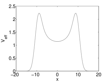
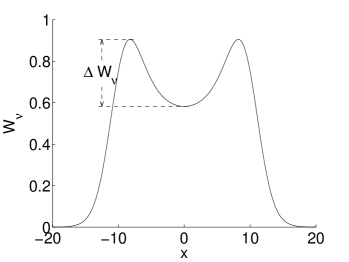
Figure 1: Effective potentials $V_{\rm eff}(x)$ for the averaged equation (7) and $W_{\nu}(x)$ for the quasi-particle motion (12). Here $\nu=0.25$, $V(x)=10\exp(-x^{2}/4)$, and $f(\tau)=10\sin(2\pi\tau)$.

IV Numerical simulations and experimental predictions

In this section we show the motion of a soliton with initial parameters $\nu_{0}=\mu_{0}=0.25$ (the soliton velocity is $1$). The reference barrier potential is $V(x)=10\exp(-x^{2}/4)$. Note that in this case, $\Delta W_{\nu_{0}}\simeq 0.323$ and $\mu_{c}\simeq 0.4$. Therefore, the quasi-particle approach predicts trapping.

In Fig. 2 the modulated potential is $V[x-10\sin(50t)]$ (stationary trap). Here $\varepsilon=2\pi/50\simeq 0.126$ and we check by full numerical simulations of the GP equation (1) that $\varepsilon$ is small enough to ensure the validity of the theoretical predictions based on the averaged GP equation (7). We plot the soliton profile and the soliton mass, which shows that radiative effects are very small. We also compare the soliton motion obtained by the numerical simulations with the one predicted by the quasi-particle approach, which shows very good agreement.

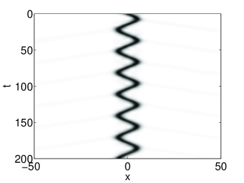
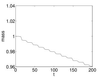
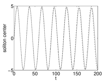
Figure 2: Soliton profile in a narrow trap $V[x-10\sin(50t)]$ (left picture). Mass decay (right picture). Bottom picture: Soliton motion predicted by the quasi-particle approach (dashed) and observed in the numerical simulations (solid).

In Fig. 3 the modulated potential is $V[x-10\sin(50t)-0.25t]$ (moving trap, with velocity $0.25$). We plot the soliton profile and the soliton mass, which shows that radiative effects are very small.

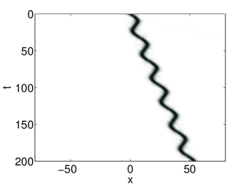
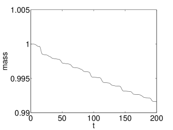
Figure 3: Soliton profile in a narrow moving trap $V[x-10\sin(50t)-0.25t]$ (left picture). Mass decay (right picture).

In Fig. 4 the modulated potential is $V[x-10\sin(50t)+0.25t]$ (moving trap, with velocity $-0.25$)). Radiation effects are small, but not completely negligible. It can be seen that some radiation is transmitted through the edges of the effective double-barrier trap. We then double the potential amplitude and consider $2V[x-10\sin(50t)+0.25t]$. The new simulation is shown in Fig. 5, where radiation effects are seen to be negligible.

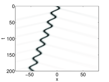
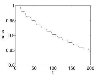
Figure 4: Soliton profile in the moving trap $V[x-10\sin(50t)+0.25t]$ (left picture). Mass decay (right picture).

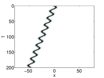
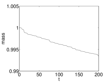
Figure 5: Soliton profile in the moving trap $2V[x-10\sin(50t)+0.25t]$ (left picture). Mass decay (right picture).

In Fig. 6 we show the motion of a soliton with initial parameters $\nu_{0}=0.25$ and $\mu_{0}=0.5$ (the soliton velocity is $2$). Since we have $\Delta W_{\nu_{0}}\simeq 0.323$ and $\mu_{c}=0.4$, the quasi-particle approach predicts unbounded motion. The results of the numerical simulations confirm this prediction. We can observe that half the initial soliton mass is transmitted through the effective barrier during the first interaction, and the transmitted soliton has a velocity that is larger than $4\mu_{0}$.

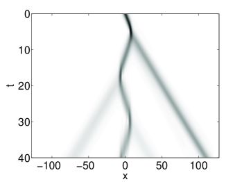
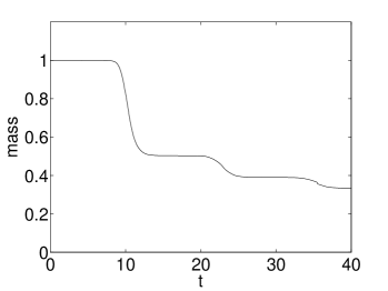
Figure 6: Soliton profile in the stationary trap $V[x-10\sin(50t)]$ (left picture). Mass decay (right picture). Here the initial velocity parameter is $\mu_{0}=0.5$.

Let us estimate the typical values of the parameters for an experimental configuration. We consider the case of a condensate with ⁷Li atoms in the a cigar-shaped trap potential with $\omega_{\perp}=2\pi\times 1$ kHz. In this case, $\varepsilon=2\pi/50$ corresponds to $1/T_{p}=50$ kHz. The barrier height is $V_{0}=10\hbar\omega_{\perp}$. The number of atoms can be taken as $N\sim 10^{3}$ for the scattering length $a_{s}=-0.2$ nm. The transverse oscillator length is $a_{\perp}=1.2~{}\mu$m, so the barrier width is $d\simeq 2~{}\mu$m and the oscillations amplitude of the barrier position is $L\simeq 10~{}\mu$m. The velocity is normalized by the sound velocity which is $c\simeq 4$ mm/s, so the soliton velocity parameter $\mu_{0}=0.25$ corresponds to a velocity equal to $c$.

V Conclusion

In conclusion we have studied the propagation of a bright matter wave soliton through a barrier potential with rapidly oscillating position. We have shown that the soliton can be dynamically trapped by such a potential. It would be interesting to extend this model to the case of oscillating barrier and standing well. In this case the effective potential will have the form of two barriers separated by a well. Applying the results obtained in Ref. Azbel we can expect for the transmission of the nonlinear matter waves such phenomena as the instability and quantum turbulence on the time scales of the quantum dwell time in the well. Another physically relevant system is the rapidly oscillating barrier in the well. The effective potential in this case simulates a heterostructure and effective nonlinearities can exhibit chaotic dynamics in the tunneling process Jona .

In the case of a well with rapidly oscillating position the effective potential will have a double-well form. In such a configuration we can expect the existence of dynamically induced macroscopic quantum tunnelling and localization phenomena, i.e. dynamically generated bosonic Josephson junction. These problems require of a separate investigation.

References

- (1) R. Landauer and Th. Martin, Rev. Mod. Phys. 66, 217 (1994).
- (2) W. K. Hensinger et al., Nature 412, 52 (1993).
- (3) D. A. Steck, W. H. Oskay, and H. G. Raizen, Science, 293, 274 (2001).
- (4) V. Averbukh, S. Osovski, and N. Moiseyev, Phys. Rev. Lett. 89, 253201 (2002).
- (5) F. Kh. Abdullaev and R. Galimzyanov, J. Phys. B 36, 1099 (2003).
- (6) M. L. Chiofalo, M. Artoni, and G. C. La Rocca, New Jour. Phys. 5, 78.1 (2003).
- (7) D. Embriaco, M. L. Chiofalo, M. Artoni, and G. L. La Rocca, J. Opt. B: Quant. Sem. Opt. 7, S59 (2005).
- (8) K. Bongs et al., Phys. Rev. Lett. 83, 3577 (1999).
- (9) M. Ya. Azbel , Phys. Rev. B 59, 8049 (1999).
- (10) G. Jona-Lasinio, C. Presilla, and F. Capasso, Phys. Rev. Lett. 68, 2269 (1992).
- (11) V. I. Karpman, Phys. Scr. 20, 462 (1979).
- (12) Yu. S. Kivshar and B. A. Malomed, Rev. Mod. Phys. 61, 763 (1989).
- (13) F. Kh. Abdullaev, S. A. Darmanyan, and P. K. Khabibullaev, Optical Solitons, Springer, Heidelberg, 1993.
- (14) G. Theocharis , P. Schmelcher, P. G. Kevrekidis, and D. J. Frantzeskakis, Phys. Rev. A 72, 033614 (2005).