Magnetization of concentrated polydisperse ferrofluids: Cluster expansion

Abstract

The equilibrium magnetization of concentrated ferrofluids described by a system of polydisperse dipolar hard spheres is calculated as a function of the internal magnetic field using the Born–Mayer or cluster expansion technique. This paper extends the results of Phys. Rev. E 62, 6875 (2000) obtained for monodisperse ferrofluids. The magnetization is given as a power series expansion in two parameters related to the volume fraction and the coupling strength of the dipolar interaction, respectively.

I Introduction

Ferrofluids R85 are suspensions of ferromagnetic particles of about 10 nm diameter in a carrier fluid. The particles are stabilized against aggregation by coating with polymers or by electrostatic repulsion of charges brought on their surface. As long as the concentration of the particles is low, the equilibrium magnetization of a ferrofluid is that of an ideal paramagnetic gas. In highly concentrated ferrofluids on the other hand, the magnetization is influenced by effects of particle–particle interactions.

We studied these effects for ferrofluids that are described by a system of identical dipolar hard spheres in HL , from now on referred to as paper I. In that paper we used the technique of the Born–Mayer or cluster expansion technique to evaluate the equilibrium magnetization as a series expansion in terms of the volume fraction $\phi=N\pi D^{3}/6V$, and a dipolar coupling parameter $\epsilon=m^{2}/4\pi\mu_{0}kT$, with $N/V$ being the particle density, and $D$ and $m$ being the common hard sphere diameter and magnetic moment of the particles, respectively.

However, real ferrofluids are polydisperse, i. e. the particles vary in size and magnetic moment. This property has a strong influence on the equilibrium magnetization, for concentrated as well as for dilute fluids. The goal of this paper is to generalize the findings of paper I to include the effects of polydispersity.

The linear response problem of determining the static initial susceptibility $\chi$ of a mixture of dipolar hard spheres was investigated already for the equivalent electric case in the framework of integral theories: The mean spherical model W71 was extended to binary or multicomponent mixtures AD73 ; IB74 ; HS78 ; FHI79 ; RH81 ; CB86 . The reference hypernetted chain method FP84 was also applied to bidisperse systems LL87 ; LL89 . Recently KS02 , the mean spherical model was used within the algebraic perturbation theory K99 , however without leading to new results for the initial susceptibility. The mean spherical model was also extended to polydisperse ferrofluids in arbitrary high fields SPMS90 ; ML90 . Another theory dealing with arbitrary fields is the high temperature approximation BI92 . A variant of this theory was proposed in PML96 and extended in IK01 .

Our calculation follows closely that of paper I. Therein the application of the cluster expansion technique to a monodisperse system of dipolar hard spheres resulted in an expression for the magnetization $M$ that can be put into the form

$$M=M_{\text{sat}}\sum_{m=0}^{\infty}\sum_{n=0}^{\infty}\phi^{m}\epsilon^{n}L_{m,n}(\alpha)\;\;,$$ (1)

where $M_{\text{sat}}$ is the saturation magnetization of the fluid. The functions $L_{m,n}(\alpha)$ were given explicitly in terms of analytic expressions in the dimensionless magnetic field $\alpha$. We calculated $L_{2,2}(\alpha)$ and some of the $L_{1,n}(\alpha)$. Lower orders vanish, except for the Langevin function $L_{0,0}(\alpha)$.

In the polydisperse case discussed here the parameters $\phi$, $\epsilon$ and $\alpha$ are replaced by more generally defined quantities $\overline{\phi}$, $\overline{\epsilon}$ and $\overline{\alpha}$ (cf. Sec. III). The calculated $L_{m,n}$ transform into one–, two– or threefold sums over all particles, where the individual addends are analytical functions of the magnetic moments and diameters of the involved particles, and the reduced magnetic field $\overline{\alpha}$.

The paper is organized as follows. In Sec. II we explain the principles of the cluster expansion technique. The main part of the paper is Sec. III, where we generalize the results of paper I for the equilibrium magnetization in the monodisperse case to polydisperse ferrofluids. The findings are discussed in Sec. IV using example distributions. In Sec. V the results are compared to experimental data. We conclude in Sec. VI.

II Cluster expansion: Application to the system of dipolar hard spheres

Here we recapitulate briefly the principle of the Born–Mayer or cluster expansion technique: Consider a system of particles $i=1,\,...\,N$ interacting with an external potential $V_{i}$ and with each other via a potential $V_{ij}$. To calculate thermodynamic properties of the system one has to find the canonical partition function

$$Z=\int e^{-\sum_{k}v_{k}-\sum_{i<j}v_{ij}}\;d\Gamma\;\;.$$ (2)

Here $v_{i}=V_{i}/kT$, $v_{ij}=V_{ij}/kT$, and $d\Gamma$ means integration over the configuration space. The kinetic energy of the particles, if important, can be thought to be included in the terms $V_{i}$. One now writes

$$Z=\int\prod_{k}e^{-v_{k}}\prod_{i<j}(1+f_{ij})\;d\Gamma\;\;,$$ (3)

where

$$f_{ij}=e^{-v_{ij}}-1\;\;.$$ (4)

If the typical interaction energy is small compared to $kT$, the $f_{ij}$ can be considered as small parameters for the expansion of the integrand in Eq. (3). The leading terms factorize into low dimensional integrals that can be calculated at least numerically.

In the system of dipolar hard spheres (monodisperse or polydisperse) the interaction potential $V_{ij}$ consists of a dipole–dipole (DD) interaction and a hard core (HC) repulsion part, $V_{ij}=V^{DD}_{ij}+V^{HC}_{ij}$, where the first part is given by

$$V^{DD}_{ij}=-\frac{3({\bf m}_{i}\cdot{\bf\hat{r}}_{ij})({\bf m}_{j}\cdot{\bf\hat{r}}_{ij})-{\bf m}_{i}\cdot{\bf m}_{j}}{4\pi\mu_{0}r_{ij}^{3}}\;\;,$$ (5)

for two particles with magnetic moments ${\bf m}_{i}$ and ${\bf m}_{j}$ at a distance ${\bf r}_{ij}={\bf x_{i}}-{\bf x_{j}}$, with $r_{ij}=|{\bf r}_{ij}|$, and ${\bf\hat{r}}_{ij}={\bf r}_{ij}/r_{ij}$. For particles with diameters $D_{i}$ and $D_{j}$ one has $V_{ij}^{HC}(r_{ij})=\infty$, if $r_{ij}<D_{ij}=(D_{i}+D_{j})/2$, and $V_{ij}^{HC}(r_{ij})=0$ otherwise.

Taking the thermodynamic limit in a system of dipolar particles requires some care because of the long range character of the forces BGW98 . We circumvented this problem by decomposing the dipolar potentials into a short range and a long range part, and replacing the latter by an effective mean field. Within this approach a particle experiences the local magnetic field

$${\bf H}_{local}={\bf H}_{s}+{\bf H}_{dipole,near}={\bf H}+\frac{{\bf M}}{3}+{\bf H}_{dipole,near}\;\;.$$ (6)

It consists of the dipolar near field ${\bf H}_{dipole,near}$ that is produced by the other particles within a sphere of radius $R_{s}$ and of an effective ”external” field

$${\bf H}_{s}={\bf H}+\frac{\bf M}{3}\;\;,$$ (7)

seen by the particle in question at the center of the sphere. Here ${\bf H}$ is the macroscopic internal magnetic field and ${\bf M}$ the sought after equilibrium magnetization. Thus, when evaluating the partition function one has to take

$$V_{i}=-{\bf m}_{i}\cdot{\bf H}_{s}$$ (8)

as the external potential. The radius $R_{s}$ of the sphere has to be taken to be sufficiently large to allow the far-field dipolar contributions to be replaced by those of a continuum – cf. paper I for details. Neither the kinetic energy of the magnetic particles, nor the carrier fluid has to be taken into account in the partition function, since these terms do not contribute to the equilibrium magnetization. The configuration space is thus given by the positions ${\bf x_{i}}$ of all particles and the orientations $\Omega_{i}$ of their magnetic moments: $d\Gamma=d^{n}{\bf x}_{i}d^{n}\Omega_{i}$.

In paper I we used in addition also an expansion in the dipolar interaction: The $f$–terms were expanded as

$$f_{ij}=e^{-v^{HC}_{ij}}e^{-v^{DD}_{ij}}-1=f_{ij}^{(0)}+f_{ij}^{(1)}+f_{ij}^{(2)}+...,$$ (9)

with

$$f_{ij}^{(0)} = e^{-v^{HC}_{ij}}-1$$ (10)

$$f_{ij}^{(n)} = \frac{\left(-v^{DD}_{ij}\right)^{n}}{n!}e^{-v^{HC}_{ij}}...\;\;,n\geq 1\;\;.$$ (11)

The two expansions concerning the $f$–terms and $v_{ij}^{DD}$ together translate in the monodisperse case into a double power expansion of $Z$ in the the volume fraction $\phi$ of the particles and the dipolar coupling constant $\epsilon$. We calculated the terms in $O(\phi\epsilon^{n})$ and in $O(\phi^{2}\epsilon^{2})$ of $Z$ and from that the equilibrium magnetization in the same order.

III Calculating the equilibrium magnetization

III.1 Notation

Consider a system of $N$ spherical hard particles with diameters $D_{1}$, …, $D_{N}$ carrying permanent magnetic moments $m_{1}$, …, $m_{N}$ contained in a volume $V$ and subjected to a magnetic field ${\bf H}$. Let $\overline{D}$ and $\overline{m}$ be some ”typical” values for diameters and magnetic moments that are discussed further below. We then define the parameter $\overline{\phi}$ related to the volume fraction of the hard spheres and the dipolar coupling parameter $\overline{\epsilon}$ as

$$\overline{\phi}=\frac{N\pi\overline{D}^{3}}{6V}\;\;,\qquad\overline{\epsilon}=\frac{\overline{m}^{2}}{4\pi\mu_{0}kT\overline{D}^{3}}\;\;.$$ (12)

The equilibrium magnetization is calculated as a power expansion in these two parameters. The dimensionless magnetic fields are defined as

$$\overline{\alpha}=\frac{\overline{m}H}{kT}\;\;,\;\;\overline{\alpha}_{s}=\frac{\overline{m}H_{s}}{kT}\;\;.$$ (13)

Diameters and magnetic moments will be expressed in units of the typical values via

$$\Delta_{i}=\frac{D_{i}}{\overline{D}}\;\;,\qquad\mu_{i}=\frac{m_{i}}{\overline{m}}\;\;.$$ (14)

We will also use the minimal possible distance between two hard spheres $i$ and $j$ given by

$$\Delta_{ij}=\frac{1}{2}\left(\Delta_{i}+\Delta_{j}\right)=\frac{D_{ij}}{\overline{D}}\;\;.$$ (15)

Furthermore we introduce the reduced magnetic fields for each particle $i$ by

$$\alpha_{i}=\frac{m_{i}H}{kT}=\mu_{i}\overline{\alpha}\;\;,\;\;\alpha_{si}=\frac{m_{i}H_{s}}{kT}=\mu_{i}\overline{\alpha}_{s}\;\;.$$ (16)

Our cluster expansion does not depend on how the characteristic values of $\overline{D}$ and $\overline{m}$ are defined in detail. For example they could be taken as as some weighted mean of the $D_{i}$ and $m_{i}$, respectively, or their most probable values. To preserve this freedom of choice in our expansion offers some advantages for the comparison with magneto–granulometric analyses where the distribution of the diameters and magnetic moments is not known a priori but on the contrary the goal of the calculations.

Note, however, that $\overline{\phi}$ coincides with the actual volume fraction $\phi$ of the hard spheres only if one defines $\overline{D}$ via the mean volume of the particles

$$\overline{D}^{3}=\frac{1}{N}\sum_{i}D_{i}^{3}=\int D^{3}P(D)\,dD\equiv\left<D^{3}\right>_{P}\;\;.$$ (17)

Here $P(D)$ is the normalized distribution function of the hard sphere diameters.

Similarly $\overline{m}$ is related to the saturation magnetization $M_{\text{sat}}$ of the ferrofluid via $M_{\text{sat}}=N\overline{m}/\mu_{0}V$ only if $\overline{m}$ is defined by

$$\overline{m}=\frac{1}{N}\sum_{i}m_{i}=\int m(D)P(D)\,dD\;\;.$$ (18)

The second equality of Eq. (18) holds when the magnetization of each particle is given by a function of its volume. We assume that this is the case and thus describe in this paper polydispersity effects of the ferrofluid by a distribution function $P(D)$ depending only on the hard sphere diameter $D$. The generalization to a distribution function $P(D,m)$ of independently varying diameters and moments is straightforward. Averages weighted with the distribution function $P(D)$ of the diameters will mostly appear in the reduced version as integrals over the reduced diameter $\Delta=D/\overline{D}$ with the appropriate weight function $P(\Delta)$.

The thermodynamic mean with respect to the noninteracting system will be denoted by $\left<...\right>_{0}$ and the corresponding canonical partition function by $Z_{0}$. With this notation integrals over the $f$–terms appearing in $Z$ (3) can be written in the form

$$\int\prod_{k}e^{-v_{k}}f...\;d\Gamma=Z_{0}\left<f...\right>_{0}\;\;.$$ (19)

But in contrast to paper I we derive here an approximation directly for the free energy $F=-kT\ln Z$. If the particle–particle interaction would depend only on interparticle distance then $F$ would be given by

$$F=F_{0}-kT\left(\frac{1}{2}{\sum}^{\prime}\left<f_{ij}\right>_{0}+\frac{1}{6}{\sum}^{\prime}\left<f_{ij}f_{jk}f_{ki}\right>_{0}\right)\;\;,$$ (20)

including orders up to $O(\overline{\phi}^{2})$, or, more generally speaking, up to terms of second order in the number density. The primed sums are taken over all particle pairs $i$,$j$, resp. all triples $i$,$j$,$k$. While Eq. (20) does not hold for a system of dipolar particles in a magnetic field in arbitrary order of $\overline{\epsilon}$ it still is correct in the orders we want to calculate.

The polydisperse generalization affects the calculation of the integrals in Eq. (20) in two ways: (i) The fact that the individual dimensionless magnetic fields $\alpha_{i}$ are different leads to more complicated expressions for some resulting functions compared to the monodisperse case – see the definitions of $G^{P}_{n}$ and $K^{P}$ below. (ii) The dispersion in the hard sphere diameters requires more difficult geometrical considerations concerning the $v_{ij}^{HC}$–terms, especially in the three particle integral.

III.2 The leading term: polydisperse Weiss model

The leading term in Z is the partition function of the (formally) noninteracting paramagnetic gas in the magnetic field $H_{s}$

$$Z_{0}=\int\prod_{k}e^{-v_{k}}\;d\Gamma=\prod_{k}z_{k}\;\;,$$ (21)

$$z_{k}=\int e^{-v_{k}}d{\bf x}_{k}d\Omega_{k}=4\pi V\frac{\sinh\alpha_{sk}}{\alpha_{sk}}\;\;.$$ (22)

The equilibrium magnetization $M(\overline{\alpha}_{s})$ obtained from

$$M(\overline{\alpha}_{s})=-\frac{1}{\mu_{0}V}\frac{\partial F}{\partial H_{s}}=\frac{1}{\mu_{0}V}\frac{\partial(kT\ln Z)}{\partial H_{s}}=\frac{\overline{m}}{\mu_{0}V}\frac{\partial\ln Z}{\partial\overline{\alpha}_{s}}$$ (23)

reads in leading order

$$M(\overline{\alpha}_{s})=\frac{N\overline{m}}{\mu_{0}V}{\cal L}_{\text{poly}}(\overline{\alpha}_{s})\;\;.$$ (24)

Here

$${\cal L}_{\text{poly}}(\overline{\alpha}_{s})=\frac{1}{N}\sum_{i}\mu_{i}{\cal L}\left(\mu_{i}\overline{\alpha}_{s}\right)=\int\mu(\Delta){\cal L}\left[\mu(\Delta)\overline{\alpha}_{s}\right]P(\Delta)d\Delta\;\;.$$ (25)

is given by the sum of the Langevin paramagnetic contributions coming from each (reduced) magnetic moment $\mu_{i}=m_{i}/\overline{m}$ with ${\cal L}$ being the Langevin function. The second equality in Eq. (25) is the continuous analog of the sum with $\mu(\Delta)=m(\Delta)/\overline{m}$ and $\Delta=D/\overline{D}$. If one defines $\overline{m}$ via $N\overline{m}=\sum_{i}m_{i}$ so that $N\overline{m}/\mu_{0}V=M_{\text{sat}}$ then ${\cal L}_{\text{poly}}(\overline{\alpha}_{s}\rightarrow\infty)=1$.

The result (24) reduces to the well known expression for the magnetization of a polydisperse ideal paramagnetic gas as a superposition of Langevin functions, if one replaces $\overline{\alpha}_{s}$ by $\overline{\alpha}$ (see e. g. ML90 ). However, the dipolar far-field contributions enter via (7) as a mean field into

$$\overline{\alpha}_{s}=\overline{\alpha}+\overline{m}M/3kT\;\;.$$ (26)

Thus, the lowest order result (24) for $M(\overline{\alpha})$

$$M=\frac{N\overline{m}}{\mu_{0}V}{\cal L}_{\text{poly}}\left(\overline{\alpha}+\frac{\overline{m}M}{3kT}\right)$$ (27)

contains already corrections from the particle–particle interaction in the mean field approximation and (27) is the polydisperse generalization of the Weiss model Ce82 .

By replacing M on the right hand side of Eq. (27) by the expression for the ideal paramagnetic gas, one arrives at the equation proposed in PML96 .

III.3 The magnetization in $O(\overline{\phi})$

To calculate the canonical partition function in linear order of $\overline{\phi}$ we follow the lines of paper I, Sec. IV. One needs to include only the linear $f$–terms in the expansion (20). Thus we write

$$F=F_{0}-kT\frac{1}{2}{\sum}^{\prime}\left<f_{ij}\right>_{0}\;\;.$$ (28)

For the second term in (28), the trivial integrations over the degrees of freedom of all particles except $i$ and $j$ are performed first. This gives

$$\frac{1}{2}{\sum}^{\prime}\left<f_{ij}\right>_{0}=\frac{1}{2Z_{0}}{\sum}^{\prime}\int\prod_{k}e^{-v_{k}}f_{ij}\;d\Gamma$$ (29)

$$\qquad={\sum}^{\prime}\frac{1}{2z_{i}z_{j}}\int e^{-v_{i}-v_{j}}f_{ij}\;d{\bf x}_{i}d{\bf x}_{j}d\Omega_{i}d\Omega_{j}\;\;.$$

Now we expand $f_{ij}$. Let

$$A_{n,ij}=\int e^{-v_{i}-v_{j}}f^{(n)}_{ij}\;d{\bf x}_{i}d{\bf x}_{j}d\Omega_{i}d\Omega_{j}\;\;,$$ (30)

such that

$$F=F_{0}-{\sum}^{\prime}\frac{kT}{2z_{i}z_{j}}\sum_{n=0}^{\infty}A_{n,ij}\;\;.$$ (31)

We need not calculate $A_{0}$, since this term does not contribute to the equilibrium magnetization. Furthermore $A_{1}=0$, because a dipolar magnetic field vanishes when averaged over a spherical surface. This is explained in more detail in paper I. Using the definition (11) of $f^{(n)}_{ij}$, and the dipolar potential (5), we can write

$$A_{n} = \frac{V}{n!}\int e^{\alpha_{si}\cos\vartheta_{i}+\alpha_{sj}\cos\vartheta_{j}}$$

$$\times\left(\frac{\overline{m}^{2}\mu_{i}\mu_{j}}{4\pi\mu_{0}kTr^{3}_{ij}}\right)^{n}P^{n}(\varphi_{i},\vartheta_{i},\varphi_{j},\vartheta_{j},\varphi,\vartheta)$$

$$\times e^{-v^{HC}_{12}}r^{2}_{ij}dr_{ij}d\omega_{ij}d\Omega_{i}d\Omega_{j}\;\;.$$

Here we have integrated over ${\bf x_{i}}$ and decomposed ${\bf r}_{ij}$ into the distance $r_{ij}$ and a spherical angle $\omega_{ij}$. The angles $(\varphi_{i},\vartheta_{i})$, $(\varphi_{j},\vartheta_{j})$, and $(\varphi,\vartheta)$ represent the spherical angles $\Omega_{i}$, $\Omega_{j}$, and $\omega_{ij}$, respectively. The function

$$P(\varphi_{i},\vartheta_{i},\varphi_{j},\vartheta_{j},\varphi,\vartheta)=3(\hat{\bf m}_{i}\cdot{\bf\hat{r}}_{ij})(\hat{\bf m}_{j}\cdot{\bf\hat{r}}_{ij})-\hat{\bf m}_{i}\cdot\hat{\bf m}_{j}$$ (33)

comes from the dipolar interaction. The integration over the directions of ${\bf r}_{ij}$, ${\bf m}_{i}$, and ${\bf m}_{j}$ can still be done analytically. But in contrast to the monodisperse calculation, the result is now a function of two parameters $\alpha_{si}$ and $\alpha_{sj}$. We define

$$G^{P}_{n}(\alpha_{si},\alpha_{sj})=\frac{V^{2}}{n!(n-1)\pi z_{i}z_{j}}$$

$$\;\;\;\times\int e^{\alpha_{si}\cos\vartheta_{i}+\alpha_{sj}\cos\vartheta_{j}}$$ (34)

$$\qquad\times P^{n}(\varphi_{i},\vartheta_{j},\varphi_{i},\vartheta_{j},\varphi,\vartheta)\;d\Omega_{i}d\Omega_{j}d\omega_{ij}\;\;.$$

$G^{P}_{n}(\alpha_{si},\alpha_{sj})$ is symmetric in its two arguments and a polydisperse counterpart to the function $G_{n}(\alpha_{s})$ defined in paper I. It is $G^{P}_{n}(\alpha_{s},\alpha_{s})=G_{n}(\alpha_{s})$. Some of the $G_{n}^{P}$ are given in the appendix.

Inserting Eq. (III.3) into Eq. (III.3), integrating over $r_{ij}$ between the minimal distance $D_{ij}$ and $\infty$, and introducing $\overline{\phi}$ and $\overline{\epsilon}$ yields

$$A_{n} = \frac{2}{N}z_{i}z_{j}\overline{\phi}\overline{\epsilon}^{n}(\mu_{i}\mu_{j})^{n}\Delta_{ij}^{3-3n}G^{P}_{n}(\alpha_{si},\alpha_{sj})\;\;,$$ (35)

and together with (31) the free energy

$$F = F_{0}+...$$

$$-\frac{kT}{N}\sum_{n=2}^{\infty}\overline{\phi}\overline{\epsilon}^{n}{\sum}^{\prime}(\mu_{i}\mu_{j})^{n}\Delta_{ij}^{3-3n}G^{P}_{n}(\alpha_{si},\alpha_{sj})\;\;.$$

Here the dots represent the contribution from $A_{0}$ that was not calculated. It can easily be shown that $F$ does not depend on a particular definition of $\overline{m}$ or $\overline{D}$.

Now, the equilibrium magnetization $M(\overline{\alpha}_{s})$ is given in $O(\overline{\phi})$ by

$$M(\overline{\alpha}_{s})=\frac{N\overline{m}}{\mu_{0}V}\left[{\cal L}_{\text{poly}}(\overline{\alpha}_{s})+\sum_{n=2}^{\infty}\overline{\phi}\overline{\epsilon}^{n}G_{\text{poly},n}^{\prime}(\overline{\alpha}_{s})\right]\;\;.$$ (37)

The function $G_{\text{poly},n}^{\prime}$ is the derivative of

$$G_{\text{poly},n}(\overline{\alpha}_{s}) = \frac{1}{N^{2}}{\sum}^{\prime}(\mu_{i}\mu_{j})^{n}\Delta_{ij}^{3-3n}G^{P}_{n}(\alpha_{si},\alpha_{sj})$$ (38)

$$= \int[\mu(\Delta_{i})\mu(\Delta_{j})]^{n}\Delta_{ij}^{3-3n}$$

$$\times G^{P}_{n}(\alpha_{si},\alpha_{sj})P(\Delta_{i})P(\Delta_{j})d\Delta_{i}d\Delta_{j}$$

which is is a generalization of $G_{n}$ HL and reduces to the latter in the monodisperse case $D_{i}=\overline{D}=D$ and $m_{i}=\overline{m}=m$.

In a last step, we convert the expression for $M$ as a function of $\overline{\alpha}_{s}$ into a function of $\overline{\alpha}$ using the definition of $H_{s}$ in Eq. (7). By expanding and iterating in a way that is analogous to the procedure in paper I, Sec. IV C we obtain the final result for $M$ up to order $\overline{\phi}$

$$M(\overline{\alpha}) = \frac{N\overline{m}}{\mu_{0}V}\Big{[}{\cal L}_{\text{poly}}(\overline{\alpha})+8\overline{\phi}\overline{\epsilon}{\cal L}_{\text{poly}}(\overline{\alpha}){\cal L}^{\prime}_{\text{poly}}(\overline{\alpha})$$ (39)

$$\qquad\qquad+\sum_{n=2}^{\infty}\overline{\phi}\overline{\epsilon}^{n}G_{\text{poly},n}^{\prime}(\overline{\alpha})\Big{]}\;\;.$$

The two leading terms can be seen as the polydisperse extension of the high temperature approximation derived in BI92 for monodisperse systems.

III.4 The contribution in $O(\overline{\phi}^{2}\overline{\epsilon}^{2})$

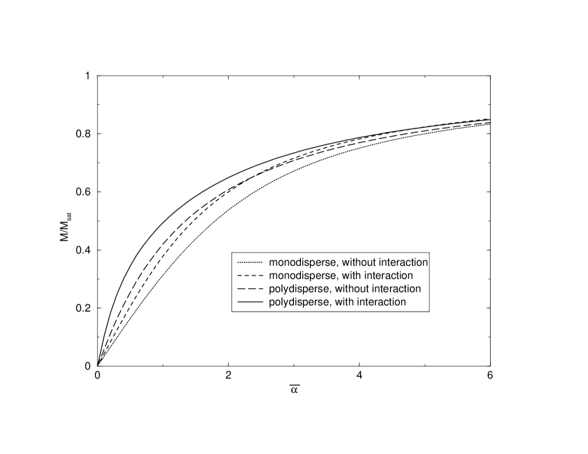
Figure 3: Equilibrium magnetization of a polydisperse ferrofluid ($\left<D_{\text{mag}}^{3}\right>_{P}^{1/3}$ = 10 nm, $\sigma=0.25$, $\mu=(D_{\text{mag}}/\overline{D})^{3}$) and a comparable monodisperse ferrofluid, both with and without taking into account the particle interaction. See text for further details.

For the monodisperse system, the magnetization contribution in $O(\overline{\phi}^{2}\overline{\epsilon}^{2})$ was calculated in Sec. V and appendix B of paper I. The cluster integrals needed in that order are shown in Fig. 3 of paper I. Some of them vanish for the same reason as the contribution $A_{1}$ in $O(\overline{\phi}\overline{\epsilon})$: They involve the averaging of a dipolar field over a spherical surface. Most of the remaining integrals cancel when the free energy $F=-kT\ln Z$ is calculated. Up to $O(\overline{\epsilon}^{2})$ we can write the remaining term in Eq. (20) as

$$\left<f_{ij}f_{ik}f_{jk}\right>_{0} = \left<f^{(0)}_{ij}f^{(0)}_{ik}f^{(0)}_{jk}\right>_{0}+3\left<f^{(2)}_{ij}f^{(0)}_{ik}f^{(0)}_{jk}\right>_{0}$$ (40)

$$+3\left<f^{(1)}_{ij}f^{(1)}_{ik}f^{(0)}_{jk}\right>_{0}\;\;.$$

These three terms correspond to the graphs E, G and H in paper I. The first one is an $O(\overline{\phi}^{2}\overline{\epsilon}^{0})$–term that does not contribute to the magnetization.

III.4.1 Graph G

Here we give an outline of the polydisperse generalization of the calculation pertaining to graph G (appendix B.7 of paper I). The quantity $Z_{G}$ calculated in paper I, is given by the sum

$$Z_{G}=Z_{0}\frac{1}{2}{\sum}^{\prime}\left<f^{(2)}_{ij}f^{(0)}_{jk}f^{(0)}_{ki}\right>_{0}$$ (41)

over distinct particles $i,j,k$. For calculating $\left<f^{(2)}_{ij}f^{(0)}_{jk}f^{(0)}_{ki}\right>_{0}$ one starts with the trivial integrations: the degrees of freedom of all particles except $i$, $j$, and $k$, the position of the center of mass of the three remaining particles, and the orientation of ${\bf m}_{k}$, since particle $k$ is not involved in dipolar interactions in this cluster. Then, for a fixed distance $r_{ij}$ the integrations over $\omega_{ij}$, $\Omega_{i}$, and $\Omega_{j}$, defined as in Sec. III.3 are carried out. This introduces the function $G_{2}^{P}$ into the result:

$$\left<f_{ij}^{(2)}f_{ik}^{(0)}f_{jk}^{(0)}\right>_{0}=\frac{36}{\pi N^{2}}(\mu_{i}\mu_{j})^{2}\overline{\phi}^{2}\overline{\epsilon}^{2}G^{P}_{2}(\alpha_{si},\alpha_{sj})$$

$$\qquad\times\int r_{ij}^{-4}e^{-v_{ij}^{HC}}f_{ik}^{(0)}f_{jk}^{(0)}\;dr_{ij}d{\bf r}_{ik}\;\;.$$ (42)

The integral over ${\bf r}_{ik}$ can be described by the following geometrical considerations: The volume of possible positions of particle $k$ has to be found, such that this particle overlaps with both, particle $i$ (i. e. $r_{ik}<D_{ik}$) and $j$ ($r_{jk}<D_{jk}$). Otherwise the integral would vanish because of the factor $f_{ik}^{(0)}f_{jk}^{(0)}$. This is only possible, if $r_{ij}<D_{ik}+D_{jk}$.

In a final step the integration over $r_{ij}$ between $D_{ij}$ and $D_{ik}+D_{jk}$ is carried out. The final result is

$$\left<f_{ij}^{(2)}f_{ik}^{(0)}f_{jk}^{(0)}\right>_{0} = \frac{3}{N^{2}}(\mu_{i}\mu_{j})^{2}\overline{\phi}^{2}\overline{\epsilon}^{2}G^{P}_{n}(\alpha_{si},\alpha_{sj})$$ (43)

$$\times f^{G}(\Delta_{ij},\Delta_{ik},\Delta_{jk})\;\;.$$

The function $f^{G}(\Delta_{ij},\Delta_{ik},\Delta_{jk})$ is given in the appendix. The contribution to the free energy is according to Eq. (20) and Eq. (40) given by

$$-kT\frac{1}{6}{\sum}^{\prime}3\left<f^{(2)}_{ij}f^{(0)}_{jk}f^{(0)}_{ki}\right>_{0}$$

$$\qquad=-NkT\overline{\phi}^{2}\overline{\epsilon}^{2}\frac{1+6\ln 2}{4}\widetilde{G}_{\text{poly},2}(\overline{\alpha}_{s})\;\;.$$ (44)

The function

$$\widetilde{G}_{\text{poly},2}(\overline{\alpha}_{s})=\frac{6}{1+6\ln 2}$$ (45)

$$\qquad\times\frac{1}{N^{3}}{\sum}^{\prime}(\mu_{i}\mu_{j})^{2}G^{P}_{n}(\alpha_{si},\alpha_{sj})f^{G}(\Delta_{ij},\Delta_{ik},\Delta_{jk})\;\;,$$

was defined in such a way, that it reduces to $G_{2}(\alpha_{s})$ in the monodisperse case. Finally introducing the diameter distribution function $P(\Delta)$ requires the replacement

$$\frac{1}{N^{3}}{\sum}^{\prime}\rightarrow\int P(\Delta_{i})\,d\Delta_{i}P(\Delta_{j})\,d\Delta_{j}P(\Delta_{k})\,d\Delta_{k}$$ (46)

in eqs. (44,45).

III.4.2 Graph H

The integrations to calculate $\left<f^{(1)}_{ij}f^{(1)}_{jk}f^{(0)}_{ki}\right>_{0}$ are performed as follows (compare to appendix B.8 in paper I): After doing the trivial integrations (concerning the possible configurations of the particles except $i$, $j$, and $k$, and the center of mass of the cluster), the possible orientations of the cluster are integrated out. Then, the integrations over the orientations of ${\bf m}_{i}$, ${\bf m}_{j}$, and ${\bf m}_{k}$ are performed. One arrives at

$$\left<f_{ij}^{(1)}f_{ik}^{(1)}f_{jk}^{(0)}\right>_{0}=\mu_{i}^{2}\mu_{j}\mu_{k}\overline{\epsilon}^{2}\frac{4\pi^{2}}{15V^{2}}K^{P}(\alpha_{si},\alpha_{sj},\alpha_{sk})$$

$$\qquad\times\int\frac{\overline{D}^{6}}{r_{ij}r_{ik}}\left(3\cos^{2}\vartheta_{jk}-1\right)e^{-v_{ij}^{HC}}e^{-v_{ik}^{HC}}f_{jk}^{(0)}$$

$$\qquad\qquad\times\text{d}r_{ij}\text{d}r_{ik}\sin\vartheta_{jk}\text{d}\vartheta_{jk}\;\;.\qquad\qquad$$ (47)

This is up to a factor $N^{2}Z_{0}/2$ a polydisperse generalization of Eq. (B21) of paper I. The remaining integrations concern the distances $r_{ij}$ and $r_{ik}$, and the angle $\vartheta_{jk}$ between ${\bf r}_{ij}$ and ${\bf r}_{ik}$. The function $K^{P}$ is defined by

$$K^{P}(\alpha_{si},\alpha_{sj},\alpha_{sk})=\frac{3}{8}\frac{(4\pi V)^{3}}{z_{i}z_{j}z_{k}}$$

$$\qquad\times\int_{-1}^{1}\int_{-1}^{1}\int_{-1}^{1}e^{\left(\alpha_{si}u_{i}+\alpha_{sj}u_{j}+\alpha_{sk}u_{k}\right)}$$ (48)

$$\qquad\qquad\times\left(3+u^{2}_{i}\right)u_{j}u_{k}\,\text{d}u_{i}\text{d}u_{j}\text{d}u_{k}$$

[compare to Eq. (B22) of paper I]. An expression for the monodisperse counterpart $K(\alpha_{s})$ was given in appendix A of paper I. Here we express $K^{P}$ via Langevin functions:

$$K^{P}(\alpha_{si},\alpha_{sj},\alpha_{sk})=$$

$$\qquad 3{\cal L}(\alpha_{sj}){\cal L}(\alpha_{sk})\left[3+{\cal L}^{\prime}(\alpha_{si})+{\cal L}(\alpha_{si})^{2}\right]\;\;.$$ (49)

Note that $r_{ij}>D_{ij}$ and $r_{ik}>D_{ik}$ is required, otherwise the integral (47) vanishes. The requirement that particles $j$ and $k$ have to overlap imposes the additional restrictions $|r_{ij}-r_{ik}|<D_{jk}$ and

$$\vartheta_{jk}<\vartheta^{\text{max}}_{jk}=\arccos\frac{r_{ij}^{2}+r_{ik}^{2}-D_{jk}^{2}}{2r_{ij}r_{ik}}\;\;.$$ (50)

After performing the remaining integrations within these limits the result is

$$\left<f_{ij}^{(1)}f_{ik}^{(1)}f_{jk}^{(0)}\right>_{0}=\mu_{i}^{2}\mu_{j}\mu_{k}\overline{\phi}^{2}\overline{\epsilon}^{2}\frac{48}{5N^{2}}$$

$$\qquad\times K^{P}(\alpha_{si},\alpha_{sj},\alpha_{sk})f^{K}(\Delta_{ij},\Delta_{ik},\Delta_{jk})\;\;.$$ (51)

The function $f^{K}(\Delta_{ij},\Delta_{ik},\Delta_{jk})$ is given in the appendix. The contribution to the free energy is

$$-kT\frac{1}{6}{\sum}^{\prime}3\left<f^{(1)}_{ij}f^{(1)}_{jk}f^{(0)}_{ki}\right>_{0}=NkT\overline{\phi}^{2}\overline{\epsilon}^{2}K_{\text{poly}}(\overline{\alpha}_{s})\;\;,$$ (52)

with

$$K_{\text{poly}}(\overline{\alpha}_{s})=-\frac{24}{5}\frac{1}{N^{3}}{\sum}^{\prime}\mu_{i}^{2}\mu_{j}\mu_{k}$$ (53)

$$\qquad\times K^{P}(\alpha_{si},\alpha_{sj},\alpha_{sk})f^{K}(\Delta_{ij},\Delta_{ik},\Delta_{jk})\;\;.$$

III.4.3 The magnetization contribution

Inserting Eq. (44) and Eq. (52) in Eq. (20) and calculating the equilibrium magnetization results in an additional $O(\overline{\phi}^{2}\overline{\epsilon}^{2})$–term in Eq. (37):

$$\frac{N\overline{m}}{\mu_{0}V}\overline{\phi}^{2}\overline{\epsilon}^{2}\left[\frac{1+6\ln 2}{4}\widetilde{G}_{\text{poly},2}^{\prime}(\overline{\alpha}_{s})-K_{\text{poly}}^{\prime}(\overline{\alpha}_{s})\right]\;\;.$$ (54)

The expansion and iteration procedure to switch from $\overline{\alpha}_{s}$ to $\overline{\alpha}$ is identical to the monodisperse case in paper I. The full expression for the magnetization containing all calculated terms reads

$$M = \frac{N\overline{m}}{\mu_{0}V}\Biggl{[}{\cal L}_{\text{poly}}(\overline{\alpha})+8\overline{\phi}\overline{\epsilon}{\cal L}_{\text{poly}}(\overline{\alpha}){\cal L}_{\text{poly}}^{\prime}(\overline{\alpha})$$

$$\qquad+\sum_{n=2}^{\infty}\overline{\phi}\overline{\epsilon}^{n}G_{\text{poly},n}^{\prime}(\overline{\alpha})$$

$$\qquad+64\overline{\phi}^{2}\overline{\epsilon}^{2}{\cal L}_{\text{poly}}(\overline{\alpha}){\cal L}_{\text{poly}}^{\prime}(\overline{\alpha})^{2}$$

$$\qquad+32\overline{\phi}^{2}\overline{\epsilon}^{2}{\cal L}_{\text{poly}}(\overline{\alpha})^{2}{\cal L}^{\prime\prime}_{\text{poly}}(\overline{\alpha})$$

$$\qquad+\overline{\phi}^{2}\overline{\epsilon}^{2}\frac{1+6\ln 2}{4}\widetilde{G}_{\text{poly},2}^{\prime}(\overline{\alpha})-\overline{\phi}^{2}\overline{\epsilon}^{2}K_{\text{poly}}^{\prime}(\overline{\alpha})\Biggr{]}\;\;.$$

IV Selected results for the magnetization

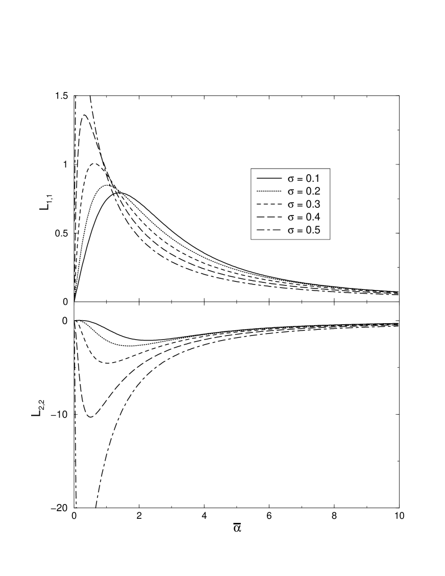
Figure 1: The contributions $L_{1,1}$ and $L_{2,2}$ as functions of $\overline{\alpha}$ for lognormal distributions with different widths $\sigma$. Here $\left<\Delta^{3}\right>_{P}=1$ and $\mu(\Delta)=\Delta^{3}$.

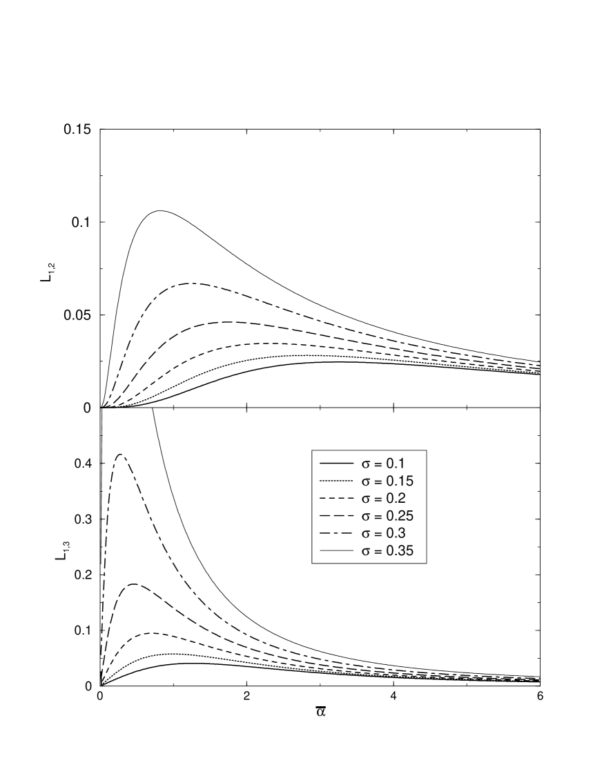
Figure 2: The contributions $L_{1,2}$ and $L_{1,3}$ as a function of $\overline{\alpha}$ for lognormal distributions with different widths $\sigma$. $\Delta$ and $\mu(\Delta)$ as in Fig. 1.

The figures 1 and 2 showing separate contributions to $M(\overline{\alpha})$ in polydisperse systems were obtained by using lognormal distributions

$$P(D)=\frac{1}{\sqrt{2\pi}\sigma D_{0}}e^{-\sigma^{2}/2}e^{-\ln^{2}(D/D_{0})/(2\sigma^{2})}$$ (56)

for the particle diameters as a representative and often used example for size distibutions of model polydisperse systems. Using similar distributions like, e. g.,  Gamma distributions, however, would not qualitatively modify the results. In Sec. V we use also an experimentally determined size distribution. Here, the quantity $\overline{D}$ was taken to be defined via the mean volume (17), i.e., $\overline{D}^{3}=\left<D^{3}\right>_{P}=D_{0}^{3}e^{15\sigma^{2}/2}$ so that $\overline{\phi}$ is the volume fraction $\phi$. The magnetic moments of the particles were taken to scale with their volumes, $m\sim D^{3}$, allowing to set $\mu(\Delta)=\Delta^{3}$ such that $\overline{m}=\left<m\right>_{P}$.

Figures 1 and 2 show the contributions

$$L_{1,1}(\overline{\alpha}) = 8{\cal L}_{\text{poly}}(\overline{\alpha}){\cal L}_{\text{poly}}^{\prime}(\overline{\alpha})\;\;,$$ (57)

$$L_{2,2}(\overline{\alpha}) = 64{\cal L}_{\text{poly}}(\overline{\alpha}){\cal L}_{\text{poly}}^{\prime}(\overline{\alpha})^{2}$$

$$+32{\cal L}_{\text{poly}}(\overline{\alpha})^{2}{\cal L}^{\prime\prime}_{\text{poly}}(\overline{\alpha})$$

$$+\frac{1+6\ln 2}{4}\widetilde{G}_{\text{poly},2}^{\prime}(\overline{\alpha})-K_{\text{poly}}^{\prime}(\overline{\alpha})\;\;,$$

$$L_{1,2}(\overline{\alpha}) = G_{\text{poly},2}^{\prime}(\overline{\alpha})\;\;,$$ (59)

$$L_{1,3}(\overline{\alpha}) = G_{\text{poly},3}^{\prime}(\overline{\alpha})$$ (60)

to $M(\overline{\alpha})$ (III.4.3) for different values of the width $\sigma$ of the distribution (56). The contributions of higher-order terms increase with growing $\sigma$. This is so because they depend on higher moments of the distribution $P(\Delta)$ that grow with the width of the distribution, even if the third moment $\left<\Delta^{3}\right>_{P}$ is kept fixed. The shift of the maxima of the curves to the right has a similar reason: Bigger particles, that react to smaller fields get more and more important when the width of the distribution grows.

The assumption $\mu(\Delta)=\Delta^{3}$ that the magnetic moments in our ferrofluid model scale $\sim D^{3}$ with the total volume of its hard sphere constituents is somewhat too simple for particles in real ferrofluids for two reasons: First, in the common case of steric stabilization by polymers surfactants providing the repulsion the surfactant layer of about 1 – 3 nm does not contribute to the magnetic moment. Second, an outer layer of the magnetic material might be magnetically dead so that it does not contribute to the magnetic moment either. For magnetite particles a dead layer depth of $\approx$ 0.8 nm has been reported SISI87 . To account for the sum of these two effects we have introduced in our calculation for $M$ an effective magnetic diameter $D_{\text{mag}}$ via the relation $D=D_{\text{mag}}+5.6\text{ nm}$. It ascribes to every particle that has a magnetically effective core of diameter $D_{\text{mag}}$ a hard sphere with a magnetically inert layer of depth 2.8 nm. The magnetic moment of each particle was then taken to scale with is magnetically effective volume, i.e., $\mu=(D_{\text{mag}}/\overline{D})^{3}$.

The full line in Fig. 3 shows the reduced equilibrium magnetization of an interacting polydisperse ferrofluid as function of $\overline{\alpha}$. Here each particle has a total magnetic inactive layer of 2.8 nm and the diameters $D_{\text{mag}}$ of the magnetic cores are lognormally distributed with $\sigma=0.25$ and $\left<D_{\text{mag}}^{3}\right>_{P}^{1/3}$ = 10 nm. The latter is taken as the reference diameter $\overline{D}$ in the calculation. The particle density is chosen in such a way that $\overline{\phi}=0.05$. Note that here $\overline{\phi}=\phi_{\text{mag}}$, the volume fraction of the magnetically active material. The magnetic moment $\overline{m}$ for $D_{\text{mag}}=$ 10 nm is chosen such that $\overline{\epsilon}=2$. The magnetization of the core is then about 550 kA/m at room temperature which is a little bit larger than that of magnetite.

Expansion terms of order $\overline{\phi}\overline{\epsilon}^{n}$ are taken into account up to order $n$=5 for the magnetization curves in Fig. 3. Higher $O(\overline{\phi}\overline{\epsilon}^{n})$–terms have only a small effect on the magnetization. Here $\overline{\epsilon}$ is by definition of $\overline{m}$ and $\overline{D}$ a typical interaction energy divided by $kT$ for particles at a distance of $\overline{D}$ = 10 nm. But with the two additional dead layers of total size 5.6 nm in between the particles of our model ferrofluid the real typical dipolar energies at contact are smaller.

The magnetization is compared to that of a polydisperse fluid without particle–particle interaction (long dashed line), and to a monodisperse ferrofluid, both with and without taking into account the particle–particle interaction (short dashed and dotted line, respectively). The monodisperse system consists of particles with $D_{\text{mag}}=$ 10 nm with the same nonmagnetic layer thickness, bulk magnetization, and $\phi_{\text{mag}}$ as before.

One sees that taking into account polydispersity or particle interaction alone strengthens the magnetization and especially the initial susceptibility. Both effects are comparable for the given parameters. Together, they result in an even higher equilibrium magnetization.

Figure 4 shows magnetization curves for magnetite–based ferrofluids with a bulk magnetization of 480 kA/m for distributions of different widths. $D_{\text{mag}}$ is taken to be lognormally distributed with $\left<D_{\text{mag}}^{3}\right>_{P}=(8\text{ nm})^{3}$ and $\sigma=$ 0.2, 0.3, and 0.4. The volume fraction of the magnetic material is $\phi_{\text{mag}}=0.1$. The particles are again assumed to carry a nonmagnetic layer of 2.8 nm thickness.

The increase in $\sigma$ causes an increase of the initial susceptibility already in the noninteracting case (long dashed lines). Including the $O(\overline{\phi}\overline{\epsilon})$–terms (short dashed lines) has a positive effect on the magnetization. The relative increase is maximal for small $\overline{\alpha}$. The magnetization decreases again at higher $\overline{\alpha}$, if higher order terms are taken into account (solid lines). For the considered ferrofluids the $O(\overline{\phi}^{2}\overline{\epsilon}^{2})$–term that is negative for higher $\overline{\alpha}$ (see Fig. 1) is almost solely responsible for this decrease. The positive contributions from the higher $O(\overline{\phi}\overline{\epsilon}^{n})$–terms ($n\geq 2$) are again negligible, except for $\sigma=0.4$ and small $\overline{\alpha}$, where they cause a further increase of the initial susceptibility. For small $\overline{\alpha}$ the $O(\overline{\phi}^{2}\overline{\epsilon}^{2})$–term also has a positive effect, but this effect is too small to be visible. The plots show again, that the influence of higher order terms is larger for broad distributions.

V Comparison to experiments

We compared our theorerical predictions for the magnetization curves with experimental results of two different magnetite–based ferrofluids. S. Odenbach (ZARM, Bremen) provided data on the equilibrium magnetization of the ferrofluid EMC 905 produced by FerroTec. We fitted our theoretical result (III.4.3) taking into account the terms in $O(\phi\epsilon^{n})$ up to $n=5$ to the data assuming lognormally distributed $D_{\text{mag}}$ and a nonmagnetic layer of depth 2.8 nm. The bulk magnetization of magnetite was taken to be 480 kA/m. The result is shown in Fig. 5. According to the fit, the saturation magnetization of the ferrofluid is $M_{\text{sat}}=37.4$ kA/m. The parameters defining the distribution turn out to be $D_{0}=8.3$ nm and $\sigma=0.28$. There are small differences between the data and the fit curve that are in our opinion due to deviations of the real diameter distribution curve from the idealized lognormal form.

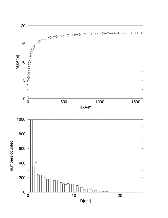
Figure 6: Top: equilibrium magnetization of the ferrofluid APG 933. Circles: experiment, solid line: the theoretical magnetization curve. Bottom: diameter distribution according to TEM measurements.

J. Embs (Universität des Saarlandes, Saarbrücken) measured the equilibrium magnetization curve of the ferrofluid APG 933 of FerroTec. In addition he determined the diameter distribution of its particles by transmission electron microscopy (TEM) which was then used in our theoretical analysis. Diameters found in TEM measurements are those of the magnetite particles. We assumed the magnetically effective diameters $D_{\text{mag}}$ to be $2\times 0.8$ nm $=1.6$ nm smaller and to be zero for particles smaller than 1.6 nm. The hard core diameters $D$ were taken to be $2\times 2$ nm $=4$ nm larger than the diameters obtained from the TEM measurements. As above, we took into account terms up to $O(\phi\epsilon^{5})$ and set the bulk magnetization of magnetite to 480 kA/m. Fig. 6 shows the TEM data and the experimental magnetization curve together with the results of our theory. Both agree very well.

VI Conclusion

In this paper we used the technique of cluster expansion to derive an approximation to the equilibrium magnetization for the system of dipolar hard spheres in a magnetic field with diameter and/or magnetic moment dispersion as a model system for a polydisperse ferrofluid. The calculation results in an expression for the magnetization $M$ in form of a twofold series expansion in the parameters $\overline{\phi}$, closely related to the volume fraction $\phi$, and $\overline{\epsilon}$, a coupling parameter measuring the strength of the dipolar interaction:

$$M=\frac{N\overline{m}}{\mu_{0}V}\sum_{m=0}^{\infty}\sum_{n=0}^{\infty}\overline{\phi}^{m}\overline{\epsilon}^{n}L_{m,n}(\overline{\alpha})\;\;.$$ (61)

$\overline{\phi}$, $\overline{\epsilon}$, and the dimensionless magnetic field $\overline{\alpha}$ are defined for some typical values $\overline{D}$ and $\overline{m}$ for the hard sphere diameters and magnetic moments respectively. $\overline{m}$ can be chosen in such a way that the prefactor $N\overline{m}/\mu_{0}V$ reduces to the saturation magnetization of the system. We gave expressions for $L_{1,n}$ ($n\leq 5$) and $L_{2,2}$. Lower orders vanish, except for $L_{0,0}$ reducing to the Langevin function in the monodisperse case. The calculated $L_{m,n}$ can be written as multiple sums over all particles whose addends are analytical expressions.

The influence of particle–particle interaction grows with increasing width of the considered diameter distribution. Taking into account only the $L_{1,1}$–term results in an increase of the magnetization relative to the non interacting system, whereas the $L_{2,2}$–term leads again to somewhat smaller values at higher $\overline{\alpha}$. Only at very small $\overline{\alpha}$ its contribution is positive. The $L_{1,n}$–terms have little effect for realistic, magnetite–based ferrofluids, except for broad distributions, where they increase the initial magnetization.

Appendix A The functions $G_{n}^{P},f^{G},f^{K}$

The functions $G_{n}^{P}(x_{1},x_{2})$ are symmetric in their arguments and have the form

$$G_{n}^{P}(x_{1},x_{2})=G^{P(0)}_{n}(1/x_{1},1/x_{2})$$

$$\qquad+\coth(x_{1})G^{P(1)}_{n}(1/x_{1},1/x_{2})$$ (62)

$$\qquad+\coth(x_{2})G^{P(1)}_{n}(1/x_{2},1/x_{1})\qquad$$

$$\qquad+\coth(x_{1})\coth(x_{2})G^{P(2)}_{n}(1/x_{1},1/x_{2})\;\;.$$

The $G^{P(i)}_{n}$ are polynomials and read for $n\leq 5$

$$G_{2}^{P(0)}(y_{1},y_{2}) = \frac{8}{5}+\frac{4}{5}y_{1}^{2}+\frac{4}{5}y_{2}^{2}+\frac{12}{5}y_{1}^{2}y_{2}^{2}\;\;,$$

$$G_{2}^{P(1)}(y_{1},y_{2}) = -\frac{4}{5}y_{1}-\frac{12}{5}y_{1}y_{2}^{2}\;\;,$$ (63)

$$G_{2}^{P(2)}(y_{1},y_{2}) = \frac{12}{5}\;\;.$$

$$G_{3}^{P(0)}(y_{1},y_{2}) = -\frac{4}{35}y_{1}y_{2}-\frac{24}{35}y_{1}^{3}y_{2}$$

$$-\frac{24}{35}y_{1}y_{2}^{3}-\frac{12}{7}y_{1}^{3}y_{2}^{3}\;\;,$$

$$G_{3}^{P(1)}(y_{1},y_{2}) = -\frac{4}{35}y_{2}+\frac{24}{35}y_{1}^{2}y_{2}$$

$$+\frac{4}{35}y_{2}^{3}+\frac{12}{7}y_{1}^{2}y_{2}^{3}\;\;,$$

$$G_{3}^{P(2)}(y_{1},y_{2}) = \frac{16}{105}-\frac{4}{35}y_{1}^{2}-\frac{4}{35}y_{2}^{2}-\frac{12}{7}y_{1}^{2}y_{2}^{2}\;\;.$$

$$G_{4}^{P(0)}(y_{1},y_{2}) = \frac{8}{105}+\frac{4}{35}y_{1}^{2}+\frac{4}{35}y_{1}^{4}+\frac{4}{35}y_{2}^{2}$$

$$+\frac{12}{5}y_{1}^{2}y_{2}^{2}+\frac{36}{7}y_{1}^{4}y_{2}^{2}+\frac{4}{35}y_{2}^{4}$$

$$+\frac{36}{7}y_{1}^{2}y_{2}^{4}+12y_{1}^{4}y_{2}^{4}\;\;,$$

$$G_{4}^{P(1)}(y_{1},y_{2}) = -\frac{8}{105}y_{1}-\frac{4}{35}y_{1}^{3}-\frac{24}{35}y_{1}y_{2}^{2}$$

$$-\frac{36}{7}y_{1}^{3}y_{2}^{2}-\frac{8}{7}y_{1}y_{2}^{4}-12y_{1}^{3}y_{2}^{4}\;\;,$$

$$G_{4}^{P(2)}(y_{1},y_{2}) = \frac{32}{105}y_{1}y_{2}+\frac{8}{7}y_{1}^{3}y_{2}+\frac{8}{7}y_{1}y_{2}^{3}+12y_{1}^{3}y_{2}^{3}\;\;.$$

$$G_{5}^{P(0)}(y_{1},y_{2}) = \frac{12}{385}y_{1}y_{2}-\frac{104}{385}y_{1}^{3}y_{2}-\frac{60}{77}y_{1}^{5}y_{2}$$

$$-\frac{104}{385}y_{1}y_{2}^{3}-\frac{732}{77}y_{1}^{3}y_{2}^{3}-\frac{240}{11}y_{1}^{5}y_{2}^{3}$$

$$-\frac{60}{77}y_{1}y_{2}^{5}-\frac{240}{11}y_{1}^{3}y_{2}^{5}-\frac{540}{11}y_{1}^{5}y_{2}^{5}\;\;,$$

$$G_{5}^{P(1)}(y_{1},y_{2}) = -\frac{4}{231}y_{2}+\frac{4}{385}y_{1}^{2}y_{2}+\frac{60}{77}y_{1}^{4}y_{2}$$

$$+\frac{4}{385}y_{2}^{3}+\frac{172}{77}y_{1}^{2}y_{2}^{3}+\frac{240}{11}y_{1}^{4}y_{2}^{3}$$

$$+\frac{4}{77}y_{2}^{5}+\frac{60}{11}y_{1}^{2}y_{2}^{5}+\frac{540}{11}y_{1}^{4}y_{2}^{5}\;\;,$$

$$G_{5}^{P(2)}(y_{1},y_{2}) = \frac{16}{1155}+\frac{8}{1155}y_{1}^{2}-\frac{4}{77}y_{1}^{4}$$

$$+\frac{8}{1155}y_{2}^{2}-\frac{32}{77}y_{1}^{2}y_{2}^{2}-\frac{60}{11}y_{1}^{4}y_{2}^{2}$$

$$-\frac{4}{77}y_{2}^{4}-\frac{60}{11}y_{1}^{2}y_{2}^{4}-\frac{540}{11}y_{1}^{4}y_{2}^{4}\;\;.$$

It is

$$f^{G}(\Delta_{ij},\Delta_{ik},\Delta_{jk})=\ln\left(\frac{\Delta_{ik}+\Delta_{jk}}{\Delta_{ij}}\right)-\frac{3(\Delta_{ik}^{2}-\Delta_{jk}^{2})^{2}}{4\Delta_{ij}^{4}}$$

$$\qquad+\frac{8(\Delta_{ik}^{3}+\Delta_{jk}^{3})}{3\Delta^{3}_{ij}}-\frac{3(\Delta_{ik}^{2}+\Delta_{jk}^{2})}{\Delta_{ij}^{2}}$$ (67)

$$\qquad+\frac{13\Delta_{ik}^{2}+14\Delta_{ik}\Delta_{jk}+13\Delta_{jk}^{2}}{12(\Delta_{ik}+\Delta_{jk})^{2}}\;\;,$$

and

$$f^{K}(\Delta_{ij},\Delta_{ik},\Delta_{jk})=-\frac{2}{9}-\frac{5}{36}\frac{\Delta_{ij}^{6}+\Delta_{ik}^{6}+\Delta_{jk}^{6}}{\Delta_{ij}^{3}\Delta_{ik}^{3}}$$

$$\qquad-\frac{\Delta_{jk}^{2}}{4\Delta_{ij}\Delta_{ik}}-\frac{2\Delta_{jk}^{3}}{9\Delta_{ij}^{3}}-\frac{2\Delta_{jk}^{3}}{9\Delta_{ik}^{3}}$$ (68)

$$\qquad+\frac{(\Delta_{ij}^{4}+\Delta_{ik}^{4}+\Delta_{jk}^{4})(\Delta_{ij}^{2}+\Delta_{ik}^{2}+\Delta_{jk}^{2})}{8\Delta_{ij}^{3}\Delta_{ik}^{3}}\;\;.$$

When all diameters are equal, these functions reduce to

$$f^{G}(\Delta,\Delta,\Delta) = \frac{1}{6}+\ln 2\;\;,$$ (69)

$$f^{K}(\Delta,\Delta,\Delta) = -\frac{5}{24}\;\;.$$ (70)

Figure 4: Equilibrium magnetization as a function of $\overline{\alpha}$ for lognormal distributions with $\left<D_{\text{mag}}^{3}\right>_{P}^{1/3}$ = 8 nm and different widths $\sigma$. Long dashed: without particle interaction, dashed: particle interaction only in $O(\overline{\phi}\overline{\epsilon})$, solid lines: all calculated terms.

Figure 5: Equilibrium magnetization of the ferrofluid EMC 905. Dots: experiment, solid line: the theoretical magnetization curve assuming lognormally distributed $D_{\text{mag}}$, c.f. text.

References

- (1) B. Huke and M. Lücke, Phys. Rev. E 62, 6875 (2000).
- (2) R. E. Rosensweig, Ferrohydrodynamics, (Cambridge University Press, Cambrigde, U.K., 1985).
- (3) M. S. Wertheim, J. Chem. Phys. 55, 4291 (1971).
- (4) S. A. Adelman and J. M. Deutch, J. Chem. Phys. 59, 3971 (1973).
- (5) D. Isbister and R. J. Bearman, Molec. Phys. 28, 1297 (1974).
- (6) J. S. Hoye and G. Stell, J. Chem. Phys. 70, 2894 (1978).
- (7) B. Freasier, N. Hamer, and D. Isbister, Molec. Phys. 38, 1661 (1979).
- (8) J. D. Ramshaw and N. D. Hamer, J. Chem. Phys. 75, 3511 (1981).
- (9) P. T. Cummings and L. Blum, J. Chem. Phys. 85, 6158 (1986).
- (10) P. H. Fries and G. N. Patey, J. Chem. Phys. 82, 429 (1984).
- (11) P. H. Lee and B. M. Ladanyi, J. Chem. Phys. 87, 4093 (1987).
- (12) P. H. Lee and B. M. Ladanyi, J. Chem. Phys. 91, 7063 (1989).
- (13) G. Kronome, I. Szalai, and J. Liszi, J. Chem. Phys. 116, 2067 (2002).
- (14) V. I. Kalikmanov, Phys. Rev. E 59, 4085 (1999).
- (15) M. I. Shliomis, A. F. Pshenichnikov, K. I. Morozov, and I. Yu. Shurubor, J. Magn. Magn. Mater. 85, 40 (1990).
- (16) K. I. Morozov and A. V. Lebedev, J. Magn. Magn. Mater. 85, 51 (1990).
- (17) Y. A. Buyevich and A. O. Ivanov, Physica A, 190, 276 (1992).
- (18) A. F. Pshenichnikov, V. V. Mekhonoshin, and A. V. Lebedev, J. Magn. Magn. Mater. 161, 94 (1996).
- (19) A. O. Ivanov and O. B. Kuznetsova, Phys. Rev. E 64, 041405 (2001).
- (20) A. O. Cebers, Magn. Gidrodinamika 2, 42 (1982).
- (21) S. Banerjee, R. B. Griffiths, and M. Widom, J. Stat. Phys. 93, 109 (1998).
- (22) T. Sato, T. Iijima, M. Seki, and N. Inagaki: J. Magn. Magn. Mater. 65, 252 (1987).