Anomalous Heat Conduction in Quasi-One-Dimensional Gases

Abstract

From three-dimensional linearized hydrodynamic equations, it is found that the heat conductivity is proportional to $(L_{x}/(L_{y}^{2}L_{z}^{2}))^{1/3}$, where $L_{x}$, $L_{y}$ and $L_{z}$ are the lengths of the system along the $x$, $y$ and $z$ directions, and we consider the case in which $L_{x}\gg L_{y},L_{z}$. The necessary condition for such a size dependence is derived as $\phi\equiv L_{x}/(n^{1/2}L_{y}^{5/4}L_{z}^{5/4})\gg 1$, where $\phi$ is the critical condition parameter and $n$ is the number density. This size dependence of the heat conductivity has been confirmed by molecular dynamics simulation.

1 Introduction

Fourier’s law of heat conduction is a relation between the heat flux $J$ and the temperature gradient. It is given by $J=-\lambda\nabla T$, where $\lambda$ and $T$ are the heat conductivity and the temperature, respectively. Although it is widely believed that Fourier’s law is realized in many situations, recent numerical results suggest that the heat conductivity diverges in low-dimensional systems in the thermodynamic limit [1], while it is convergent in three-dimensional (3D) systems [2, 3].

Narayan and Ramaswamy [4] have found that the heat conductivity is proportional to $L^{1/3}$, with the system size $L$. They derived this result from hydrodynamic equations with thermal fluctuations in the 1D limit. This size dependence of the heat conductivity is also applicable to 1D chains [5]. These results have been confirmed in numerical simulations of the Fermi-Pasta-Ulam (FPU) chain [6], a 1D gas model [7, 8] and single-walled carbon nanotubes (SWNT) [9, 10].

In real experiments, of course, it is difficult to realize actual one- or two-dimensional systems. However, it is easy to prepare quasi-one-dimensional (Q1D) systems in which the role of one direction is dominant, and the length of the system along that direction is much greater than those along the other directions. Similarly, we can construct quasi-two-dimensional (Q2D) systems, in which two directions are dominant, the lengths of the system along those directions are much greater than those along the other direction. In this paper, we demonstrate that heat conductivities in Q1D systems diverge as $\lambda\sim(L_{x}/(L_{y}^{2}L_{z}^{2}))^{1/3}$, where $L_{x}$ is the length of the system along the $x$-direction, and we have $L_{x}\gg L_{y},L_{z}$. The necessary condition for this anomalous behavior of the heat conductivity is derived as

$$\phi\equiv\frac{L_{x}}{n^{1/2}L_{y}^{5/4}L_{z}^{5/4}}=\left(\frac{L_{x}}{\sqrt{L_{y}L_{z}}}\right)^{3/2}\frac{1}{\sqrt{N}}\gg 1,$$ (1)

where $n$ is the number density, $N$ is the number of particles in the system, and $\phi$ is the critical condition parameter. We also find that Q2D systems diverge as $\lambda\sim\sqrt{(\ln(L_{x}^{2}+L_{y}^{2}))/L_{z}}$, where $L_{x}$ and $L_{y}$ are much larger than $L_{z}$. The necessary condition to obtain this behavior is $((L_{x}^{2}+L_{y}^{2})/(nL_{z}^{5}))\ln[\sqrt{L_{x}^{2}+L_{y}^{2}}/(t_{0}c_{0})]\gg~{}1$, where $t_{0}$ is the mean free time and $c_{0}$ is the velocity of sound.

2 Derivation of the long-time tail from the hydrodynamic equations

The divergence of the transport coefficient in the thermodynamic limit originates from the long-time tail of the time correlation function, which has been confirmed by molecular dynamics (MD) simulations with hard spheres [11]. For the theoretical calculation of the long-time tail near the equilibrium state, the mode-coupling theory [12] is a powerful tool. Amongst several methods for calculating the long-time tail in the mode-coupling theory, here, we adopt the hydrodynamic approach developed by Ernst et al. [13, 14].

From the Green-Kubo formula [15, 16], the heat conductivity $\lambda$ can be calculated as

$$\lambda=\beta T^{-1}\lim_{t_{c}\to\infty}\int_{0}^{t_{c}}dt\,\,C_{\lambda}\left(t\right),$$ (2)

where $C_{\lambda}(t)$ is the time correlation function of the heat flux $J$ and $\beta=(k_{B}T)^{-1}$ with the Boltzmann constant $k_{B}$. Here, we define the $x$-component of the heat flux $J$ as

$$J\equiv\sum_{i}\left[\left(\frac{m}{2}v_{i}^{2}-\frac{5}{2}k_{B}T\right)v_{ix}+\frac{1}{2}\sum_{j\neq i}\left(\Phi(\boldsymbol{r}_{ij})v_{ix}-r_{ij,x}\frac{\partial\Phi(\boldsymbol{r}_{ij})}{\partial\boldsymbol{r}_{ij}}\cdot\boldsymbol{v}_{i}\right)\right],$$ (3)

where $v_{ix}$ is the $x$ component of the velocity of the particle $i$ in a fluid of $N$ particles, $m$ is the mass of a particle, $r_{ij,x}$ is the $x$ component of the displacement vector between particles $i$ and $j$, and $\Phi(\boldsymbol{r})$ is the intermolecular pair potential. From this point, we consider only the kinetic parts, $J_{K}$, of $J$, given by

$$J^{K}\equiv\sum_{i}\left(\frac{m}{2}v_{i}^{2}-\frac{5}{2}k_{B}T\right)v_{ix},$$ (4)

and the corresponding correlation function. Through simulations, as reported in §3, we have verified that the error introduced by ignoring the remaining terms in (3) is negligibly small.

Although the Green-Kubo formula can only be proven for infinite systems, if we apply it to finite systems, we need to introduce upper bound of the integral $t_{c}$, which represents the typical transit time, $t_{c}\sim L/c_{0}$, without taking the limit $t_{c}\to\infty$ [1].

To calculate the time correlation function, we need to solve the $d$-dimensional linearized hydrodynamic equations

$$\begin{split}\frac{\partial n(\boldsymbol{r},t)}{\partial t}=&-n\nabla\cdot\boldsymbol{u}(\boldsymbol{r},t),\\ \frac{\partial\boldsymbol{u}(\boldsymbol{r},t)}{\partial t}=&\nu\nabla^{2}\boldsymbol{u}(\boldsymbol{r},t)+\left(D_{l}-\nu\right)\nabla\left(\nabla\cdot\boldsymbol{u}(\boldsymbol{r},t)\right)\\ &-\frac{c_{0}^{2}}{\gamma}\left(\frac{\nabla n(\boldsymbol{r},t)}{n}+\alpha_{p}\nabla T(\boldsymbol{r},t)\right),\\ \frac{\partial T\left(\boldsymbol{r},t\right)}{\partial t}=&-\frac{\gamma-1}{\alpha_{p}}\nabla\cdot\boldsymbol{u}\left(\boldsymbol{r},t\right)+\gamma D_{T}\nabla^{2}T\left(\boldsymbol{r},t\right).\end{split}$$ (5)

Here, $\boldsymbol{u}$ is the velocity field and

$$\begin{split}\gamma&=\frac{c_{p}}{c_{V}},\,c_{0}=\left[\frac{\gamma}{m}\left(\frac{\partial p}{\partial n}\right)_{T}\right]^{1/2},\,\alpha_{p}=-\frac{1}{n}\left(\frac{\partial n}{\partial T}\right)_{p},\\ \nu&=\frac{\eta}{nm},\,D_{T}=\frac{\lambda}{nc_{p}},\,D_{l}=\frac{2\left(d-1\right)\eta+d\xi}{dnm},\end{split}$$ (6)

where $p$ is the pressure, and $c_{p}$ and $c_{V}$ are the heat capacities per particle at constant pressure and at constant volume, respectively. Also, $\eta$ and $\xi$ are the shear viscosity and bulk viscosity, respectively.

To solve the set of equations (5), Ernst et al. [13] use the Fourier transform with respect to space. In this paper, we use the Fourier series of the hydrodynamic variables with respect to space [17, 18], given by

$$\begin{split}\delta n\left(\boldsymbol{r},t\right)&=\frac{1}{V}\sum_{\boldsymbol{k}}e^{i\boldsymbol{q}\cdot\boldsymbol{r}}n_{\boldsymbol{q}}\left(t\right),\\ n_{\boldsymbol{q}}\left(t\right)&=\int_{V}d\boldsymbol{r}\,,e^{-i\boldsymbol{q}\cdot\boldsymbol{r}}\delta n\left(\boldsymbol{r},t\right),\end{split}$$ (7)

where $\delta n\equiv n(\boldsymbol{r},t)-n$ is the deviation from the equilibrium value, and the system is a rectangular solid $\{L_{x},L_{y},L_{z}\}$, ${q}_{i}\equiv 2\pi k_{i}/L_{i}$ ($i=x,y,z$), with integer $k_{i}$. Similarly, we introduce the Fourier components $T_{\boldsymbol{q}}(t)$ and $\boldsymbol{u}_{\boldsymbol{q}}(t)$, which are the components of $\delta T\left(\boldsymbol{r},t\right)=T\left(\boldsymbol{r},t\right)-T$ and $\boldsymbol{u}\left(\boldsymbol{r},t\right)$, respectively.

In $d$-dimensional Fourier space, Eq. (5) is converted into

$$\begin{split}\frac{\partial n_{\boldsymbol{q}}}{{\partial t}}=&-in\boldsymbol{q}\cdot{\boldsymbol{u}_{\boldsymbol{q}}},\\ \frac{\partial\boldsymbol{u}_{\boldsymbol{q}}}{{\partial t}}=&-\nu\boldsymbol{q}^{2}\boldsymbol{u}_{\boldsymbol{q}}-\left(D_{l}-\nu\right)\boldsymbol{q}\left(\boldsymbol{q}\cdot\boldsymbol{u}_{\boldsymbol{q}}\right)\\ &\,\,\,\,\,-\frac{i\boldsymbol{q}c_{0}^{2}}{\gamma}\left(\frac{n_{\boldsymbol{q}}}{n}+\alpha_{p}T_{\boldsymbol{q}}\right),\\ \frac{\partial T_{\boldsymbol{q}}}{{\partial t}}=&-\frac{\gamma-1}{\alpha_{p}}i\boldsymbol{q}\cdot\boldsymbol{u}_{\boldsymbol{q}}-\gamma D_{T}q^{2}T_{\boldsymbol{q}}.\end{split}$$ (8)

These equations can be reduced to a diagonalizable $(d+2)$-dimensional matrix equation. Here, we introduce the “hydrodynamic modes”, defined as the eigenfunctions of the form $\exp(-\omega_{q}^{j}t)$. The quantities $\omega_{q}^{j}$ in the small $q\,\,(\equiv|\boldsymbol{q}|)$ limit are calculated as the $d-1$ viscous modes [$\omega_{q}^{j}=\nu q^{2}\,\,\,(j=1,\cdots,d-1)$], the two sound modes ($\omega_{q}^{\pm}=\pm ic_{0}q+\frac{1}{2}\Gamma_{s}$), with

$$\Gamma_{s}\equiv D_{l}+\left(\gamma-1\right)D_{T},$$ (9)

and the heat mode ($\omega_{q}^{H}=D_{T}q^{2}$). The Fourier series of the hydrodynamic variables can be expressed as linear combinations of the eigenvectors of the matrix equation.

After setting the initial values used by Ernst et al. [13], $C_{\lambda}(t)$ can be calculated. When the system is sufficiently large, the most dominant part of the long-time tail of $C_{\lambda}(t)$ is the viscous-heat (VH) term, given by

$$C_{\lambda}^{VH}\left(t\right)\sim\frac{1}{V}\sum_{\boldsymbol{k}}\left(1-\hat{q}_{x}^{2}\right)\exp\left[-\left(\nu+D_{T}\right)q^{2}t\right],$$ (10)

with $\hat{q}_{i}\equiv q_{i}/q\,\,\left(i=x,y,z\right)$ and the sound-sound (SS) term,

$$C_{\lambda}^{SS}(t)\sim\frac{1}{V}\sum_{\boldsymbol{k}}\hat{q}_{x}^{2}\exp\left[-\Gamma_{s}q^{2}t\right].$$ (11)

Note that $C_{\lambda}(t)$ decays as $t^{-d/2}$ [13, 14].

In a Q1D system, however, the SS term is dominant,as seen from the following. First, let us assume that $L_{y}\simeq L_{z}$ and that $L_{x}$ is sufficiently larger than $L_{y}$ and $L_{z}$. The exponential term in the SS term in Eq. (11) is

$$\exp\left[-4\pi^{2}\Gamma_{s}\left(\frac{k_{x}^{2}}{L_{x}^{2}}+\frac{k_{y}^{2}}{L_{y}^{2}}+\frac{k_{z}^{2}}{L_{z}^{2}}\right)t\right].$$ (12)

When time is sufficiently large, i.e., $t\sim t_{c}\sim L/c_{0}$ with $L=\sqrt{L_{x}^{2}+L_{y}^{2}+L_{z}^{2}}\simeq L_{x}$, it is found that the $\{k_{y},k_{z}\}=\{0,0\}$ term is dominant in Eq. (11). Because we consider Q1D systems, we assume that the relation given by

$$\frac{\Gamma_{s}t}{L_{y}^{2}}\sim\frac{\Gamma_{s}}{c_{0}L_{y}^{2}}L_{x}\gg 1$$ (13)

is satisfied. Therefore Eq. (11) can be rewritten as

$$C_{\lambda}^{SS}\left(t\right)\sim\frac{1}{L_{y}L_{z}}\frac{1}{L_{x}}\sum_{k_{x}}\exp\left[-4\pi^{2}\Gamma_{s}\frac{k_{x}^{2}}{L_{x}^{2}}t\right].$$ (14)

If $\Gamma_{s}t/L_{x}^{2}\sim\Gamma_{s}/(c_{0}L_{x})$ is sufficiently small, this summation can be reduced to the integral form

$$\begin{split}C_{\lambda}^{SS}(t)&\sim\frac{1}{L_{y}L_{z}}\int_{0}^{\infty}dx\,\,\exp\left[-4\pi^{2}\Gamma_{s}x^{2}t\right],\\ &=\frac{1}{4\pi L_{y}L_{z}}\sqrt{\frac{\pi}{\Gamma_{s}t}},\end{split}$$ (15)

which implies that $C_{\lambda}^{SS}(t)$ decays as $t^{-1/2}$.

By contrast, the $\{k_{y},k_{z}\}=\{0,0\}$ term in the VH term of Eq. (10) cannot be dominant. Instead, the $\{k_{y},k_{z}\}=\{\pm 1,0\}$ and $\{0,\pm 1\}$ terms are dominant, and Eq. (10) can be written in the integral form

$$\begin{split}C_{\lambda}^{VH}\left(t\right)&\sim\frac{1}{L_{y}L_{z}}\int_{0}^{\infty}dx\,\,\frac{1}{1+L_{y}^{2}x^{2}}\exp\left[-4\pi^{2}(\nu+D_{T})\frac{1+L_{y}^{2}x^{2}}{L_{y}^{2}}t\right],\\ &<\frac{1}{L_{y}L_{z}}\exp\left[-4\pi^{2}\frac{\nu+D_{T}}{L_{y}^{2}}t\right]\int_{0}^{\infty}dx\,\,\exp\left[-4\pi^{2}\left(\nu+D_{T}\right)x^{2}t\right],\\ &=\frac{1}{4\pi L_{y}L_{z}}\sqrt{\frac{\pi}{(\nu+D_{T})t}}e^{-4\pi^{2}\frac{\nu+D_{T}}{L_{y}^{2}}t},\end{split}$$ (16)

which reveals that $C_{\lambda}^{VH}(t)$ decays exponentially with time. Thus, $C_{\lambda}^{VH}(t)$ decays much faster than $C_{\lambda}^{SS}(t)$. From Eq. (2), if is seen that the heat conductivity can be calculated as

$$\lambda\simeq\beta T^{-1}\int^{t_{c}}_{0}dt\,\,\left(C_{\lambda}^{SS}\left(t\right)+C_{\lambda}^{VH}\left(t\right)\right)\simeq\beta T^{-1}\int^{t_{c}}_{0}dtC_{\lambda}^{SS}(t).$$ (17)

From Eqs. (15) and (17), we need to estimate the system size dependence of $\Gamma_{s}$ in order to calculate $\lambda$. Therefore, we need to calculate the long-time tail of the shear viscosity in Q1D systems. The time correlation function of the $xy$ component of the shear stress and the corresponding viscosity are calculated as

$$\eta^{xy} = \frac{\beta}{V}\int^{t_{c}}_{0}dt\,\,C_{\eta}^{xy}(t),$$ (18)

$$C_{\eta}^{xy}(t) \equiv \mbox{$\langle J_{\eta}^{xy}(t)J_{\eta}^{xy}(0)\rangle$},$$ (19)

$$J_{\eta}^{xy}(t) \equiv \sum_{i}\left(mv_{ix}(t)v_{iy}(t)-\frac{1}{2}\sum_{j\neq i}r_{ij,x}\frac{\partial\Phi(\boldsymbol{r}_{ij})}{\partial r_{ij,y}}\right),$$ (20)

$$J_{\eta}^{K,xy} = \sum_{i}mv_{ix}(t)v_{iy}(t).$$ (21)

We consider only the kinetic parts, $J_{\eta}^{K,xy}$, of $J_{\eta}^{xy}$ and the corresponding correlation function. From the similar calculation of $C_{\lambda}(t)$, if is found that the dominant term of $C_{\eta}(t)$ for large $L_{x}$ is the viscous-viscous (VV) term from the $yz$ component of the shear stress, given by

$$\begin{split}{C_{\eta}^{yz}}^{VV}(t)\sim\sum_{\boldsymbol{k}}[\hat{q}_{x}^{2}+2\hat{q}_{y}^{2}\hat{q}_{z}^{2}]\exp[-2\nu\boldsymbol{q}^{2}t]\sim L_{x}\sqrt{\frac{1}{\nu t}}.\end{split}$$ (22)

Because the kinetic viscosity $\nu$ is proportional to $\eta$ in Eq. (6), we derive $\eta$ from Eq. (18) as

$$\eta\sim\left(\frac{L_{x}}{L_{y}^{2}L_{z}^{2}}\right)^{1/3}.$$ (23)

We assume that the bulk viscosity $\xi$ satisfies the relation

$$\eta+\xi\sim\left(\frac{L_{x}}{L_{y}^{2}L_{z}^{2}}\right)^{1/3},$$ (24)

which is realized in most normal fluids. Therefore, $\Gamma_{s}$ can be expressed as

$$\Gamma_{s}\sim C_{1}\lambda+C_{2}\left(\frac{L_{x}}{L_{y}^{2}L_{z}^{2}}\right)^{1/3},$$ (25)

where $C_{1}$ and $C_{2}$ are constants that are independent of time and the system size. Thus, from Eqs. (15), (17) and (25), we can derive the following self-consistent equation for $\lambda$:

$$C_{1}\lambda^{3}+C_{2}\left(\frac{L_{x}}{L_{y}^{2}L_{z}^{2}}\right)^{1/3}\lambda^{2}\sim\frac{L_{x}}{L_{y}^{2}L_{z}^{2}}.$$ (26)

This equation indicates that the system size dependence of $\lambda$ is given by

$$\lambda\sim\left(\frac{L_{x}}{L_{y}^{2}L_{z}^{2}}\right)^{1/3}.$$ (27)

The necessary condition for Eq. (27) to be valid is derived from Eq. (13) as

$$\phi\gg 1.$$ (28)

The heat conductivity and shear viscosity in Q2D systems can be derived correspondingly as

$$\lambda\sim\sqrt{\frac{\ln(L_{x}^{2}+L_{y}^{2})}{L_{z}}},$$ (29)

where $L_{z}\ll L_{x},L_{y}$. The necessary condition for this anomalous behavior is derived as

$$\frac{L_{x}^{2}+L_{y}^{2}}{nL_{z}^{5}}\ln\frac{\sqrt{L_{x}^{2}+L_{y}^{2}}}{t_{0}c_{0}}\gg 1.$$ (30)

3 MD simulation

In order to check the validity of Eq. (27), we have performed 3D MD simulations with hard spheres in Q1D systems [19, 20, 21, 22]. It is noted that a logarithmic system size dependence of the heat conductivity in 2D systems has been confirmed with MD simulations with hard disks [23]. It should also be noted, however, that it is difficult to distinguish logarithmic behavior from power law behavior in 2D simulations.

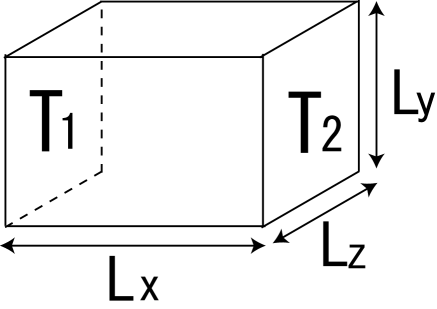
Figure 1: The system studied in the simulation. The walls perpendicular to the $y$ and $z$ directions are perfectly reflecting and those perpendicular to the $x$ direction are perfectly thermalizing. These ‘thermal’ walls are at $T_{1}$ and $T_{2}$, respectively.

In our simulations, the system is confined in a box of size ${L_{x}\times L_{y}\times L_{z}}$, as shown in Fig. 1. The walls perpendicular to the $y$ and $z$ directions are perfectly reflecting walls and the walls vertical to the $x$ direction are perfectly thermalizing walls at temperatures $T_{1}$ and $T_{2}$, respectively. At the ‘thermal’ wall of temperature $T_{w}$, a particle is reflected with a new velocity $\boldsymbol{v}$ at random. The probability distribution function for $\boldsymbol{v}$ is given by

$$\psi\left(\boldsymbol{v}\right)=\frac{2\pi|v_{x}|}{\left(2\pi k_{B}T_{w}\right)^{2}}\exp\left[-\frac{\boldsymbol{v}^{2}}{2k_{B}T_{w}}\right].$$ (31)

The MD data were taken for the systems with $\tilde{L}_{y}=\tilde{L}_{z}=0.1-3.2$ and $\tilde{L}_{x}/\tilde{L}_{y}=2-16384$, where the unit of length is the diameter of a particle and $\tilde{L}_{i}\equiv L_{i}-1$ is the range within which the center of the particle can move. For the system with $\tilde{L}_{y}=3.2$, data were taken only for $\tilde{L}_{x}/\tilde{L}_{y}=2-4096$. The packing fraction was fixed approximately to $0.055$. The ratio of the temperature difference between two thermal walls was $T_{1}/T_{2}=2$.

As the initial state, the molecules were arranged so as to realize a constant pressure under the linear profile of $T$; i.e. $nT$ is initially uniform in the system. The initial velocities of the particles were chosen from the Maxwellian distribution with $T$ varying linearly from $T_{1}$ to $T_{2}$. To obtain a stationary initial state, we simulated $6\times 10^{5}$ collisions per particle which started from the initial state. We carried out the simulation until $4\times 10^{5}$ collisions per particle were realized from the stationary initial state. The heat flux $J$ was calculated using Eq. (3). We found that in the simulation, the difference between $J$ and $J_{K}$ is less than $0.1\%$. The heat conductivity is calculated as $\lambda=-J\hat{L}_{x}/\triangle T$, where $\triangle T$ is the difference between the temperatures near the thermal walls at $T_{1}$ and $T_{2}$, respectively, and $\hat{L}_{x}$ is the distance between the points at which the temperatures are given.

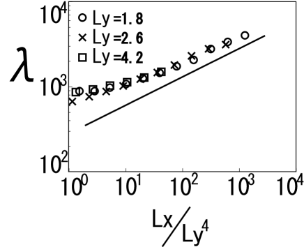
Figure 2: The size dependence of the heat conductivity in the Q1D system. The $x$-axis is $L_{x}/L_{y}^{4}$, with the unit of length being the diameter of the hard spheres. The circles, crosses and open squares indicate the heat conductivities, where $L_{y}$ is $1.8,2.6$ and $4.2$, respectively. The solid line represents a function proportional to $x^{1/3}$.

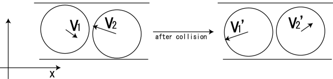
Figure 3: A collision of particle $1$ and particle $2$ for small $L_{y}$. Here, $\boldsymbol{v}_{1}$ and $\boldsymbol{v}_{2}$ are the velocities of particles $1$ and $2$ before the collision, respectively, and $\boldsymbol{v}^{\prime}_{1}$ and $\boldsymbol{v}^{\prime}_{2}$ are the velocities of particles $1$ and $2$ after the collision, respectively.

The result of the simulation is shown in Fig. 2. There, it is seen that the heat conductivity seems to obey Eq. (27) for $L_{y}\geq 1.8$, while such behavior is not observed for smaller $L_{y}$. We believe that this difference is caused by the limitation on the collision angle in the case that $\tilde{L}_{y}$ is much smaller than the diameter. For small $\tilde{L}_{y}$, as in Fig. 3, most of the collisions of the particles take place with $v^{\prime}_{1x}\simeq v_{2x}$ and $v^{\prime}_{2x}\simeq v_{1x}$, and the changes of the velocities in the other directions are small in each collision. Thus, most of the collisions cause only exchanges of the velocities of the particles in the $x$-direction, and the heat transfer behaves like that in the case of ballistic transport. In this situation, the linearized hydrodynamic equations (5) for small $L_{y}$ cannot be used. Contrastingly, for the system with $L_{y}=1.8$ and $L_{x}/(L_{y}^{2}L_{z}^{2})>10.0$, the most probable value of the exponent $\alpha$ with $L^{\alpha}$ is $0.30\pm 0.01$, which is close to $1/3$.

Although the results of our theory and simulation are consistent, we need to simulate larger systems to confirm the relation (27). There is an inconsistency in the analytical and numerical treatments. Indeed, because the linearized hydrodynamic equations (5) were adopted in the case that the system size is larger than the mean free path, but this conditions is not satisfied in our simulation, where the widths $L_{y}$ and $L_{z}$ are smaller than the mean free path by an amount on the order of $7$ diameters.

4 Discussion

We should note that Shimada et al. [2] and Ogushi et al. [3] also calculated the heat conductivity using 3D MD simulations in Q1D systems consisting of hard spheres and Lennard-Jones molecules, respectively. Their simulations suggest that the heat conductivity does not diverge in the limit $L_{x}\to\infty$. However, the system sizes in their simulations do not satisfy the necessary condition $\phi\gg 1$. In their simulations, $\phi$ is $0.03-0.3$ with $L_{y}=20.0$ and $0.3-2$ with $L_{y}=4.0$, respectively, where the unit of the length is the particle diameter. By contrast, our simulation is more extensive in the system $\phi$ is $1.8-2\times 10^{4}$ for $L_{y}=1.8$. This difference might be the cause of the qualitative difference in the behavior of the heat conductivity.

In numerical simulations of SWNT, which can be regarded as a Q1D system, $\lambda\sim L^{1/3}$ has been observed [9, 10]. In Murayama’s paper [9], it is reported that the heat conductivity behaves as $\lambda\sim L_{l}^{0.32}$, with the tube length $L_{l}$ for $(5,5)$ SWNT. However, for a wider tube diameter, $(10,10)$ SWNT, the increase of $\lambda$ is suppressed. It might be possible to understand this result in terms of the necessary condition for the anomalous behavior of the heat conductivity, $\phi\gg 1$. This behavior is also consistent with that found in our simulation. As we can see in Fig. 4, anomalous behavior of the heat conductivity, $\alpha\simeq 1/3$, with $\lambda\sim L_{x}^{\alpha}$, is observed for $L_{x}>10^{3}$, with $L_{y}=1.8$ where $\phi$ is larger than the critical value, $\phi_{c}=7.1\times 10^{2}$. By contrast, for a wider tube diameter, $L_{y}=4.2$, the increase of $\lambda$ is suppressed. From the necessary condition (28), the anomalous behavior $\alpha\simeq 1/3$ may be observed for $L_{x}>8.4\times 10^{3}$ for the wider tube diameter $L_{y}=4.2$, for which $\phi>\phi_{c}$ is satisfied. Similarly, for $(10,10)$ SWNT, anomalous behavior of the heat conductivity might be observed for a longer tube, because $\phi\gg 1$ is satisfied in that case.

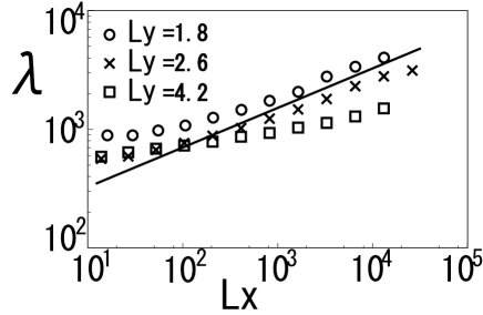
Figure 4: The size dependence of the heat conductivity in the Q1D system. The $x$-axis is $L_{x}$, with the unit of length being the diameter of the hard spheres. The circles, crosses and open squares indicate the heat conductivities, where $L_{y}$ is $1.8,2.6$ and $4.2$, respectively. The solid line represents a function proportional to $x^{1/3}$.

Recently, Shiba et al. [24] observed that the time correlation function of the heat flux is proportional to $t^{-0.98\pm 0.25}$, and the heat conductivity exhibits logarithmic divergence with the system size in three-dimensional FPU-$\beta$ lattice systems. They also measured the size dependence of the heat conductivity in Q1D FPU-$\beta$ lattices. Figure $4$ in their paper suggests that when the system is sufficiently close to a Q1D system, the heat conductivity is proportional to $L^{1/3}$.

In conclusion, we derived relation according to which the heat conductivity is proportional to $(L_{x}/L_{y}^{2}L_{z}^{2})^{1/3}$ in Q1D systems and $\sqrt{(\ln{(L_{x}^{2}+L_{z}^{2})})/L_{y}}$ in Q2D systems, and the necessary conditions $L_{x}^{4}/(n^{2}L_{y}^{5}L_{z}^{5})\gg 1$ and                           $((L_{x}^{2}+L_{y}^{2})/(nL_{z}^{5}))\ln[\sqrt{L_{x}^{2}+L_{y}^{2}}/(t_{0}c_{0})]\gg 1$, respectively, for the anomalous behavior of the heat conductivity from linearized hydrodynamic equations. This behavior in Q1D systems has been confirmed through comparison with MD simulations.

References

• [1] S. Lepri, R. Livi and A. Politi, \PRP377,2003,1.
• [2] T. Shimada, T. Murakami, S. Yukawa, K. Saito and N. Ito, \JPSJ69,2000,3150.
• [3] F. Ogushi, S, Yukawa and N. Ito, \JPSJ74,2005,827.
• [4] O. Narayan and O. Ramaswamy, \PRL89,2002,200601.
• [5] T. Mai and O. Narayan, \PRE73,2006,061202.
• [6] J.-S. Wang and B. Li, \PRL92,2004,074302.
• [7] P. Grassberger, W. Nadler and L. Yang, \PRL89,2002,180601.
• [8] P. Cipriano, S. Denisov and A. Politi, \PRL94,2005,244301.
• [9] S. Murayama, \JLPhysica B,323,2002,193.
• [10] G. Zhang and B. Li, \JLJ. Chem. Phys.,123,2005,014705.
• [11] B. J. Alder and T. E. Wainwright, \PRA1,1970,18.
• [12] Y. Pomeau and P. Resibois, \PRP19,1975,64.
• [13] M. H. Ernst, E. H. Hauge and J. M. J. van Leeuwen, \PRA4,1971,2055.
• [14] M. H. Ernst, E. H. Hauge and J. M. J. van Leeuwen, \JLJ. Stat. Phys.,15,1976,7.
• [15] R. Kubo, \JPSJ12,1957,570.
• [16] B. Zwanzig, \JLAnnu. Rev. Phys. Chem.,16,1965,67.
• [17] T. Keyes and B. Ladanyi, \JLJ. Chem. Phys.,62,1975,4787.
• [18] J. J. Erpenbeck and W. W. Wood, \PRA26,1982,1648.
• [19] D. C. Rapaport, \JLJ. Comput. Phys.,34,1980,184.
• [20] M. Marín , D. Risso and P. Cordero, \JLJ. Comput. Phys.,109,1993,306.
• [21] M. Marín and P. Cordero, \JLComput. Phys. Commu.,92,1995,214.
• [22] M. Isobe, \JLInt. J. Mod. Phys. C, 10,1999,1281.
• [23] T. Murakami, T. Shimada, S. Yukawa and N. Ito, \JPSJ72,2003,1049.
• [24] H. Shiba, S. Yukawa and N. Ito, \JPSJ75,2006,103001.