Application of the Gillespie algorithm to a granular intruder particle

Abstract

We show how the Gillespie algorithm, originally developed to describe coupled chemical reactions, can be used to perform numerical simulations of a granular intruder particle colliding with thermalized bath particles. The algorithm generates a sequence of collision “events” separated by variable time intervals. As input, it requires the position-dependent flux of bath particles at each point on the surface of the intruder particle. We validate the method by applying it to a one-dimensional system for which the exact solution of the homogeneous Boltzmann equation is known and investigate the case where the bath particle velocity distribution has algebraic tails. We also present an application to a granular needle in bath of point particles where we demonstrate the presence of correlations between the translational and rotational degrees of freedom of the intruder particle. The relationship between the Gillespie algorithm and the commonly used Direct Simulation Monte Carlo (DSMC) method is also discussed.

1 Introduction

Kinetic theories of granular systems are usually constructed starting from the Boltzmann equation or one of its variantsGG01 ; PB03 . Rarely, it is possible to obtain an exact, analytic solution of the Boltzmann equationPTV06 . More typically, however, approximations are required. It is then highly desirable to assess the quality of the theoretical prediction by comparing it with accurate numerical solutions of the Boltzmann equation. It is the purpose of this paper to show that, besides the celebrated Direct Simulation Monte Carlo (DSMC) introduced by BirdB94 , there exists an alternative method, originally proposed by GillespieG76 ; G77 to study coupled chemical reactions.

One class of system that is amenable to a Boltzmann approach and that has received considerable attention in recent years consists of a single intruder (or tracer) particle in a bath of thermalized particlesDB05 ; BRM05 ; MP99 ; VT04 ; GTV05 ; PVTW06 , showing in particular the absence of equipartition. This phenomena has been observed experimentally in two-dimensionalFM02 and three-dimensionalWP02 granular gases. The intruder-bath particle collisions are dissipative, while the bath particles have an ideal gas structure and a specified velocity distribution characterized by a fixed temperature. Since Gaussian velocity statistics are quite rare, it is important that numerical and theoretical approaches be able to treat a general distribution.

We begin by outlining the Gillespie algorithm and how it can be used to obtain a numerical solution of the Boltzmann equation. We then illustrate the application of the algorithm with two examples. The first is a one-dimensional system consisting of an intruder particle in a bath of thermalized point particles. If the bath particles have a Gaussian velocity distribution one recovers the exact Gaussian intruder velocity distribution function MP99 with a granular temperature that is smaller than the bath temperature. In addition when we impose a power-law velocity distribution on the bath particles, we find the same form for the intruder particle distribution.

The second system is two-dimensional and consists of a needle intruder in a bath of point particles. It is known that equipartition does not hold between different degrees of freedom of the needleVT04 . Here we use the Gillespie algorithm to obtain a new physical result, namely the presence of correlations between the translational and rotational degree of freedom of the needle.

2 Algorithm

The model consists of a single intruder particle that undergoes a series of collisions with the surrounding bath particles. Let $P(t)$ denote the probability that no event (collision) has occurred in the interval $(0,t)$. Then

$$P(t+\Delta t)=P(t)(1-\phi(t)\Delta t+O(\Delta t^{2}))$$ (1)

where $\phi(t)$ is the event rate in general and the collision rate in this application. Expanding the lhs to first order in $\Delta t$ and taking the limit $\Delta t\to 0$ leads to

$$\frac{d\ln P(t)}{dt}=-\phi(t)$$ (2)

Integrating and using the boundary condition that $P(0)=1$ gives

$$P(t)=\exp\bigl{[}-\int_{0}^{t}\phi(t^{\prime})dt^{\prime}\bigr{]}$$ (3)

If $\phi(t)$ is constant between collisions this expression takes the simple form:

$$P(t)=\exp(-\phi t)$$ (4)

At the end of the waiting time an event (collision) occurs that alters the value of $\phi$ or the way that $\phi$ evolves with time. We now consider two specific applications. In the first, the flux of colliding particles is constant between collisions and the simpler form, Eq 4 may be used. Our second example, an anisotropic object that rotates between collisions, requires the use of the more general form, Eq 3.

3 Applications

3.1 One-dimensional system

Consider first a one-dimensional system consisting of an intruder particle of mass $M$ moving in a bath of thermalized point particles each of mass $m$. The dynamics of the intruder is described by the Boltzmann equation.

The velocity distribution of the bath particles is denoted by $f(v,a)$, where $a$ is related to the bath temperature, $T_{B}$.

The flux of particles that collide with the right hand side of the intruder particle moving with a velocity $v_{1}$ is:

$$\phi_{+}(v_{1}) = \rho\int_{-\infty}^{v_{1}}(v_{1}-v)f(v,a)dv,$$ (5)

where $\rho$ is the number density of the bath particles. Similarly the flux on the left hand side is:

$$\phi_{-}(v_{1}) = \rho\int_{v_{1}}^{\infty}(v-v_{1})f(v,a)dv$$ (6)

and the total collision rate is

$$\phi(v_{1}) = \phi_{+}(v_{1})+\phi_{-}(v_{1})$$ (7)

Let $F(v_{1},t)$ denote the time-dependent distribution function of tracer particle velocity. Then this evolves according to

$$\frac{\partial F(v_{1},t)}{\partial t}=-\phi(v_{1})F(v_{1},t)+\int_{-\infty}^{\infty}\psi(v\to v_{1})F(v,t)dv$$ (8)

which is equivalent to the homogeneous Boltzmann equationPTV06 . The first term on the rhs is a loss term corresponding to the probability that a tracer particle with velocity $v_{1}$ undergoes a collision (necessarily to a different velocity) per unit time. The second, or gain, term contains the function $\psi(v\to v_{1})$ that is the rate that tracer particles moving with velocity $v$ are transformed (by collisions with the bath particles) to those moving with velocity $v_{1}$. For collisions with the rhs of the intruder particle the explicit expression is

$$\psi_{+}(v\to v_{1})=\rho\left(\frac{1+M}{1+\alpha}\right)^{2}(v-v_{1})f(v+\frac{1+M}{1+\alpha}(v_{1}-v),a),$$ (9)

with $v_{1}<v$. A similar expression applies for collisions on the left hand side of the intruder particle. We note that a representation of the Boltzmann equation similar to Eq 8 was employed by Puglisi et al. PVTW06 .

The Gillespie algorithm provides an numerical solution of Eq 8, including the transient case when the derivative is not equal to zero.

If the intruder particle moves with a constant velocity the flux is itself (on average) constant. A waiting time consistent with Eq 3 is then generated:

$$\Delta t=-\ln(\xi_{1})/\phi(v_{1}),$$ (10)

where $0<\xi_{1}<1$ is a uniform random number.

Given a collision at time $t$, the probability that the collision occurs on the right is given by

$$p(+|t)=\phi_{+}(v_{1})/\phi(v_{1}).$$ (11)

This is sampled by generating a second uniform random number $0<\xi_{2}<1$. If $\xi_{2}<p(+|t)$ the collision is on the right hand side: otherwise it takes place on the left hand side.

Having chosen the side, it is then necessary to sample the velocity of the bath particle that collides with this side. The probability distribution function of the colliding particle’s velocity depends on the collision side:

$$g_{+}(v,v_{1})=\left\{\begin{array}[]{ll}(v_{1}-v)f(v,a)/\phi_{+}(v_{1})&\mbox{if $v\leq v_{1}$}\\ 0&\mbox{otherwise}\end{array}\right.$$ (14)

$$g_{-}(v,v_{1})=\left\{\begin{array}[]{ll}(v-v_{1})f(v,a)/\phi_{-}(v_{1})&\mbox{if $v\geq v_{1}$}\\ 0&\mbox{otherwise}\end{array}\right.$$ (17)

The results presented so far apply to any bath velocity distribution - and the behavior depends strongly on the exact form PVTW06 . For a Gaussian

$$f(v,a)=\sqrt{\frac{a}{\pi}}\exp(-av^{2}),\;\;-\infty<v<\infty$$ (18)

where $a=m/(2k_{B}T_{B})$. The collision fluxes on each side of the tracer particle are

$$\phi_{\pm}(v_{1})=\frac{\rho}{2}(\pm v_{1}+\frac{1}{\sqrt{\pi a}}\exp(-av_{1}^{2})+v_{1}{\rm erf}(v_{1}\sqrt{a})),$$ (19)

and the total collision rate is

$$\phi(v_{1})=\rho(\frac{1}{\sqrt{\pi a}}\exp(-av_{1}^{2})+v_{1}{\rm erf}(v_{1}\sqrt{a})).$$ (20)

This function is shown in Figure 1.

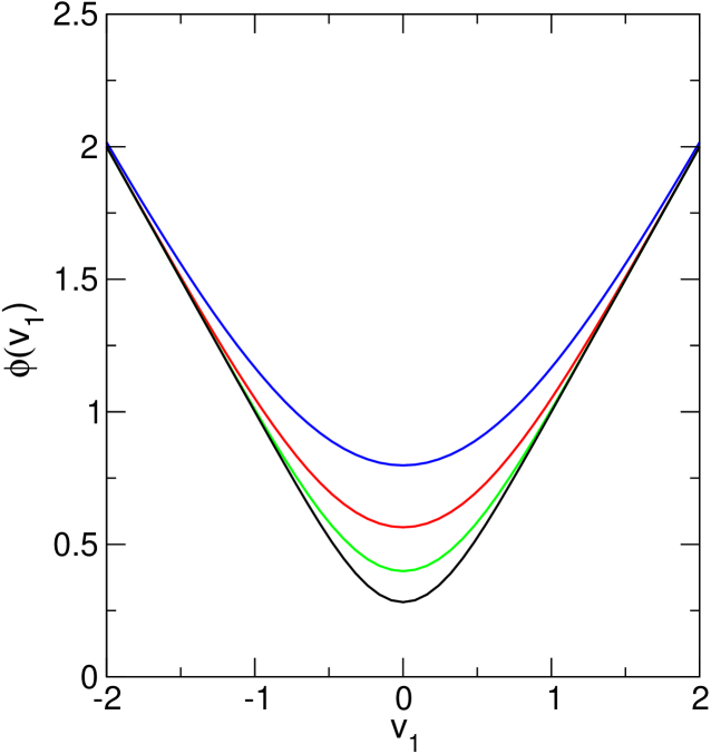
Figure 1: Flux, or collision rate, on both sides of a surface moving in a bath of particles with a Gaussian velocity distribution at a velocity $v_{1}$. $a=0.5,1,2,4$ top-to-bottom.

The velocity distribution of the colliding particles, Eq 14, in the case of a bath particle Gaussian velocity distribution is plotted in Fig 2 for several values of the intruder particle velocity. Sampling of this distribution is accomplished with an acceptance-rejection method in which the sampling region is adapted to the velocity of the intruder. A rare, but possible, case is to select a collision on the right hand side when the surface is moving rapidly to the left. The distribution of colliding particles is sharply peaked at $v_{1}$ and it is necessary to take the range of $v$ from $v_{1}-2$ to $v_{1}$. If the surface is moving to the right, the distribution of colliding particle’s velocity is more symmetric and one can sample $v$ in the range $-3\leq v\leq 3$.

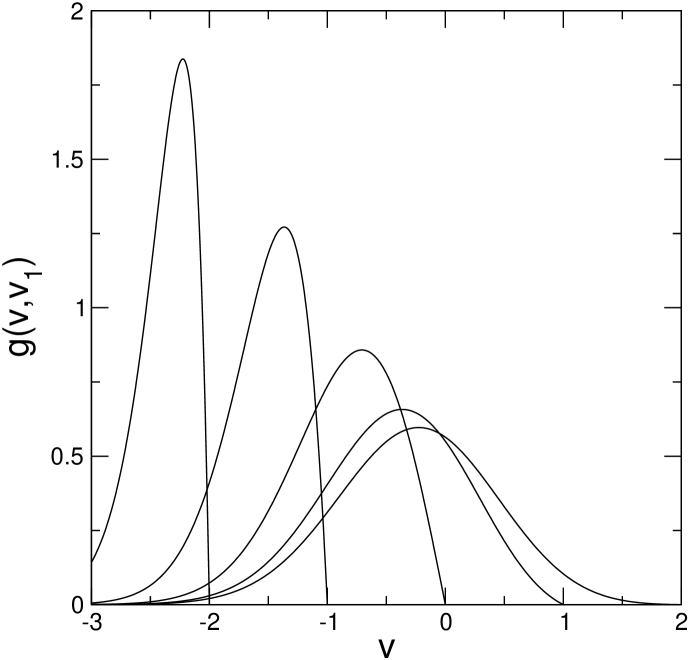
Figure 2: Probability distribution of particles that collide with the right hand side of a surface moving with a velocity $v_{1}=-2,-1,0,1,2$, left to right. The bath particles have a Gaussian velocity distribution

Finally, when the intruder particle moving with a velocity $v_{1}$ collides with a bath particle of velocity $v$ the velocity of the former changes instantaneously to

$$v_{1}^{\prime}=v_{1}+\frac{1+\alpha}{1+M}(v-v_{1}),$$ (21)

where $0<\alpha\leq 1$ is the coefficient of restitution and we have taken $m=1$ for convenience.

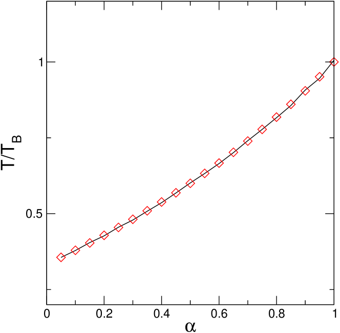
Figure 3: Ratio of the intruder granular temperature to the bath temperature. Symbols show the simulation results and the solid curve shows the theoretical prediction of Martin and Piasecki, Eq 22. Results are for $M=m$ and $n_{\rm col}=500000$

The complete algorithm describing one iteration can now be summarized using pseudocode:

• Generate a waiting time using Eq 10.

• $t\to t+\Delta t$
  while $(t_{\rm out}<t)$
  $\{t_{\rm out}\leftarrow t_{\rm out}+\delta t$
  accumulate averages$\}$

• Choose the collision side using Eq 11.

• The velocity of the colliding bath particle $v$ is sampled from the distribution given by Eq 14 or Eq 17.

• The post-collisional velocity of the intruder particle is determined from Eq 21.

Although the time increment between events is variable, averages (mean square velocities and velocity distributions) must be computed at equal time intervals. In step 2, $t$ denotes the total elapsed time and $\delta t$ is the constant time interval between the accumulation of quantities to be averaged. A convenient choice for $\delta t$ is the average collision time.

Martin and Piasecki MP99 obtained an analytic solution of the homogeneous stationary Boltzmann equation and showed that the velocity distribution of the intruder particle in the steady state is Gaussian and characterized by a temperature, $T$, that is different from the bath temperature $T_{B}$. Specifically, the two are related by:

$$\frac{T}{T_{B}}=\frac{1+\alpha}{2+(1-\alpha)/M},$$ (22)

so that for $\alpha<1$, $T<T_{B}$. Figure 3 shows an excellent agreement of the simulation with this exact result.

Since the existence of solutions of the Boltzmann equation with power-law tails has been shown recently BMM05 ; BM05 , it is interesting to investigate this phenomenon in the intruder particle system using the Gillespie algorithm. Therefore, we consider the case where the bath particle velocity distribution function takes the following power-law form:

$$f(a,v)=\frac{\sqrt{2a}}{\pi}\frac{1}{1+a^{2}v^{4}}$$ (23)

The granular temperature of the bath is well defined since the average of the square velocity is finite, $<v^{2}>=1/a$.

Although the Boltzmann equation can no longer be solved in general for an arbitrary bath particle velocity distribution (unlike the just-discussed Gaussian distribution) an exact solution is possible when the mass ratio is equal to the coefficient of restitution, $M/m=\alpha$. For this specific case one can show that the stationary solution of the intruder particle is exactly given by Eq.(23)PTV06 with a granular temperature equal to the bath temperature multiplied by the coefficient of restitution.

Figure 4 shows the variation of the granular temperature of the intruder particle with $\alpha$ for $M/m=1$ and $M/m=0.5$. When the intruder is light, $M<m$, the granular temperature of the intruder particle is close to the result obtained with the Gaussian bath when $\alpha>M/m$ (see Fig. 4).

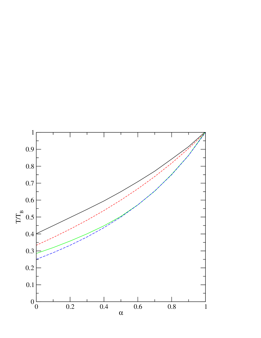
Figure 4: Granular temperatures of the intruder particle normalized by the bath temperature, $T/T_{B}$, versus the coefficient of restitution $\alpha$ when the velocity distribution of the bath is given by Eq. (23) for $M=1$ and $M=0.5$, from top to bottom. Dashed curves correspond to the analytical result MP99 when the velocity distribution of the bath is Gaussian.

Figure 5 displays the intruder particle velocity distribution function for different values of the coefficient of restitution $0.0\leq\alpha\leq 1.0$ when $M=1/2$. The exact solution is known for $\alpha=0.5$, i.e. Eq.(23) with a granular temperature equal to $\alpha$. The simulation results show that in all cases the velocity distribution functions exhibit a power-law tail (See inset of Fig.5) with an exponent independent of $\alpha$ and equal to $-4$.

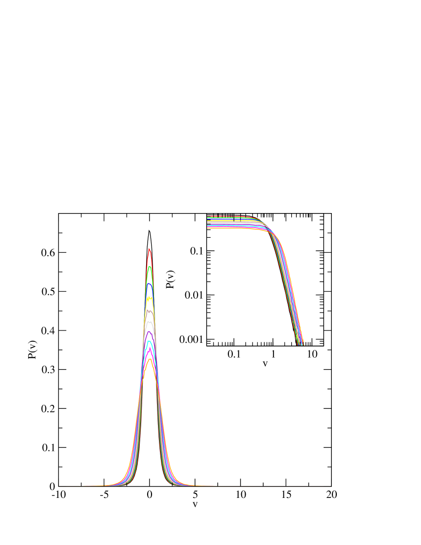
Figure 5: Velocity distribution function of the intruder particle for different values of the coefficient of restitution $\alpha=0.0,0.1,0.2,...0.8,0.9,1.0$, from top to bottom, when $M=1/2$ and when the bath distribution is given by Eq.(23). The insert is a log-log plot showing the algebraic decay of the velocity distribution

3.2 Needle

In this application a needle intruder, confined to a two-dimensional plane, is immersed in a fluid of point particles, each of mass $m$, at a density $\rho$. The needle is characterized by its mass $M$, length $L$ and moment of inertia $I$ and its state is specified by its angular and center of mass velocities, $\omega$ and ${\bf v_{1}}$, respectively (see Fig.6). The velocity distribution of the point particles is again given by Eq 18.

Two main modifications of the Gillespie algorithm are required in order to simulate this system. First, if $v_{1}\neq 0$ the flux is not (on average) constant between collisions. Second, it is necessary to select the point of impact on the needle.

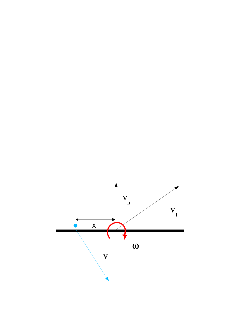
Figure 6: Geometry of the needle-point system

The collision flux on both sides of the needle at a point $-L/2\leq x\leq L/2$ is $\phi({\bf v_{1}}.{\bf n}+\omega x)$. Unlike the case considered above, this flux is time-dependent if $\omega\neq 0$ since the normal vector ${\bf n}$ rotates. Specifically

$$v_{n}={\bf v_{1}}.{\bf n}(t)=v_{1y}\cos(\omega t+\theta_{0})-v_{1x}\sin(\omega t+\theta_{0}),$$ (24)

where $\theta_{0}$ is the orientation of the needle at $t=0$. The total flux over the entire length of the needle is

$$\Phi(t)=\int_{-L/2}^{L/2}\phi({\bf v_{1}}.{\bf n}(t)+\omega x)dx.$$ (25)

For the sake of simplicity we take $a=1$ and $L=1$ and we obtain

$$\Phi(t) = \rho\left(\frac{v_{n}^{2}}{2\omega}+\frac{\omega}{8}+\frac{v_{n}}{2}+\frac{1}{4\omega}\right)erf\left(v_{n}+\frac{\omega}{2}\right)$$ (26)

$$+ \rho\left(\frac{v_{n}^{2}}{2\omega}+\frac{\omega}{8}-\frac{v_{n}}{2}+\frac{1}{4\omega}\right)erf\left(-v_{n}+\frac{\omega}{2}\right)$$

$$+ \rho\frac{e^{-v_{n}^{2}-\frac{\omega^{2}}{4}}}{4\sqrt{\pi}}\left[e^{v_{n}\omega}\left(1-\frac{2v_{n}}{\omega}\right)+e^{-v_{n}\omega}\left(1+\frac{2v_{n}}{\omega}\right)\right].$$

A collision time is generated by solving the equation

$$\int_{0}^{t}dt^{\prime}\Phi(t^{\prime})=-\ln(\xi_{3})$$ (27)

Since the integral cannot be performed analytically, we use the Newton-Raphson method:

$$t_{1}=t-\frac{\int_{0}^{t}\Phi(t^{\prime})dt^{\prime}+\ln(\xi_{3})}{\Phi(t)}$$ (28)

with an initial guess $t=-\frac{\ln(\xi_{3})}{\Phi(0)}$. The procedure is iterative, i.e. $t$ is substituted by $t_{1}$ in Eq.(28), etc. until $|\int_{0}^{t_{1}}\Phi(t^{\prime})dt^{\prime}+\ln(\xi_{3})|$ is smaller than the required precision. In general the convergence is fast and only a few iterations are required. Occasionally, when $\Phi$ is small, the Newton-Raphson method oscillates between two “stable” positions and there is no convergence. When this situation arises, we switch to a bisection procedure. With this modification, the method seems to be robust.

Once the time to collision has been selected, one updates the normal velocity of the center-of-mass of the needle using Eq 24.

In order to choose the position of the impact, one has to calculate the probability that the collision occurs at a distance $x$ from the center of mass of the needle, whatever the velocities of the bath particles, at a given time $t$

$$p(x|t)=\frac{\Phi(v_{n}+x\omega)}{\Phi(v_{n},\omega)},\;\;-1/2\leq x\leq 1/2$$ (29)

This probability is clearly not uniform over the length of the needle. But since it is concave, the maximum is obtained for $x=1/2$ or $x=-1/2$ (if $v_{n}=0$ the probability is a maximum at both ends). We select $x$ using a standard acceptance-rejection method.

Once the position of the impact has been decided, one has to choose if the bath particle collides on the right or left hand side of the needle. The probability of the former event is

$$p(+|x,t)=\frac{\Phi_{+}(v_{n}+x\omega)}{\Phi(v_{n}+x\omega)}$$ (30)

One chooses a random number between $0$ and $1$. If $\xi<p(+|x,t)$, the particle collides with a particle from the right, otherwise the collision is on the left.

Next the velocity of the colliding bath particle must be selected. The probability that the colliding particle has a velocity between $v$ and $v+dv$ is $g_{\pm}(v,v_{n}+x\omega)dv$. It is even more important to sample this distribution carefully than in the one-dimensional case as more extreme velocities are encountered in this system.

Finally, the needle velocity and angular velocity are updated using

$${\bf v_{1}}^{\prime} = {\bf v_{1}}+{\bf n}\frac{\Delta p}{M}$$ (31)

$$I\omega^{\prime} = I\omega+x\Delta p$$ (32)

where

$$\Delta p=-\frac{(1+\alpha){\bf g}.{\bf n}}{\frac{1}{m}+\frac{1}{M}+\frac{x^{2}}{I}},$$ (33)

${\bf n}$ is a unit vector normal to the length of the needle and ${\bf g}={\bf v_{1}}-{\bf v}+\omega x{\bf n}$ is the relative velocity at the point of impact (the velocity of the colliding bath particle also changes, but we do not need to know the new value).

It is necessary to simulate a few hundred thousand to several million collisions in order to obtain good estimates for the properties of interest. The convergence of the simulation is slower when the mass of the needle is much bigger than the bath particle mass.

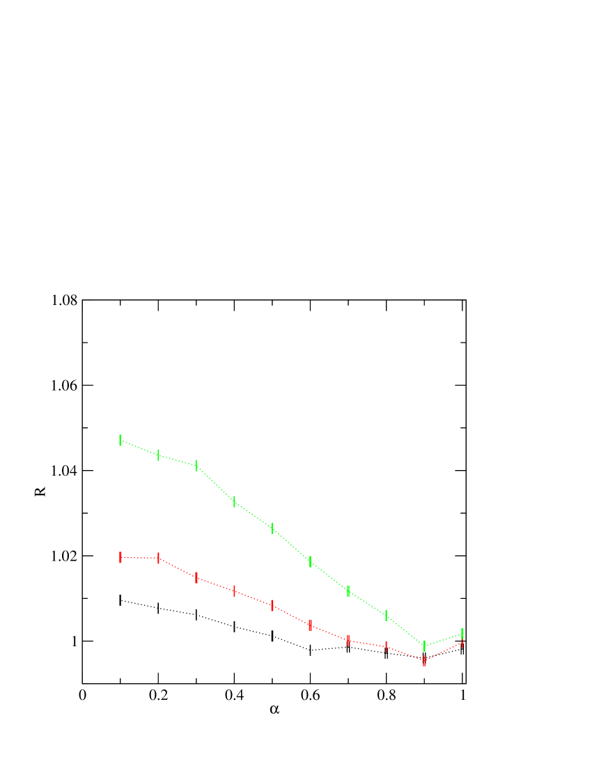
Figure 7: Correlation coefficient, Eq 34, as a function of the coefficient of restitution for $M=0.1,0.5,1$, top-to-bottom

We have previously used this algorithm to confirm a kinetic theory prediction that, when the coefficient of restitution is smaller than unity, the temperature of the bath is larger than the translational granular temperature which is in turn larger than the rotational granular temperature VT04 .

Here we present new results for the cross-correlation between the two degrees of freedom of the needle as a function of the coefficient of restitution, $\alpha$, and for different values of the mass ratio $M/m$. Specifically, we have calculated

$$R=\frac{<v^{2}\omega^{2}>}{<v^{2}><\omega^{2}>},$$ (34)

which is equal to one in equilibrium systems and obviously independent of the mass ratio. Conversely, one observes that for small mass ratios in an inelastic system, there is a positive correlation that increases with decreasing $\alpha$: See Figure 7. We expect this to be a generic feature of anisotropic granular particles in any dimension, regardless of the bath particle velocity distribution.

Unlike the one-dimensional model, where the velocity distribution of the intruder particle is Gaussian for all values of the coefficient of restitution, the translational and angular velocity distributions of the granular needle are never strictly Gaussian (except for elastic collisions). For a large range of values of $M/m$ and $\alpha$, however, the Gaussian is a very accurate approximation. It is only for a light needle and highly inelastic collisions that deviations start to become apparent: See Figure 8.

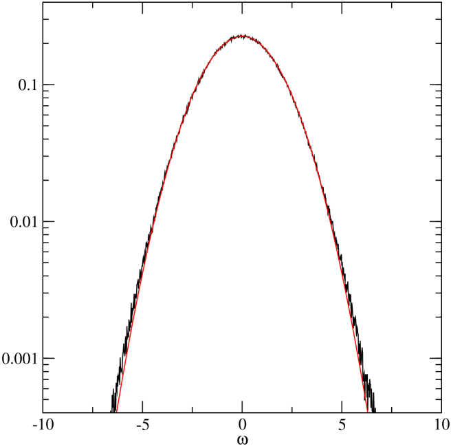
Figure 8: Angular velocity distribution for $M/m=0.1$ and $\alpha=0.1$. Black line: simulation with 5000000 collisions; Red line: best-fit Gaussian

4 DMSC versus Gillepsie algorithm

The two simulation methods provide an exact numerical solution of a Boltzmann equation (they can also be used for inelastic Maxwell modelsBK03 ; BM05 ; BMM05 ). The DSMC algorithm has been described in several articles B94 ; MS00 . For convenience we describe here the version that would be applied to the one-dimensional system discussed in section 3.1.

Velocities sampled from a Gaussian distribution, Eq 18, are assigned to $n_{\rm bath}$ bath particles. A side of the intruder particle is then selected at random: $\sigma_{i1}=+1$ for a collision on the left, $\sigma_{i1}=-1$ for a collision on the right. A bath particle, $i$, is then selected randomly. The collision is accepted with probability $\Theta(v_{i1}\sigma_{i1})\omega_{i1}/\omega_{max}$ where $\Theta(x)$ is the Heaviside function, $\omega_{i1}=2\rho|v_{i1}|$ and $\omega_{max}$ is an upper bound estimate of the probability that a particle collides per unit time. If the collision is accepted a post-collisional velocity, computed from Eq 21, is assigned to the intruder particle. If $\omega_{i1}>\omega_{max}$ the estimate of the latter is updated: $\omega_{max}\leftarrow\omega_{i1}$.

We have implemented this algorithm for the one-dimensional intruder described in section 3.1. We obtain the same results with comparable computational effort.

5 Conclusion

We have shown how the Gillespie algorithm can be used to obtain an exact numerical solution of the Boltzmann equation of an intruder particle in a bath of particles with an arbitrary velocity distribution. We used the method to obtain new results for a one-dimensional system consisting of an intruder particle in a bath with a power law distribution. We also used it to demonstrate, for the first time, the presence of correlations between the translational and rotational momenta of an anisotropic particle.

Although the results presented here apply to the steady state, the method is equally valid for the transient case. It is clear that the Gillespie algorithm offers no significant computational advantage over the DSMC method for these intruder particle systems. It is of interest, however, that two apparently dissimilar methods can be applied to the same physical system. Finally, we note that, as with DSMC, the Gillespie method can be easily generalized to three-dimensional systems.

REFERENCES

REFERENCES

- [1] Pöschel T and Luding S, eds 2001 Granular Gases (Berlin: Springer)
- [2] Pöschel T and Brilliantov N 2003 Granular Gas Dynamics (Berlin: Springer)
- [3] Piasecki J, Talbot J and Viot P 2006 Physica A In press
- [4] Bird G 1994 Molecular gas dynamics and the direct simulation of gas flows (Clarendon Press, Oxford)
- [5] Gillespie D T 1976 J. Comput. Phys. 22 403–434
- [6] Gillespie D T 1977 J. Phys. Chem. 81 2340–2361
- [7] Dufty J W and Brey J J 2005 New Journal of Physics 7 20
- [8] Brey J J, Ruiz-Montero M J and Moreno F 2005 Phys. Rev. Lett. 95 098001
- [9] Martin P A and Piasecki J 1999 Europhys. Lett 46 613
- [10] Viot P and Talbot J 2004 Phys. Rev. E 69 051106
- [11] Gomart H, Talbot J and Viot P 2005 Phys. Rev. E 71 051306
- [12] Puglisi A, Visco P, Trizac E and van Wijland F 2006 Phys. Rev. E 73 021301
- [13] Feitosa K and Menon N 2002 Phys. Rev. Lett. 88 198301
- [14] Wildman R D and Parker D J 2002 Phys. Rev. Lett. 88 064301
- [15] Ben-Naim E, Machta B and Machta J 2005 Phys. Rev. E 72 021302
- [16] Ben-Naim E and Machta J 2005 Phys. Rev. Lett. 94 138001
- [17] Ben-Naim E and Krapivsky P 2003 Granular Gas Dynamics (Berlin: Springer) p 64
- [18] Montanero J M and Santos A 2000 Granular Matter 2 53